- Research Article
- Open access
- Published:
Iterative Fusion of Distributed Decisions over the Gaussian Multiple-Access Channel Using Concatenated BCH-LDGM Codes
EURASIP Journal on Wireless Communications and Networking volume 2011, Article number: 825327 (2011)
Abstract
This paper focuses on the data fusion scenario where  nodes sense and transmit the data generated by a source
  to a common destination, which estimates the original information from
  more accurately than in the case of a single sensor. This work joins the upsurge of research interest in this topic by addressing the setup where the sensed information is transmitted over a Gaussian Multiple-Access Channel (MAC). We use Low Density Generator Matrix (LDGM) codes in order to keep the correlation between the transmitted codewords, which leads to an improved received Signal-to-Noise Ratio (SNR) thanks to the constructive signal addition at the receiver front-end. At reception, we propose a joint decoder and estimator that exchanges soft information between the
  LDGM decoders and a data fusion stage. An error-correcting Bose, Ray-Chaudhuri, Hocquenghem (BCH) code is further applied suppress the error floor derived from the ambiguity of the MAC channel when dealing with correlated sources. Simulation results are presented for several values of
  and diverse LDGM and BCH codes, based on which we conclude that the proposed scheme outperforms significantly (by up to 6.3 dB) the suboptimum limit assuming separation between Slepian-Wolf source coding and capacity-achieving channel coding.
1. Introduction
During the last years, the scientific community has experienced an ever-growing research interest in Sensor Networks (SN) as means to efficiently monitor physical or environmental conditions without necessitating expensive deployment and/or operational costs. Generally speaking, these communication networks consist of a large number of nodes deployed over a certain geographical area and with a high degree of autonomy. Such an increased autonomy is usually attained by means of advanced battery designs, an efficient exploitation of the available radio resources, and/or cooperative communication schemes and protocols. In fact, cooperation between nearby sensors permits the network to operate as a global entity and execute actions in a computationally cheap albeit reliable fashion. Unfortunately, the capacity of SNs to achieve a high energy efficiency is highly determined by the scalability of these sensor meshes. In this context, a large number of challenging paradigms have been tackled with the aim of minimizing the power consumption and improving the battery lifetime of densely populated networks. As such, it is worth to mention distributed compression [1, 2], transmission and/or cluster scheduling [3, 4], data aggregation [5–7], multihop cooperative processing [8, 9], in-network data storage [10], and power harvesting [11, 12]. This work gravitates on one of such paradigms: the centralized data fusion scenario (see Figure 1), where  nodes monitor a given information source
  (representing, for instance, temperature, pressure, or any other physical phenomena) and transmit their sensed data to a common receiver. This receiver will combine the data from the sensors so as to obtain a reliable estimation of the information from the original source
  . When the monitoring procedure at each node is subject to a non-zero probability of sensing error, intuitively one can infer that the more sensors added to this setup, the higher the accuracy of the estimation will be with respect to the case of a single sensor. Therefore, the challenging paradigm in this specific scenario lies on how to optimally fuse the information from all sources while taking into account the aforementioned probability of sensing error, specially when dealing with practical communication channels.

Generic data fusion scenario where  nodes sense a certain physical parameter
  , and transmit the sensed information to a joint receiver.
One of the first contributions in this area was done by Lauer et al. in [13], who extended classical results from decision theory to the case of distributed correlated signals. Subsequently, Ekchian and Tenney [14] formulated the distributed detection problem for several network topologies. Later, in [15] Chair and Varshney derived an optimum data fusion rule which combines individually performed decisions on the data sensed at every sensor. This data fusion rule was shown to minimize the end-to-end probability of error of the overall system. More recently, several contributions have tackled the data fusion problem in diverse uncoded communication scenarios, for example, multihop networks subject to fading [16–18] and delays [19], parallel channels subject to fading [20–22], and asynchronous multiple-access channels [23, 24], among others.
On the other hand, when dealing with coded scenarios over noisy channels, it is important to point out that the data fusion problem can be regarded as a particular case of the so-called distributed joint source-channel coding of correlated sources, since the nonzero probability of sensing error imposes a spatial correlation among the data registered by the sensors. In the last decade, intense research effort has been conducted towards the design of practical iteratively-decodable (i.e., Turbo-like) joint source-channel coding schemes for the transmission of spatially and temporally correlated sources over diverse communication channels, for example, see [25–31] and references therein. However, these contributions address the reliable transmission of the information generated by a set of correlated sensors, whereas the encoded data fusion paradigm focuses on the reliable communication of an information source  read by a set of
  sensors subject to a nonzero probability of sensing error; based on this, a certain error tolerance can be permitted when detecting the data registered by a given sensor. In this encoded data fusion setup, different Turbo-like codes have been proposed for iterative decoding and data fusion of multiple-sensor scenarios for the simplistic case of parallel AWGN channels, for example, Low Density Generator Matrix (LDGM) [32], Irregular Repeat-Accumulate (IRA) [33], and concatenated Zigzag [34] codes. In such references, it was shown that an iterative joint decoding and data fusion strategy performs better than a sequential scheme where decoding and data fusion are separately executed.
Following this research trend, this paper considers the data fusion scenario where the data sensed by  nodes is transmitted to a common receiver over a Gaussian Multiple-Access Channel (MAC). In this scenario, it is well known that the spatial correlation between the data registered by the sensors should be preserved between the transmitted signals so as to maximize the effective signal-to-noise ratio (SNR) at the receiver. On this purpose, correlation-preserving LDGM codes have been extensively studied for the problem of joint source-channel coding of correlated sensors over the MAC [35–38]. In these references, it was shown that concatenated LDGM schemes permit to drastically reduce the error floor inherent to LDGM codes. Inspired by this previous work, in this paper we take a step further by analyzing the performance of concatenated BCH-LDGM codes for encoded data fusion over the Gaussian MAC. Specifically, our contribution is twofold: on one hand, we design an iterative receiver that jointly performs LDGM decoding and data fusion based on factor graphs and the Sum Product Algorithm. On the other hand, we show that for the particular data fusion scenario under consideration, the error statistics in the decoded information from the sensors allow for the concatenation of BCH codes [39, 40] in order to decrease the aforementioned intrinsic error floor of single LDGM codes. Extensive Monte Carlo simulations will verify that the proposed concatenated BCH-LDGM codes not only outperform vastly the suboptimum limit assuming separation between distributed source and channel coding, but also reaches the theoretical residual error bound derived by assuming errorless detection and decoding of the sensor data.
The rest of the paper is organized as follows: Section 2 delves into the system model of the considered encoded data fusion scenario, whereas Section 3 elaborates on the design of the iterative decoding and data fusion procedure. Next, Section 4 discusses Monte Carlo simulation results and finally, Section 5 ends the paper by drawing some concluding remarks.
2. System Model
Figure 2 depicts the system model considered in this work. The information corresponding to a source  (e.g., representing a physical parameter such as temperature) is modeled as a sequence of
  i.i.d binary random variables
  , with
  . A set of
  sensors
  registers blocks of length
 (
( ) from
  , subject to a probability of sensing error
  for all
  , with
  . The sensed sequence at each sensor is then encoded through an outer systematic BCH code
  , where
  and
and  denote the output sequence length and error correction capability of the code, respectively (We hereafter adopt this nomenclature, which differs from the standard notation
  , with
  denoting the minimum distance of the BCH code.). The encoded sequence at the output of the BCH encoder is next processed through an inner LDGM code, that is, a linear code with low density generator matrix
  . The parity check matrix of LDGM codes is expressed as
  , where
  denotes the identity matrix, and
  is a
is a  sparse binary matrix. Variable and check degree distributions (In other words, the parity matrix
  of a
of a  LDGM code has exactly
  nonzero entries per row and
  nonzero entries per column.) are denoted as
  ; the overall coding rate is thus given by
  , where
  is the rate of the outer BCH code. Notice that due to the low density nature of LDGM matrices, correlation is preserved not only in the systematic bits but also in the coded bits. Therefore, in order to exploit this correlation, the generator matrices are set exactly the same for all sensors. The output sequence of the concatenated encoder at every sensor,
  , is composed by a first set of
  bits corresponding to the systematic bits
  , followed by a set of
  BCH parity bits
  and a final set of
  LDGM parity bits
  . These encoded sequences are then BPSK (Binary Phase Shift Keying) modulated and transmitted to a common receiver over a Gaussian Multiple-Access Channel.

Block diagram of the considered scenario.
The signal at the receiver is expressed as

where  stands for the BPSK modulation mapping, and
  represents the average energy per channel symbol and sensor. The Gaussian MAC considered in this work assumes
  and
and  , whereas
  are i.i.d. circularly symmetric complex Gaussian random variables with zero mean and variance per dimension
  . Nevertheless, explanations hereafter will make no assumptions on the value of the MAC coefficients. The joint receiver must estimate the original information
  generated by
  as
as  based on the received sequence
  . This will be done by applying the message-passing Sum-Product Algorithm (SPA, see [41] and references therein) over the whole factor graph describing the statistical dependence between
  and
and  , as will be explained in next section.
3. Iterative Joint Decoding and Data Fusion
In order to estimate the aforementioned original information sequence  , the optimum joint receiver would symbolwise apply the Maximum A Posteriori (MAP) decision criterium, that is,

where  denotes conditional probability. To efficiently perform the above decision criterion, a suboptimum practical scheme would first compute the conditional probabilities of the encoded symbol
  given the received sequence, which is given, for
  and
and  , as
, as

where the proportionality stands for  , and
, and  denotes that all binary variables are included in the sum except
  , that is, the sum is evaluated for all the
  possible combinations of the set
  . Once the
  conditional probabilities for the
  th sensor codeword
  are computed, an estimation
  of the original sensor sequence
  would be obtained by performing (1) iterative LDGM decoding based on
  in an independent fashion with respect to the LDGM decoding procedures of the other
  sensors and (2) an outer BCH decoding based on the hard-decoded sequence at the output of the LDGM decoder. Finally, the
  recovered sensor sequences
  (
( ) would be fused to render the estimation
  as
as

that is, by symbolwise majority voting over the estimated  sensor sequences. Notice that this practical scheme performs sequentially channel detection, LDGM decoding, BCH decoding, and fusion of the decoded data.
However, the performance of the above separate approach can be easily outperformed if one notices that, since we assume  (see Section 2), the sensor sequences
  are symbolwise spatially correlated, that is

for  . As widely evidenced in the literature related to the transmission of correlated information sources (see references in Section 1), this correlation should be exploited at the receiver in order to enhance the reliability of the fused sequence
  . In other words, the considered scenario should take advantage of this correlation, not only by means of an enhanced effective SNR at the receiver thanks to the correlation-preserving properties of LDGM codes, but also through the exploitation of the statistical relation between sequences
  corresponding to different sensors
  . The latter dependence between
  and
and  can be efficiently capitalized by (1) describing the joint probability distribution of all the variables involved in the system by means of factor graphs and (2) marginalizing for
  via the message-passing Sum-Product Algorithm (SPA). This methodology allows decreasing the computational complexity with respect to a direct marginalization based on exhaustive evaluation of the entire joint probability distribution. Particularly, the statistical relation between sensor sequences is exploited in one of the compounding factor subgraphs of the receiver, as will be later detailed.
This factor graph is exemplified in Figure 3(a), where the graph structure of the joint detector, decoder, and data fusion scheme is depicted for  sensors. As shown in this plot, this graph is built by interconnecting different subgraphs: the graph modeling the statistical dependence between
  and
and  for all
  (labeled as SENSING), the factor graph that relates sensor sequence
  to codeword
  through the LDGM parity check matrix
  and the BCH code (to be later detailed), and the relationship between the received sequence
  and the
  codewords
  , with
  (labeled as MAC). Observe that the interconnection between subgraphs is done via variable nodes corresponding to
  and
and  . In this context, since the concatenation of the LDGM and BCH code is systematic, variable nodes
  and
and  collapse into a single node
  , which has not been shown in the plots for the sake of clarity. Before delving into each subgraph, it is also important to note that this interconnected set of subgraphs embodies an overall cyclic factor graph over which the SPA algorithm iterates—for a fixed number of iterations
  —in the order MAC
 LDGM
LDGM BCH
BCH LDGM
LDGM LDGM
LDGM BCH
BCH SENSING.

(a) Block diagram of the overall factor graph corresponding to the proposed iterative receiver; (b) MAC factor subgraph; (c) adaptive flipping of the exchanged soft information between the LDGM and SENSING subgraphs based on the output of the BCH decoder; (d) SENSING factor subgraph.
Let us start by analyzing the MAC subgraph, which is represented in Figure 3(b). Variable nodes  are linked to the received symbol
  through the auxiliary variable node
  , which stands for the noiseless version of the MAC output
  as defined in expression (1). If we denote as
  the set of
  possible values of
  determined by the
  possible combinations of
  and the MAC coefficients
  , then the message
  corresponding to
  will be given by the conditional probability distribution of the AWGN channel, that is

where the value of the constant  is selected so as to satisfy
  . On the other hand, the function associated to the check node connecting
  to
to  is an indicator function defined as

In regard to Figure 3(b), observe that a set of switches controlled by binary variables  and
and  drive the connection/disconnection of systematic (
 ) and parity (
 ) variable nodes from the MAC subgraph. The reason being that, as later detailed in Section 4, the degradation of the iterative SPA due to short-length cycles in the underlying factor graph can be minimized by properly setting these switches.
The analysis follows by considering Figure 3(c), where the block integrating the BCH decoder is depicted in detail. At this point it is worth mentioning that the rationale behind concatenating the BCH code with the LDGM code lies on the statistics of the errors per simulated block, as the simulation results in Section 4 will clearly show. Based on these statistics, it is concluded that such an error floor is due to most of the simulated blocks having a low number of symbols in error, rather than few blocks with errors in most of their constituent symbols. Consequently, a BCH code capable of correcting up to  errors can be applied to detect and correct such few errors per block at a small loss in performance. Having said this, the integration of the BCH decoder in the proposed iterative receiver requires some preliminary definitions.
-
(i)
 : a posteriori soft information for the value
  of the node
  , which is computed, at iteration
  and
and  , as the product of the a posteriori soft information rendered by the SPA when applied to MAC and LDGM subgraphs.
 -
(ii)
 : similar to the previously defined
  , this notation refers to the a posteriori information for the value
  of node
  , which is calculated, at iteration
  and
and 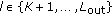 , as the product of the corresponding a posteriori information produced at both MAC and LDGM subgraphs.
 -
(iii)
 : extrinsic soft information for
  built upon the information provided by the rest of sensors at iteration
  and time tick
  .
. -
(iv)
 : refined a posteriori soft information of node
  for the value
  , which is produced as a consequence of the processing stage in Figure 3(c).
 : a posteriori soft information for the value
  of the node
  , which is computed, at iteration
  and
and  , as the product of the a posteriori soft information rendered by the SPA when applied to MAC and LDGM subgraphs.
 : similar to the previously defined
  , this notation refers to the a posteriori information for the value
  of node
  , which is calculated, at iteration
  and
and  , as the product of the corresponding a posteriori information produced at both MAC and LDGM subgraphs.
 : extrinsic soft information for
  built upon the information provided by the rest of sensors at iteration
  and time tick
  .
. : refined a posteriori soft information of node
  for the value
  , which is produced as a consequence of the processing stage in Figure
 Under the above definitions, the processing scheme depicted in Figure 3(c) aims at refining the input soft information coming from the MAC and LDGM subgraphs by first performing a hard decision (HD) on the BCH encoded sequence based on  ,
,  , and the information output from the SENSING subgraph in the previous iteration, that is,
  . This is done
  within the current iteration
  . Once the binary estimated sequence
  corresponding to the BCH encoded block at the
  th sensor is obtained and decoded, the binary output
  is utilized for adaptively refining the a posteriori soft information
  as
as  under the flipping rule

which is performed for  . It is interesting to observe that in this expression, all those indices in error detected by the BCH decoder will consequently drive a flip in the soft information fed to the SENSING subgraph.
Finally we consider Figure 3(c) corresponding to the SENSING subgraph, where the refined soft information from all sensors is fused to provide an estimation of  as
as  . Let
. Let  denote the soft information on
  (for the value
  and computed for
  ) contributed by sensor
  at iteration
  . The SPA applied to this subgraph renders (see [41, equations (5) and (6)])

where  denotes the sensing error probability which in turn establishes the amount of correlation between sensors. Factors
  account for the normalization of each pair of messages, that is,
  for all
  . The estimation
  of
of  at iteration
  is then given by

that is, by the product of all messages arriving to variable node  at iteration
  . The iteration ends by computing the soft information fed back from the SENSING subgraph directly to the corresponding LDGM decoder, namely,

where as before,  represents a normalization factor for each message pair.
4. Simulation Results
To verify the performance of the proposed system, extensive Monte Carlo simulations have been performed for  sensors and a sensing error probability set, without loss of generality, to
  for all sensors. The experiments have been divided in two different sets so as to shed light on the aforementioned statistics of the number of errors per iterations. Accordingly, the first set does not consider any outer BCH coding, and only identical LDGM codes of rate
  (input symbols per coded symbol), variable and check degree distributions
  , and input blocklength
  are utilized at every sensor. The number of iterations for the proposed iterative receiver has been set equal to
  . The metric adopted for the performance evaluation is the End-to-End Bit Error Rate (BER) between
  and
and  , which is averaged over 2000 different information sequences per simulated point and plotted versus the
  ratio per sensor (energy per bit to noise power spectral density ratio). Gaussian MAC is considered in all simulations by imposing
  .
.
Before presenting the obtained simulation results, two different performance limits can be derived for each simulated case. On one hand, it can be easily shown that the aforementioned BER metric can be lower bounded by the probability of erroneously detecting  provided that all sensor symbols
  are perfectly recovered, which can be computed, for even
  , as
, as

that is, as the probability of having more than  sensors in error. On the other hand, the minimum
  per sensor required for reliable transmission of all sensors can be computed by combining the Slepian-Wolf [42] Theorem for distributed compression of correlated sources and Shannon's Separation Theorem. It can be theoretically proven that this Separation Theorem does not hold for the MAC under consideration. However, this limit may serve as a theoretical reference to compare the obtained performance results. This suboptimum limit
  is computed as

where  and the joint binary entropy of the sensors
  is given by

with  denoting the probability of having a sequence with exactly
  zero symbols. In this first simulation set, no outer BCH code is used, hence
  .
.
Figure 4 summarizes the obtained results for this first set of experiments by plotting End-to-End BER versus the difference between the simulated  and the corresponding
  limit from expression (13). Also are depicted horizontal limits corresponding to the BER lower bound from expression (12). First observe that since the aforementioned difference value is negative, the simulated
  is lower than
  , which verify in practice the suboptimality of the computed separation-based bound. On the other hand, notice that the set of all BER curves for
  coincide with the lower bound in expression (12) (horizontal dashed lines), while the waterfall region of such curves degrades as
  increases. However, for
  , the error floor (due to the MAC ambiguity of the received sequence about which transmitted symbol corresponds to each sender) is higher than the lower BER bound. By increasing
  an error floor diminishes at the cost of degrading the BER waterfall performance.

End-to-End BER versus gap to separation limit  for the Gaussian MAC with (a)
  sensors; (b)
  sensors; (c)
  sensors.
It is also important to remark that the results plotted in Figure 4 have been obtained by setting the variables controlling the switches from Figure 3(b) to  during the first iteration, while for the remaining
  iterations
  (i.e., the MAC subgraph is disconnected and does not participate in the message passing procedure). The rationale behind this setup lies on the length-4 loop connecting variable nodes
  ,
,  (
( ),
),  and
and  for
for  , which degrades significantly the performance of the message-passing SPA. Further simulations have been carried out to assess this degradation, which are omitted for the sake of clarity in the present discussion. Based on this result, all simulations henceforth will utilize the same switch schedule as the one used for this first set of simulations.
To better understand the error behavior of the proposed scheme in the error floor region, it is useful to analyze the distribution of the number of errors per block at the output of the LDGM decoders. To this end, let  denote the Cumulative Density Function of the number of errors per LDGM-decoded block
  at iteration
  , which can be empirically estimated based on the results obtained for the first set of simulations. This function
  is depicted for
  and
and  (Figure 5(a)) and for
  and
and  (Figure 5(b)). In this plot, such density function is depicted for every simulated
  point and for every compounding LDGM decoder. Observe that in all the considered
  range, the behavior of the CDF function results in being similar to all sensors. Furthermore, when
  increases (i.e., when the system operates in the error floor region), the resulting
  indicates that most of the decoded blocks contain a relatively small amount of errors with respect to the used blocksize
  . This conclusion also holds for either Figure 5(b) and the other cases addressed in the first set of simulations.

Cumulative Density Function  versus number of errors per LDGM-decoded block
  for (a)
  sensors and
  ; (b)
; (b)  sensors and
  .
.
This statistical behavior of the number of errors per decoded block  motivates the inclusion of an outer systematic BCH code whose error correction capability
  is adjusted so as to correct the residual errors obtained in the error floor region. However, note that the application of an outer code involves a penalty in energy. Specifically, the
  ratio is increased by an amount
  dB, where
  decreases as the error capability
  of the BCH code increases. Consequently, a tradeoff between
  and its associated rate loss must be met. In this context, Figures 6 and 7 represent the End-to-End BER versus the gap to the separation limit
  for
for  (Figures 7(a) and 7(b)),
  (Figures 7(a) and 7(b)), and a number of BCH codes with distinct values of the error-correcting parameter
  . Observe that in all cases the error floor has been suppressed by virtue of the error correcting capability of the outer BCH code, and consequently the lower bound for the BER metric in expression (12) is reached. At the same time, due to the relatively small value of
  with respect to
  , the energy increase incurred by concatenating an outer BCH code is less than 0.5 dB. Summarizing, the proposed iterative scheme can be regarded as an efficient and practical approach for encoded data fusion over MAC, which is shown to outperform the suboptimum separation-based limit while reaching, at the same time, the lower bound for the End-to-End BER.

End-to-End BER versus gap to separation limit  for
for  sensors, different BCH codes and (a)
  ; (b)
; (b)  .
.

End-to-End BER versus gap to separation limit  for
for  sensors, different BCH codes and (a)
  ; (b)
; (b)  .
.
5. Concluding Remarks
In this paper, we have investigated the performance of concatenated BCH-LDGM codes for iterative data fusion of distributed decisions over the Gaussian MAC. The use of LDGM codes permits to efficiently exploit the intrinsic spatial correlation between the information registered by the sensors, whereas BCH codes are selected to lower the error floor due to the MAC ambiguity about the transmitted symbols. Specifically, we have designed an iterative receiver comprising channel detection, BCH-LDGM decoding, and data fusion, which have been thoroughly detailed by means of factor graphs and the Sum-Product Algorithm. Furthermore, a specially tailored soft information flipping technique based on the output of the BCH decoding stage has also been included in the proposed iterative receiver. Extensive computer simulations results obtained for varying number of sensors, LDGM, and BCH codes have revealed that (1) our scheme outperforms significantly the suboptimum limit assuming separation between distributed source and capacity-achieving channel coding and (2) the obtained end-to-end error rate performance attains the theoretical lower bound assuming perfect recovery of the sensor sequences.
References
Pradhan SS, Kusuma J, Ramchandran K: Distributed compression in a dense microsensor network. IEEE Signal Processing Magazine 2002, 19(2):51-60. 10.1109/79.985684
Xiong Z, Liveris AD, Cheng S: Distributed source coding for sensor networks. IEEE Signal Processing Magazine 2004, 21(5):80-94. 10.1109/MSP.2004.1328091
Yao Y, Giannakis GB: Energy-efficient scheduling for wireless sensor networks. IEEE Transactions on Communications 2005, 53(8):1333-1342. 10.1109/TCOMM.2005.852834
Sichitiu ML: Cross-layer scheduling for power efficiency in wireless sensor networks. Proceedings of the 23rd Annual Joint Conference of the IEEE Computer and Communications Societies (INFOCOM '04), March 2004 3: 1740-1750.
Krishnamachari B, Estrin D, Wicker S: The impact of data aggregation in wireless sensor networks. Proceedings of the 22nd International Conference on Distributed Computing Systems, 2002 575-578.
Shrivastava N, Buragohain C, Agrawal D, Suri S: Medians and beyond: new aggregation techniques for sensor networks. Proceedings of the 2nd International Conference on Embedded Networked Sensor Systems, November 2004 239-249.
Tang X, Xu J: Optimizing lifetime for continuous data aggregation with precision guarantees in wireless sensor networks. IEEE/ACM Transactions on Networking 2008, 16(4):904-917.
Aksu A, Ercetin O: Multi-hop cooperative transmissions in wireless sensor networks. Proceedings of the 2nd IEEE Workshop on Wireless Mesh Networks (WiMESH '06), September 2006 132-134.
Yuan Y, Chen M, Kwon T: A novel cluster-based cooperative MIMO scheme for multi-hop wireless sensor networks. Eurasip Journal on Wireless Communications and Networking 2006, 2006:-9.
Xu J, Tang X, Lee WC: EASE: an energy-efficient in-network storage scheme for object tracking in sensor networks. Proceedings of the 2nd Annual IEEE Communications Society Conference on Sensor and AdHoc Communications and Networks (SECON '05), September 2005 396-405.
De Mil P, Jooris B, Tytgat L, Catteeuw R, Moerman I, Demeester P, Kamerman A: Design and implementation of a generic energy-harvesting framework applied to the evaluation of a large-scale electronic shelf-labeling wireless sensor network. Eurasip Journal on Wireless Communications and Networking 2010, 2010:-12.
Seah WKG, Zhi AE, Tan HP: Wireless sensor networks powered by ambient energy harvesting (WSN-HEAP)—survey and challenges. Proceedings of the 1st International Conference on Wireless Communication, Vehicular Technology, Information Theory and Aerospace and Electronic Systems Technology, Wireless (VITAE '09), May 2009 1-5.
Lauer G, Sandell NR Jr., et al.: Distributed detection of known signals in correlated noise. Alphatech, Burlington, Mass, USA; 1982.
Ekchian LK, Tenney RR: Detection networks. Proceedings of the 21st IEEE Conference on Decision and Control 686-691.
Chair Z, Varshney PK: Optimal data fusion in multiple sensor detection systems. IEEE Transactions on Aerospace and Electronic Systems 1986, 22(1):98-101.
Chen H, Varshney PK, Chen B: Cooperative relay for decentralized detection. Proceedings of the IEEE International Conference on Acoustics, Speech and Signal Processing (ICASSP '08), April 2008 2293-2296.
Del Ser J, Olabarrieta I, Gil-Lopez S, Crespo PM: On the design of frequency-switching patterns for distributed data fusion over relay networks. Proceedings of the International ITG Workshop on Smart Antennas (WSA '10), February 2010 275-279.
Lin Y, Chen B, Varshney PK: Decision fusion rules in multi-hop wireless sensor networks. IEEE Transactions on Aerospace and Electronic Systems 2005, 41(2):475-488. 10.1109/TAES.2005.1468742
Thomopoulos SCA, Zhang L: Distributed decision fusion in the presence of networking delays and channel errors. Information Sciences 1992, 66(1-2):91-118. 10.1016/0020-0255(92)90089-Q
Chen B, Jiang R, Kasetkasem T, Varshney PK: Fusion of decisions transmitted over fading channels in wireless sensor networks. Proceedings of the Conference Record of the Asilomar Conference on Signals, Systems and Computers, 2002 2: 1184-1188.
Niu R, Chen B, Varshney PK: Decision fusion rules in wireless sensor networks using fading channel statistics. Proceedings of the Conference on Information Sciences and Systems, March 2003
Chen B, Jiang R, Kasetkasem T, Varshney PK: Channel aware decision fusion in wireless sensor networks. IEEE Transactions on Signal Processing 2004, 52(12):3454-3458. 10.1109/TSP.2004.837404
Lin Y, Chen B, Tong L: Distributed detection over multiple access channels. 2007 IEEE International Conference on Acoustics, Speech and Signal Processing (ICASSP '07), April 2007 541-544.
Li W, Dai H: Distributed detection in wireless sensor networks using a multiple access channel. IEEE Transactions on Signal Processing 2007, 55(3):822-833.
Zhao Y, Garcia-Frias J: Turbo compression/joint source-channel coding of correlated binary sources with hidden Markov correlation. Signal Processing 2006, 86(11):3115-3122. 10.1016/j.sigpro.2006.03.011
Kobayashi K, Yamazato T, Okada H, Katayama M: Iterative joint channel-decoding scheme using the correlation of transmitted information sequences. Proceedings of the International Symposium on Information Theory and Its Applications, 2006 808-813.
Garcia-Frias J, Zhao Y: Near-Shannon/Slepian-Wolf performance for unknown correlated sources over AWGN channels. IEEE Transactions on Communications 2005, 53(4):555-559. 10.1109/TCOMM.2005.844959
Zhong W, Garcia-Frias J: LDGM codes for channel coding and joint source-channel coding of correlated sources. Eurasip Journal on Applied Signal Processing 2005, 2005(6):942-953. 10.1155/ASP.2005.942
Del Ser J, Crespo PM, Galdos O: Asymmetric joint source-channel coding for correlated sources with blind HMM estimation at the receiver. Eurasip Journal on Wireless Communications and Networking 2005, 2005:-10.
Garcia-Frias J, Villasenor JD: Joint turbo decoding and estimation of hidden Markov sources. IEEE Journal on Selected Areas in Communications 2001, 19(9):1671-1679. 10.1109/49.947032
Garcia-Frias J: Joint source-channel decoding of correlated sources over noisy channels. Proceedings of the Data Compression Conference, March 2001 283-292.
Zhong W, Garcia-Frias J: Combining data fusion with joint source-channel coding of correlated sensors. Proceedings of the IEEE Information Theory Workshop (ITW '04), 2004 315-317.
Zhong W, Garcia-Frias J: Combining data fusion with joint source-channel coding of correlated sensors using IRA codes. Proceedings of the Conference on Information Sciences and Systems, 2005
Del Ser J, Garcia-Frias J, Crespo PM: Iterative concatenated zigzag decoding and blind data fusion of correlated sensors. Proceedings of the International Conference on Ultra Modern Telecommunications and Workshops, October 2009
Garcia-Frias J, Zhao Y, Zhong W: Turbo-like codes for transmission of correlated sources over noisy channels. IEEE Signal Processing Magazine 2007, 24(5):58-66.
Zhao Y, Zhong W, Garcia-Frias J: Transmission of correlated senders over a Rayleigh fading multiple access channel. Signal Processing 2006, 86(11):3150-3159. 10.1016/j.sigpro.2006.03.014
Zhong W, Chai H, Garcia-Frias J: LDGM codes for transmission of correlated senders over MAC. Proceedings of the Allerton Conference on Communication, Control, and Computing, 2005
Zhong W, Garcia-Fria J: Joint source-channel coding of correlated senders over multiple access channels. Proceedings of the Allerton Conference on Communication, Control, and Computing, 2004
Hocquenghem A: Codes correcteurs d'erreurs. Chiffres 1959, 2: 147-156.
Bose RC, Ray-Chaudhuri DK: On a class of error correcting binary group codes. Information and Control 1960, 3: 68-79. 10.1016/S0019-9958(60)90287-4
Kschischang FR, Frey BJ, Loeliger HA: Factor graphs and the sum-product algorithm. IEEE Transactions on Information Theory 2001, 47(2):498-519. 10.1109/18.910572
Slepian D, Wolf JK: Noiseless coding of correlated information sources. IEEE Transactions on Information Theory 1973, 19(4):471-480. 10.1109/TIT.1973.1055037
Acknowledgments
This work was supported in part by the Spanish Ministry of Science and Innovation through the CONSOLIDER-INGENIO (CSD200800010) and the Torres-Quevedo (PTQ-09-01-00740) funding programs and by the Basque Government through the ETORTEK programme (Future Internet EI08-227 project).
Author information
Authors and Affiliations
Corresponding author
Rights and permissions
Open Access This article is distributed under the terms of the Creative Commons Attribution 2.0 International License (https://creativecommons.org/licenses/by/2.0), which permits unrestricted use, distribution, and reproduction in any medium, provided the original work is properly cited.
About this article
Cite this article
Del Ser, J., Manjarres, D., Crespo, P.M. et al. Iterative Fusion of Distributed Decisions over the Gaussian Multiple-Access Channel Using Concatenated BCH-LDGM Codes. J Wireless Com Network 2011, 825327 (2011). https://doi.org/10.1155/2011/825327
Received:
Accepted:
Published:
DOI: https://doi.org/10.1155/2011/825327