- Research
- Open access
- Published:
Modeling and energy consumption evaluation of a stochastic wireless sensor network
EURASIP Journal on Wireless Communications and Networking volume 2012, Article number: 282 (2012)
Abstract
In this article, we consider a stochastic model of wireless sensor networks (WSNs) in which each sensor node randomly and alternatively stays in an active mode or a sleep mode. The active mode consists of two phases, called the full-active phase and the semi-active phase. When a referenced sensor node is in the full-active phase of the active mode, it may sense data packets, transmit the sensed packets, receive packets, and relay the received packets. However, when the phase of the sensor node switches from the full active phase to the semi-active phase, it is only able to transmit/relay data. When the referenced sensor node is in a sleep mode, it does not interact with the external world. In this article, first, we develop a stochastic model for the sensor node of a WSN, and then we derive an explicit expression of the stationary distribution of the number of data packets in the sensor node. Furthermore, we figure out some important performance measures, including the sensor node’s energy consumption for transmission, the energy consumption of the sensor operations, and the average energy consumption of the sensor node in a cycle of active and sleep modes. Also, a numerical analysis is provided to validate the proposed model and the results obtained. The novel aspects of our research are the development of a stochastic model for WSN with active and sleep features and the development of important analytical formulae for evaluating the energy consumption of a WSN. These results are expected to be useful as significant contributions to the fundamental theory of the design of various WSNs with active and sleep mode considerations.
Introduction
Wireless sensor networks (WSNs) are composed of a large number of sensors equipped with limited power and radio communication capabilities. Sensors can be deployed in extremely hostile environments, such as battlefield target areas, earthquake disaster areas, and inaccessible areas inside a chemical plant or a nuclear reactor to measure environmental changes or acquire other needed information. Such sensors are usually battery operated, and it is important that they have an acceptable lifetime to accomplish the intended objectives. Hence, energy consumption is a crucial issue, which means that it is important to optimize (i.e., minimize) power usage [1]. There are two major techniques for maximizing the lifetime of the sensor network, i.e., (1) the use of energy efficient routing and (2) the introduction of sleep/active modes for sensors [2]. A good survey of energy-efficient area monitoring for sensor networks was given in an earlier article [3]. The authors have observed that the best method for conserving energy is to turn off as many sensors as possible, while still keeping the system functioning. Most applications for WSNs involve battery-powered nodes with limited energy, and it may not be convenient to recharge or replace the batteries. When a node exhausts its energy, it can no longer sense or relay data. Thus, most of the current research on sensor networks focuses on protocols with energy-efficient mechanisms [4–6].
Another feature of WSNs is their uncertainty, which cannot be ignored when energy issues are addressed. The major uncertainties of WSNs result primarily from (1) uncertain environmental conditions inside the sensor and (2) uncertain environmental conditions outside the sensor. The former includes the uncertainty of time in each of the power modes, the uncertainty of actual lifetime, the uncertainty of the number of transitions between different power modes, the uncertainty of the sensing process, the uncertainty of the transmitting and receiving processes, and the uncertainty of packet delay. The latter includes the uncertainty of the number of sensors in the area to be covered, the uncertainty of relaying requests from neighboring sensors, the uncertainty of routing to the head or the gateway, the uncertainty of their topologies, and many other related uncertainties. Therefore, the investigation of energy-efficient WSNs and their uncertainties is a crucial issue because it offers promise for future developmental improvements in WSNs. Once a system has been designed, additional energy savings can be achieved by using dynamic power management, which shuts down the sensor node if no events occur. Every component in a node can be in different states, e.g., each sensor can be in active, idle, or sleep mode. Mathematically speaking, each sensor will have a finite number of different statuses and the state space of each status also is different. The sensor node stays in each status for a random time and then transfers into another status where it stays for another random duration. A very special case occurs when each sensor only has two different statuses, e.g., active and sleep, similar as those in [7–9]. The sensor node alternatively stays in active or sleep status for a probability distributed duration. In this article, we are going to start this investigation by concentrating on the development of energy consumption in a stochastic WSN and expect our research to improve existing WSN development significantly in both theory and applications.
The rest of this article is organized as follows. “The model description” section gives the description of the modeling, and “Performance characteristics” section concentrates on the investigation of the major performance characteristics of WSNs. And in another section, numerical analysis is provided, and the conclusions and recommendations for future research are stated in last section.
The model description
We considered a WSN in which each sensor node may alternatively stay in two major modes, i.e., active and sleep modes. The active mode consists of two phases, one of which is called the full-active phase (denoted by phase R) and the other phase is called the semi-active phase (denoted by phase N). Sometimes we refer to the sleep mode as phase S. Figure 1 provides a brief description the transition relationship between these phases. From Figure 1, we know that a sensor can switch from the full-active phase to the sleep mode or to the semi-active phase. It can also change from the semi-active phase to the sleep mode or from the sleep mode to the full-active phase.

Phase transition diagram of a sensor node.
In order to better describe the proposed model, the following assumptions and notations are introduced for the sensor node being investigated in this sensor network.
-
(a)
The duration of a sensor in a sleep mode is distributed exponentially with a mean of 1/β. When a sensor is in the sleep mode, it disconnects from the external world. After the sleep duration, the sensor ends its sleep phase and returns to the full-active phase.
-
(b)
The duration that a sensor spends in the full-active phase is a random time that has an exponential distribution with a mean of 1/α. During this period, the sensor node may:
-
(1)
generate packets according to a Poisson process at a rate of λ;
-
(2)
relay packets coming from other sensors in accordance to a Poisson process at a rate of λ E; and
-
(3)
process (transmit or relay) data packets with random exponential time with a mean of 1/μ.
-
(1)
-
(c)
After the period spent in the full-active phase, the sensor node may change to either the semi-active phase or the sleep mode. The former requires there be at least one dada packet waiting to be processed, and the latter occurs when there are no data packets waiting for processing. In the semi-active phase, the sensor node may only process (transmit or relay) data packets with random exponential time with a mean of 1/μ, and it cannot generate or receive any data that are relayed from other sensors. After processing all data packets in the semi-active phase, the senor node will move to the sleep mode automatically.
-
(d)
Each node has sufficient space, or a buffer with infinite size, to store the data it generated or forwarded from other nodes for relaying purposes.
Power consumption models of the radio in embedded devices must take both transceiver and start-up power consumption into account, and there must be an accurate model of the amplifier. In general, the energy consumed per bit transmitted is given [4, 10] in terms of the energy per bit required by the electronic components of the transmitter (including the cost of startup energy), the electronic components of the receiver, the energy consumption of the transmitting amplifier to send one bit over one unit distance, and the path loss factor. In this article, we consider the energy consumption in terms of number of packets transmitted, the sensor mode status, and the switches from one mode to another. We will use the following notations:
-
e tr : the transmitter power consumption per data packet in phase R of the active mode;
-
e t n : the transmitter power consumption per data packet in phase N of the active mode;
-
e or : the operation power consumption per unit time in phase R of the active mode;
-
e on : the operation power consumption per unit time in phase N of the active mode;
-
e os : the operation power consumption per unit time in the sleep mode;
-
e r n : the power consumption when the sensor switches from phase R of the active mode to phase N of the active mode;
-
e rs : the power consumption when the sensor switches from phase R of the active mode to the sleep mode; and
-
e ns : the power consumption when the sensor switches from phase N of the active mode to the sleep mode; and
-
e sr : the power consumption when the sensor switches from the sleep mode to phase R of the active mode.
Performance characteristics
In this section, we derive the distribution of the number of data packets in the sensor node and then develop the explicit expression of the sensor’s important performance measures, including measures of the sensor’s energy consumption, the energy consumption required for operation when the sensor starts from a different mode, the average energy consumption of a sensor in a cycle of full-active mode, semi-active mode, and sleep mode.
Distribution of the number of data packets in the sensor node
In this subsection, we derive the formula of the steady-state probability of the node when there are i (i ≥ 0) packets (including the one being processed and the others that are waiting) in the sensor node. Here, we denote
-
P(R i ) as the steady-state probability of the node when there are i (i ≥ 0) data packets in the referenced sensor node, which is in phase R of the active mode;
-
P(N i ) as the steady-state probability of the node when there are i data packets in the referenced sensor node, which is in phase N of the active mode; and
-
P(S) as the steady-state probability of the node when the node is in the sleep mode.
Our major contribution to this section is the following explicit result.
Theorem 1: Let , and , then
where
Proof: In order to attain the desired result, we had to introduce three stochastic processes. One is the phase status of the node at time t, named I(t). The space of this process consists of the full-active phase (phase R), the semi-active phase (phase N), and the sleep mode (phase S). The second stochastic process is the number of data packets when the sensor is in the full-active phase of the active mode at time t, called X I (t). The space of this process is from 0 to infinity. The third stochastic process is the number of data packets when the sensor is in the semi-active phase of the active mode at time t, called Y I (t). The space of this process is also from 0 to infinity. Based on the description of the sensor node proposed in the previous section and by noting a similar but different consideration as in our other articles [11, 12], it is fairly simple to show that the joint process forms a multiple-dimensional Markov process with the transition rate diagram shown in Figure 2.

Transition rate diagram of the Markov process for sensor.
In Figure 2, the circle notation with R i inside means that the referenced sensor node is in phase R of the active mode and that there are i data packets in the referenced sensor node; the circle notation with N i inside means that the referenced sensor node is in phase N of the active mode and that there are i data packets in the referenced sensor node; the circle notation with S inside means that the referenced sensor node is in sleep mode. If we denote
then the corresponding transition rate matrix, Q, of the constructed multi-dimensional Markov process , can be given by
Now, if we denote for , for , and for , then by applying the matrix analytical methods in stochastic modeling, such as in [13], we can derive the following result:
where matrix R is the minimal non-negative solution to the matrix-quadratic equations
and π0 is the unique positive solution of the equations
in which e is a two-dimensional column vector with all its components of 1, i.e., .
Furthermore, by using Theorem 6.4.1 in [13] to proceed with solving Equations (4) and (5), we finally obtain that
This theorem can now be verified by substituting the above two results in Equation (6) into Equation (3).
Remark: It is straightforward to verify that and if
Measurement of energy consumption of the sensor node
As long as the formula of the steady-state probability is derived, it is not difficult to find various energy-consumption measures of the sensor node. Here, some results are listed to demonstrate how to utilize this formula to obtain the sensor node’s performance measures.
-
(1)
The average energy consumption when the sensor node is in phase R of the active mode is denoted by E TR . Since the sensor will consume e tr milliwatt (mW) of power for transmitting each data packet in phase R of the active mode, and since the expected number of data packets in phase R is , we will have
(7) -
(2)
The average energy consumption when the sensor node is in phase N of the active mode is denoted by E TN . Since the sensor will consume e tn milliwatt (mW) of power to transmit each data packet in phase N of the active mode, and since the expected number of data packets in this phase is , we will have
(8) -
(3)
The average energy consumed per unit time switching from phase R of the active mode to the sleep mode is denoted by E RS . We know that the sensor switches from phase R to phase S only if there are not any data packets awaiting for processing. Since the sensor consumes e rs milliwatt (mW) of power each time it switches from the phase R to phase S, we have the expression for E RS as
(9) -
(4)
The average energy consumed per unit time switching from the full-active phase to the semi-active phase is denoted by E RN . Since the sensor will consume e rn milliwatt (mW) of power each time the sensor switches from the full active phase of the active mode to the semi-active phase, and since the expected number of switching times from active mode to sleep mode per unit time is , therefore we have
(10) -
(5)
The average energy consumed per unit time switching from the sleep mode to phase R of active mode is denoted by E SR . Since the sensor will consume e sa milliwatt (mW) of power each time the sensor switches from the sleep mode to the full-active mode, and since the expected switching number from the sleep mode to the full-active phase per unit time is P(S) β, we will have
(11)
Node operation metrics
Now, several major metrics of the sensor node’s operation are discussed, including
-
(1)
The average delay of a data packet in the sensor node, denoted by D. Since the sensor’s data generating rate is λ and since the rate of the sensor’s relay requests from other sensors is λ E , by using Little’s law [14], we have
(12) -
(2)
The throughput, denoted by T n , of a sensor node which is defined as the average number of the data packets transmitted from the sensor per unit time, then
(13) -
(3)
The probability that the sensor node is actually in sleep mode and the probability that the sensor node is in the active mode. If we denote P S as the probability that the sensor node is actually in sleep mode, and if we denote P A as the probability that the sensor node is in the active mode, from our Theorem 1, we have
(14)
Remark: Based on the explicit results presented above, it is apparent that the probability that the sensor is in sleep mode is not equal to , and the probability that the sensor in active mode is not equal to , since the sensor node has to relay all data packets in the node when the sensor’s mode switches from phase R to phase N. This means that the active-sleep model we developed is not a standard stochastic renewal process.
Energy consumption for operation
In this section, we concentrate on the sensor’s average energy consumption during operation in the full-active phase, semi-active phase, and sleep mode, which is denoted by E OR , E ON , and E OS , respectively.
Since the sensor node will stay in the sleep mode for an exponentially distributed random time, and since the energy consumption per unit time in sleep mode is e os , it is easy to determine that , where is the average sleep time.
Now, we consider how to obtain the sensor’s energy consumption during its operation in phase N (semi-active phase) and phase R (full-active phase).
-
(1)
The operation energy consumption in the duration starting from the time when there are i data packets in phase N to the time when all data have been processed, denoted by . In this case, the sensor node only can continuously transmit the data packets that are already in the buffer of the sensor, and it cannot sense or receive any other data packets. The operation time in phase N is the summation of the transmission time for all those data packets. If we denote the operation time by T N,i , when starting from the time when there are i data packets in phase N, based on the assumption of the transmission time for each data packet, we know that this time is an i-Erlang random variable and that it possesses the following probability density function:
(15)Therefore, the average energy consumption for the duration of the operation, starting from the time when there are i data packets in the semi-active phase and ending with the time when all data packets have been processed, can be given by
(16)The average energy consumption for the operation of a sensor in the phase N is
(17) -
(2)
The operation energy consumption when starting from the time when there are i data packets in phase R, denoted by E OR,i . Note that, in this case, the sensor node in phase R of active mode can sense, receive, and transmit data packets and switch to phase N or phase R. When the sensor switches its phase from phase R to phase N, the sensor node only can continuously transmit the data packets that were already in the buffer of the sensor, and it cannot sensor or receive any other data packets. Thus, the operation time in this case is not as simple as the T N,i defined in above (1). In order to determine the distribution of this operation time when there are i data packets in phase R of the active mode, we define the state when the sensor node is in sleep status as an absorbing state and construct a new Markov process with the following transition rate diagram with absorbing state (Figure 3). If we denote the operation time by T R,i when starting from the time when there are i data packets in phase R, then, from the definition of the distribution of the phase type as introduced in [15], we know that the distribution function of the actual operation time is a phase-type distribution and has an expression as
(18)for x ≥ 0, where Matrix T can easily be determined from the diagram in Figure 3 as
where , , and . Therefore, the average energy consumption during operation, when starting from the time when there are i data packets in phase R to the time when the node reached a sleep node or phase N, is given by
(19)Figure 3 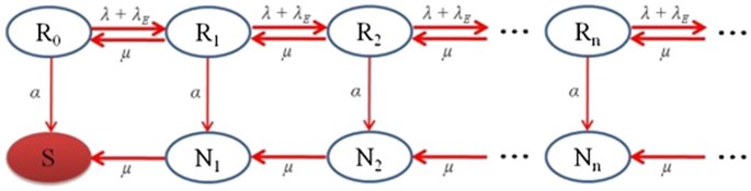
Transition rate diagram of Markov process with absorbing state.
When the node is in phase R and there are i data packets, denote the initial probability by αi, and the probability vector . Then, the energy consumption during operation in phase R, starting from the initial probability α i , can be expressed as
(20)

Total average energy consumption in a cycle of active sleep modes
In this section, we consider the total active average energy consumption in a cycle of active and sleep modes, denoted by Ecycle. Without loss of generalization, we will ignore the switch energy consumption between sensor phases and define the cycle as the time period between the epoch when the sensor just starts its full active phase and the epoch when the sensor ends its sleep mode. In a trivial case when no data are actively processed during the cycle, the total average energy consumption is the summation of energy consumption the sensor needs to operate when there is no any data packet in the sensor and that when the sensor is in sleep, i.e.,
However, in the non-trivial case when at least a data packet is processed during the cycle, the energy consumption in this cycle should include
-
the energy consumption during operation in the sleep mode, E OS ;
-
the energy consumption during operation in phase R of the active mode, E OR ;
-
the energy consumption during operation in phase N of the active mode, E ON ;
-
the energy consumption for transmission in phase R of the active mode, E TR ;
-
the energy consumption for transmission in phase N of the active mode, E TN .
Therefore, based on our results in “Measurement of energy consumption of the sensor node” and “Energy consumption for operation” sections above, we will have
Numerical analysis
To verify the validity of the analytical expressions obtained in the previous section, we present the numerical results for a set of specific parameters in this section. The performance measures considered here are several energy consumptions, data package time delay, and the throughput.
In the model presented in this article, no limit is specified for the sensor’s data storage capacity. However, in [16], we assumed that the data storage capacity of the sensor node was a finite number C. Therefore, as a comparison, in the following figures in this section, we treat the sensor’s data storage capacity in this model as an infinite number, i.e., . In addition, different performance measures for different C values (C = 20, 10, 5) in [16] are also included in all figures. We observed and compared the effects of various performance measures in the four cases, i.e., C = ∞, 20, 10, and 5 versus the sensor node’s generating rate λ. We let λ change from 0.05 to 0.5. As a comparison, we used the same parameters for this article as were used in [16], which are listed in Table 1.
Figure 4 shows the energy consumption when the senor node switches from phase R of the active mode to sleep mode S. It is clear that, with the increase of the sensor’s generating rate λ from 0.05 to 0.5, the switching energy assumption increases slowly. Thus, from the viewpoint of minimizing the energy consumption for switching from active mode to sleep mode, minimizing the number of data packets will not have much effects. It also can be observed that the curve with “C = 20” is much closer to the one with “C = ∞” than the other two curves of “C = 10” and “C = 5”. It is reasonable to expect that the case with larger C value would be closer to the case in which C = ∞.

Energy consumption for switching from the phase R to the sleep mode.
Figure 5 shows the energy consumption when the sensor node switches from sleep mode to the active mode. In this case, the energy consumption does not increase with the sensor’s generating rate, but it decreases slightly. This is because that the increased generating rate may increase the average time that the sensor stays in active mode, reduces the number of sleeps over a unit observation time and therefore reduces the energy consumption of switching from sleep mode to the active mode. In addition, similar to Figure 4, it also can be seen that the curve with “C = 20” is much closer to the one with “C = ∞” than the other two curves of “C = 10” and “C = 5”, which further verifies the validity of our formulae.

Energy consumption for switching from the sleep mode to the phase R.
We also investigated the relationship between the change of the sensor’s generating rate λ and the average energy assumption for transmitting a package in phase R or phase N. The curves in Figures 6 and 7 show that, with the increase of the generating rate λ, these two kinds of energy consumption will increase. This means that transmitting more data packages cause an increase in consumption. As mentioned during the discussion of the design of a WSN, the balance between energy consumption and the generation of packages is a critical issue.

Energy consumption for transmitting in the phase N the active mode.

Energy consumption for transmitting in the phase R of the active mode.
The average data delay is depicted in Figure 8. The curve with “C = ∞” is the delay curve for the model in this article. It is obvious that the data delay increases when either the sensor’s generating rate λ increases or a greater number of relayed messages are being processed. Throughput of the sensor node is shown in Figure 9, and it depicts what we expected in that the throughput increases as the sensor’s generating rate increases.

Average data delay vs. sensor’s generate rate.

Throughput of sensor node vs. sensor’s generate rate.
Conclusions
In this article, we have reported the results of our study of the energy consumption of a WSN. By developing a stochastic model of the sensor node of WSNs and applying the stochastic method, we derived the explicit expression of the distribution of the number of an data packets in a sensor node. Then, we determined several important performance matrices related to the sensor node’s energy consumption. Numerical analysis was provided to validate the proposed model and the results obtained. The results show that the energy consumption for switching between the active mode and sleep mode does not depend significantly on the number of data packets. However, the energy consumption for transmitting the data packets depends on the rate at which data packets are generated, which means that transmitting high-density data requires the expenditure of more energy. The proposed model and analysis method are expected to be applied to the design and analysis of various WSNs, taking the times spent in active and sleep modes into consideration.
References
Maheswar R, Jayaparvathy R: Optimal power control technique for a wireless sensor node: a new approach. Int. J. Comput. Electric. Eng. 2011, 3(1):1793-8163.
Quan Z, Subramanian A, Sayed AH: REACA: an efficient protocol architecture for large scale sensor networks. IEEE Trans. Wirel. Commun. 2007, 6(8):2924-2933.
Carle J, Simplot-Ryl D: Energy-efficient area monitoring for sensor networks. IEEE Comput. Mag. 2004, 37(2):40-46.
Haapola J, Shelby Z, Pomalaza-Raez CA, Mahoen P: Crosslayer energy analysis of multi-hop wireless sensor networks, in Proceedings of the European Workshop on Wireless Sensor Networks. Turkey: Istanbul; 2005.
Jones CE, Sivalingam KM, Agrawal P, Chen JC: A survey of energy efficient network protocols for wireless networks. Wirel. Netw. 2001, 7(4):343-358. 10.1023/A:1016627727877
Shah R, Rabaey J: Energy aware routing for low energy ad hoc sensor networks, in Proceedings of the IEEE Wireless Communications and Networking Conference. FL: Orlando; 2002.
Chiasserini CF, Garetto M: Modeling the performance of wireless sensor networks. Hong Kong, China: Proceedings of IEEE INFOCOM’04; 2004:9-11.
Chiasserini CF, Garetto M: An analytical model for wireless sensor networks with sleeping nodes. IEEE Trans. Mob. Comput. 2006, 5(12):1706-1718.
Hsin CF, Liu M: Randomly duty-cycled wireless sensor networks: dynamics of coverage? IEEE Trans. Wirel. Commun. 2006, 5(11):3182-3192.
Tang S, Li W: QoS supporting and optimal energy allocation for a cluster based wireless sensor network. Comput. Commun. 2006., 29(2569–2577):
Li W, Alfa AS: A PCS network with correlated arrival process and splitted-rate channels. IEEE J. Sel. Areas Commun. 1999, 17(7):1318-1325. 10.1109/49.778188
Li W, Fang Y: Performance evaluation of wireless cellular networks with mixed channel holding times. IEEE Trans. Wirel. Commun. 2008, 7(6):2154-2160.
Latouche G, Ramaswami V: Introduction to Matrix Analytic Methods in Stochastic Modeling, ASA-SIAM Series on Statistics and Applied Probability. Philadelphia: SIAM; 1999.
Harrison PG, Patel NM: Performance Modelling of Communication Networks and Computer Architectures (Addison Wesley. MA: Reading; 1993.
Netuts MF: Matrix-Geometric Solutions in Stochastic Models (The Johns Hopkins University Press. MD: Baltimore; 1981.
Zhang Y, Li W: An energy-based stochastic model for wireless sensor networks. Wirel. Sensor Netw 2011., 3(322–328):
Acknowledgments
This study was supported in part by the NSF under grant CNS-1059116 and HRD-1137732.
Author information
Authors and Affiliations
Corresponding author
Additional information
Competing interests
The authors declare that they have no competing interests.
Authors’ original submitted files for images
Below are the links to the authors’ original submitted files for images.
Rights and permissions
Open Access This article is distributed under the terms of the Creative Commons Attribution 2.0 International License (https://creativecommons.org/licenses/by/2.0), which permits unrestricted use, distribution, and reproduction in any medium, provided the original work is properly cited.
About this article
Cite this article
Zhang, Y., Li, W. Modeling and energy consumption evaluation of a stochastic wireless sensor network. J Wireless Com Network 2012, 282 (2012). https://doi.org/10.1186/1687-1499-2012-282
Received:
Accepted:
Published:
DOI: https://doi.org/10.1186/1687-1499-2012-282