- Research
- Open access
- Published:
Blind recognition of binary cyclic codes
EURASIP Journal on Wireless Communications and Networking volume 2013, Article number: 218 (2013)
Abstract
A solution to blind recognition of binary cyclic codes is proposed in this paper. This problem could be addressed on the context of non-cooperative communications or adaptive coding and modulations. We consider it as a reverse engineering problem of error-correcting coding. The proposed algorithm recovers the encoder parameters of a cyclic, coded communication system with the only knowledge of the noisy information streams. By taking advantages of soft-decision outputs of the channel and by employing statistical signal-processing methods, it achieves higher recognition performances than existing algorithms which are based on algebraic approaches in hard-decision situations. By comprehensive simulations, we show that the probability of false estimation of coding parameters of our proposed algorithm is much lower than the existing algorithms, and falls rapidly when signal-to-noise ratio increases.
1. Introduction
T he blind recognition of cyclic codes is a reverse engineering problem of the error-correcting coding which can be applied to non-cooperative communications [1, 2] and adaptive coding and modulations (ACM) [3–6]. In most cases of digital communications, forward error-correcting coding is used to protect the transmitted information against noisy channels to reduce errors which occur during transmission. Cyclic codes are one class of the most important error-correcting codes applied in communication area. In cooperative context, the parameters of the codes and modulations are usually known by the transmitters and receivers both. But a receiver in non-cooperative communications or a cognitive radio receiver may not know those parameters and thus cannot directly receive and decode the transmitted information on the channel. Therefore, to adapt itself to an unknown transmission context, the receiver must recognize the modulation and coding parameters blindly before processing the received data. In this paper, we develop an approach for blind recognition of the coding parameters of a communication system which uses binary cyclic codes.
2. Related work
In [7], a Euclidean algorithm-based method is proposed to identify a 1/2-rate convolutional encoder in noiseless cases. However, it is not suitable for noisy channels. In [8], another approach is presented to identify a 1/n-rate convolutional encoder in noisy cases based on the Expectation Maximization algorithm. The authors of [9, 10] develop methods for blind recovery of convolutional encoder in turbo code configuration. In [6, 11], a dual code method for blind identification of k/n-rate convolutional codes is proposed for cognitive radio receivers. An iterative decoding-technique-based reconstruction of block code is introduced by the authors of [12] and was applied to low-density parity-check (LDPC) codes. An algebraic approach for the reconstruction of linear and convolutional codes is presented in [13]. In [14], an algorithm for blind recognition of error-correcting codes is presented by utilizing the rank properties of the received stream.
In [15], an approach for blind recognition of binary linear block codes in low code-rate situations is presented. The authors propose to estimate the code length according to the code weight distribution characters of the low-rate codes and then get the generator matrix by improving the traditional simplification of matrices. It has a good performance in high bit error rate (BER) but is not suitable for high code rate situations. Furthermore, it requires a large amount of observed data. In [16] and [17], the authors present a blind recognition algorithm for Bose-Chaudhuri-Hocquenghem (BCH) codes based on the Roots Information Dispersion Entropy and Roots Statistic (RIDERS). This algorithm can achieve correct recognition in both high and low code rate situations with the BER of 10−2. But it is computationally intensive, especially when the code length is large. The authors of [18] improve the algorithm proposed in [16, 17] by reducing the computational complexity and making the recognition procedure faster.
Most of the previous works are concentrating on hard-decision situations, and are based on utilizing the algebraic properties of the codes in Galois fields (GF). The major drawback of them is that they have a low fault tolerance. Even if only 1 bit error occurs in a codeword, the algebraic properties of error-correcting codes will be largely destroyed. Therefore, the recognizers need a large amount of observed data. On the other hand, if soft information about the channel output is available, the soft-decision outputs can provide more information for the code recognition, and statistical signal processing algorithms can also be employed to improve the recognition performance.
When statistic and artificial-intelligence-based iterative algorithms are applied to error-correcting decoding, the decoding performance is improved about 2 ~ 3 dB in soft-decision situations [19]. In [20, 21], the authors introduce a MAP approach to achieve blind frame synchronization of error-correcting codes with a sparse parity-check matrix. It is also developed on Reed Solomon (RS) codes [22] and BCH product codes [23] and yields better performances than previous hard decision ones. In this paper, we propose an algorithm to achieve blind recognition of binary cyclic codes in soft-decision situations. Literature [4] also considers the blind recognition of coding parameters based on soft decisions. But in fact, its recognition procedure is semi-blind. The authors assume that the channel code which is used at the transmitter is unknown to the receiver, but the code is chosen from a set of possible codes which the authors call the candidate set. This set has a limited number of candidates, and is arranged beforehand by both the transmitter and the receiver. It has good performances on ACM, but is not suitable for non-cooperative cases.
To the best of our knowledge, this paper is the first publication to consider the complete-blind recognition problem of binary cyclic codes in soft-decision situations. The proposed algorithm in this paper is based on the RIDERS algorithm introduced in [16–18]. We improve and extend this work in order to handle soft-decision situations. To utilize the soft-decision outputs, we employ the idea of MAP-based processing method proposed in [20–23].
The remainder of this paper is organized as follows: section 3 briefly introduces the RIDERS algorithm in hard decision situations proposed in [16–18]; section 4 presents the principle of our proposed recognition algorithm for binary cyclic codes in soft-decision situation; section 5 draws the general recognition procedure of the proposed algorithm; and finally, the simulation results and conclusions are given in sections 6 and 7.
3. RIDERS algorithm for blind recognition of BCH codes
3.1 Introduction of RIDERS algorithm
The RIDERS algorithm is introduced in [16, 17] and improved in [18] to solve the problem of recognition of BCH codes. The system model of blind recognition problem of coding parameters is shown in Figure 1. On the transmitter, the information sequence T m is encoded and separated to coded blocks T c by the encoder and modulated before transmitted to the channel. After demodulation, the receiver blindly recognizes the coding parameters and decodes the received blocks R c to correct the errors which occur during the transmission. R m is the decoded information which could be processed forward.

The system model of the blind recognition problem of coding parameters.
We define c(x) to be the codeword polynomial of T c , then the algebraic model of the encoding procedure can be described as follows [24]:
or in systemic form:
where m(x) is the input information polynomial and g(x) is the generator polynomial. The purpose of the recognition is to estimate the codeword length and generator polynomial g(x) blindly with the only knowledge of the received streams. For an encoding system, m(x) is different in each codeword, but g(x) is the same. According to Equations 1 and 2, the roots of g(x) are also the roots of c(x). If no error occurs, the roots of g(x) will appear in every codeword. However, for an invalid codeword, this algebraic relationship does not exist. In this paper, we define the code roots as the roots of the generator polynomial. The root space of a binary codeword polynomial c(x) defined in GF(2m) (m ≥ 1) is a finite space, which contains 2m − 1 symbols. We define A to be the set of the generator polynomial roots. In a noisy context, statistically, for each codeword c(x), the probabilities of the codeword polynomial roots appear in A is larger than that in (defined in GF(2m)). While for an invalid codeword polynomial c’(x), the roots of c’(x) appear randomly in GF(2m). In this case, the authors of [16–18] propose the following unproved hypothesis:
Hypothesis 1: Each symbol in GF(2m) has a uniform probability of being a root of c’(x).
According to this hypothesis, the authors of [16–18] propose an algorithm to recognize the BCH code length by traversing all the possible code length and primitive polynomials to find the correct coding parameters that maximize the roots Information Dispersion Entropy Function (IDEF) as follows:
where n = 2m − 1 is the code length, p i (1 ≤ i ≤ 2m − 1) is the probability of αi to be the root of the code and α is a primitive element in GF(2m). p i is calculated as follows:
The received sequence, i.e. R c in Figure 1, is separated to M packets with an assumption of code length l, as shown in Figure 2. In [16–18], the authors assume that the start point of the first coding packet is obtained according to the frame synchronization testing, while the code length and generator polynomial are unknown. We define r j (x)(1 ≤ j ≤ M) to be the codeword polynomial of the j th packet in the received sequence. In Equation 4, N i is the times of appearances of αi being the root of r j (x) in the M packets, and .

The received sequence separated to M packets.
According to Hypothesis 1, when the estimation of code length and primitive polynomial is incorrect, p i could be considered uniformly distributed, and p i ≈ 1/(2m − 1) (1 ≤ i ≤ 2m − 1). Thus the ∆H in Equation 2 is low. If the code parameters are estimated correctly and αi is a root of g(x), p i should be larger. Therefore, the distribution of p i should not be uniform. Then the information entropy of p i is lower and ∆H is larger. This is the basic principle of estimating the code length by maximizing the ∆H defined in Equation 3.
Once the code length is estimated, by comparing p i at different roots, we can consider the obviously higher ones as the estimation of the code roots and the generator polynomial could be obtained by , where are the estimated code roots, i.e. the roots of the generator polynomial.
The RIDERS algorithm has a good performance but there are still some drawbacks which need to be improved, which are described as follows:
-
1)
Hypothesis 1 proposed in [16–18] is not correct. In section 3.2, we give the proof. In fact, not all the symbols in GF(2m) have the same probability of being a root of an invalid codeword c’(x).
-
2)
This algorithm only considers the BCH codes in the cases of regular code length, i.e. code length l = 2m − 1. The authors ignored the shortened code case, which are widely applied, however.
-
3)
The code roots can be separated into some conjugate root groups, and each group contains several conjugate roots, which are the roots of a same minimal polynomial. If a generator polynomial g(x) has a root β, which is a root of the minimal polynomial m p (x), the symbols which are other roots of m p (x) also are part of the roots of g(x). So we can test which minimal polynomials are factors of the generator polynomial rather than testing which elements in GF(2m) are roots of the code.
-
4)
This algorithm is based on the hard decision symbols and do not utilize the soft channel outputs
-
5)
This algorithm only considers the recognition of BCH codes and does not discuss the applications on other binary cyclic codes.
-
6)
The authors of [16–18] ignore the synchronization of the codewords. They assume that the starting positions of the codewords have been known before the recognition procedure by framing testing. But in practical implementations, this should not be the case in blind context.
In the paragraph from section 4, we propose an improved RIDERS algorithm based on soft-decision situations and extend the applications to general binary cyclic codes.
3.2 Proof of faultiness of Hypothesis 1
In this section, we present that Hypothesis 1 proposed in [16–18] is not always correct. The proof is shown below.
Proof. Let c’(x) be the codeword polynomial of a codeword C ’ , we can calculate p i , which is the probability that αi is a root of c’(x). To calculate p i , we define the minimal parity-check matrix Hmin (αi) corresponding to the element αi in GF(2m) as follows:
We transform Hmin (αi) to its binary form by replacing the symbols in Hmin (αi) by their binary column vector patterns according to the coding theory [25] and record it Hbmin (αi).
For example, the minimal parity-check matrix Hmin (α3) corresponding to the element α3 in GF(23) with code length l = 23 − 1 = 7 is as follows:
Based on the primitive polynomial p(x) = x3 + x + 1, we can replace the symbol α3 by the vector [011]T, and other symbols are processed similarly. Then the parity-check matrix can be written in GF(2) as follows:
If αi is a root of c’(x), we have
There are m rows in Hbmin(αi) and we define h μ (1 ≤ μ ≤ m) to be the μ th row of Hbmin(αi). Then the equation Hbmin(αi) × C′ = 0 means that the product of any row of Hbmin(αi) with the codeword C’ equals to zero, as shown in Equation 9:
So we can calculate the probability of αi being a root of c’(x), i.e. the probability of Hbmin(αi) × C′ = 0 as follows:
In the following paragraphs of this paper, we define P r (x) as the probability of x. Let hμ,u(1 ≤ u ≤ n) and C u be the u th elements in the vector h μ and C’ and we define the checking indexing set S μ for h μ and C’ as follows:
Obviously, when the number of nonzero elements in S μ is even, we have
And when the number of nonzero elements in S μ is odd, we have
When C’ is not a valid codeword, i.e. the elements in C’ can be considered to appear randomly, the probabilities of the number of nonzero elements in S μ being odd and even are all about 0.5. When Hbmin(αi) is full rank (the rank is calculated in GF(2)), the rows of Hbmin(αi) is linearly independent, so we can calculate Equation 10 as follows:
But if Hbmin(αi) is not full rank, the calculation of P r [Hbmin(αi) × C = 0] by Equation 14 is not correct. We define the maximum linearly independent vector group MI of the row vectors set H = {h μ |1 ≤ μ ≤ m} as follows:
MI is a subset of H and meets the following conditions:
-
(1)
The vectors in MI are linearly independent;
-
(2)
Any vector in H can be obtained by linear combinations of the vectors in MI.
And it is easy to prove that the number of vectors in MI equals to the rank of Hbmin(αi).
According to the condition 2 of the definition of MI, if all the vectors in {h μ |h μ ∈ MI} make h μ × C = 0, then also for all the vectors in {h μ |h μ ∈ H}, we have h μ × C = 0. So the calculation of Equation 10 should be:
where the elements in are the vectors in MI, i.e. a maximum linearly independent vector group of the rows of Hbmin(αi).
According to Equation 15, Hypothesis 1 is true only if all the Hbmin(αi), where 1 ≤ i ≤ 2m − 1, have the same rank. Unfortunately, this condition cannot always be met. For example, we have the following results over GF(26):
Therefore, we have
Therefore, we can get the conclusion that Hypothesis 1 proposed in [16–18] is not correct.
Figure 3 shows the probabilities that the elements in GF(26) are the roots of a random block with length l = 63 by simulations.

Probability of the elements in GF(2 6 ) being the roots of random codes.
4. Blind recognition algorithm in soft-decision situations
4.1 Code length estimation and blind block synchronization
Soft outputs of the channel could provide more information about the reliability of each decision symbol. In this section, we propose an approach to improve the recognition performance by employing the soft decisions.
We define c r (x) to be the codeword polynomial of a code block C r . According to the algebraic principles of cyclic codes, if αi is a root of c r (x), we have c r (αi) = 0 and Hmin(αi) × C r = 0. In soft-decision situations, instead of verifying whether αi is a root of each block, we can calculate p j,i , the probability that αi is a root of the j th block in the received sequence as shown in Figure 2, and calculate p i in Equation 4 as follows:
where M is the number of blocks, as shown in Figure 2.
The elements in an extension field GF(2m) can be separated to some groups according to the minimal elements over GF(2m). Each minimal polynomial has several roots in GF(2m), we call the set of them as a conjugate element group in this paper. And the generator polynomial of a cyclic code can be factorized by some minimal polynomials as follows:
Because the generator polynomial g(x) is a factor of a valid codeword polynomial c(x), the minimal polynomials in Equation 19 are also the factors of c(x). So if an element αi(1 ≤ i ≤ 2m − 1) in GF(2m) is a root of c(x), the elements which have the same minimal polynomial with αi are also the roots of c(x). Therefore, we can just calculate p′ λ (1 ≤ λ ≤ q), the probability that the minimal polynomial m λ (x)(1 ≤ λ ≤ q) is a factor of c r (x), where q denotes the number of minimal polynomials over GF(2m). According to this idea, we can modify Equation 18 to Equation 20 to calculate p′ λ rather than p i . This modification can reduce the calculation complexity because the number of minimal polynomials over GF(2m) is severely lower than the number of elements in GF(2m). In Equation 20, p′ j,λ denotes the probability that m λ (x) is a factor of the codeword polynomial of the j th block in the observed window as shown in Figure 2.
And the IDEF defined in Equation 3 should be modified to Equation 21:
To calculate p′ j,λ in Equation 20, which is the probability that a minimal polynomial m λ (x) is a factor of c r (x), we can define the binary minimal parity-check matrix Hbmin(m λ (x)) corresponding to m λ (x) and calculate the probability of Hbmin(m λ (x)) × C r = 0.
The coefficients of m λ (x) are in GF(2) and m λ (x) can be written as follows:
where e is the degree of m λ (x). g e , ge − 1, ⋯, g1 and g0 are all in GF(2). According to these coefficients of m λ (x), we can obtain the minimal polynomial-based binary, minimal parity-check matrix Hbmin(m λ (x)) with the following steps.
-
1)
We assume the code length is l and initialize a matrix G as follows:
In Equation 23, the number of rows and columns are l-e and l, respectively.
(23) -
2)
Transform the left e × e area of G to an identity matrix I by elementary row transformation as follows:
where Q is a matrix, which has l-e rows and e columns.
(24) -
3)
The minimal parity-check matrix can be obtained as follows:
(25)
According to the algebraic principles of coding theories, we can calculate the syndromes corresponding to Hbmin(m λ (x)) by Equation 25 [23]:
where n r is the number of rows in Hbmin(m λ (x)), i.e. the degree of m λ (x). If m λ (x) is a factor of c r (x) and no error occurs during the transmission, all syndromes should equal to zero. If the block contains errors or m λ (x) is not a factor of c r (x), not all the syndromes equal to zero. So when the minimal polynomials, which are the factors of the generator polynomial, are correctly estimated, the probability of S = 0 is larger than the case of incorrect estimation of the minimal polynomials. p′ j,λ in Equation 20 can be calculated as follows:
where P r [S H (k) = 0][1 ≤ k ≤ n r ] is the probability of S H (k) = 0(1 ≤ k ≤ n r ), k denotes the corresponding row number of Hbmin(m λ (x)). In fact, p′ j,λ calculated in Equation 27 is not the probability that m λ (x) is a factor of the codeword polynomial, it is just the mean value of the probabilities that the syndromes equal to zero. The true probability should be obtained by calculating the probability that all syndromes equal to zero. But as shown in section 3.2, the probability that all syndromes equal to zero is determined by the degree of the corresponding minimal polynomial for incorrect coding parameter estimations, the probability distribution is not uniform. But we use the mean value of P r [S H (k) = 0] to indirectly depict the probability that a minimal polynomial is a factor of the codeword polynomial, the influence of the degree of the difference minimal polynomials is low. In this case, we can assume that for a random data, the distribution of the probabilities of the minimal polynomials being factors of the codeword polynomials is approximately uniform.
Jing proposed the Adaptive Belief Propagation (ABP) method on soft-Input Soft-Output decoding of RS codes [26]. The main idea is adapting the parity-check matrix of the codes to the reliability of the received information bits at each iteration step of the iterative decoding procedure. This idea is also employed in [22] to achieve blind frame synchronization of RS codes. The adaptation procedure reduces the impact of most unreliable decision bits on the calculation of syndromes. In our work, we also utilize the adaptation algorithm introduced in [23] and [26] before using Equation 27. The adaptive processing for a given received codeword C r and a binary minimal parity-check matrix Hbmin(m λ (x)) includes the following steps:
-
1)
Combine Hb min(m λ (x)) and C r T to form a matrix H *(m λ (x)) as follows:
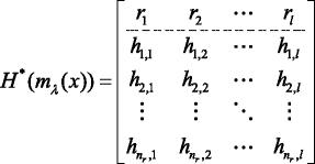 (28)
(28)where r1, r2, …, r3 are the soft-decision bits of the codeword C r , {hk,u|1 ≤ k ≤ n r , 1 ≤ u ≤ l} are the elements of Hbmin(m λ (x)) in GF(2).
-
2)
Replace each r u (1 ≤ u ≤ l) in H *(m λ (x)) with their absolute values to form a new matrix , adjust the positions of the columns in to make the first row in is ranked from the lowest to the highest and record the indexes. The absolute values of {r u |1 ≤ u ≤ l} denote the reliabilities of the received soft-decision bits. As shown in Equation 29, and i 1, i 2, ⋯, i l are the column indexes of in H*(m λ (x)).
 (29)
(29) -
3)
Transform by elementary row operations to make the last n r elements of the first column in has only one “1” at the top, as shown in Equation 30. The first row does not join the elementary transformations.
 (30)
(30)


This transformation limits the influences of the most unreliable decision bit to only one syndrome element. Furthermore, we continue the elementary transformation on to limit the numbers of “1” in the following n r –1 columns to one (except the first row), as shown in Equation 31.
When the left bottom n r × n r area becomes an indent matrix, stop the operation. Then the last n r rows in H r *(m λ (x)) form a new matrix. We recover its original column orders and call it Hbmin_ a(m λ (x)). Because the transformation is elementary, the relationship Hbmin_ a(m λ (x)) × C r = 0 in the hard decision situations still exists if C r is a valid codeword. So we can calculate the probability P r [S H (k) = 0] according to Hbmin_ a(m λ (x)). This replacement reduces the influences of the n r most unreliable decision bits.
In this paper, we assume that the transmitter is sending a binary sequence of codewords and using a binary phase shift keying (BPSK) modulation, i.e. let +1 and −1 be the modulated symbols of 0 and 1. The modulation operation from code bit c to modulated symbol s could be written as s = 1 – 2c, and we assume that the propagation channel is a binary symmetry channel which is corrupted by an additive white Gaussian noise (AWGN). For each configuration, the information symbols in the codes are randomly chosen. A received symbol r could be expressed as r = s + w, where w is the AWGN.
According to the previous assumptions, s is an equally probable binary random variable and
The noise w follows a normal distribution with the probability density function (PDF)
So the conditional PDF of r is
where is the variance of the noise.
For a given received bit r, we can obtain the following conditional probabilities:
Let r = [r1, r2, …,r n , rn+1, …] be a received soft-decision vector corresponding to the random modulated vector s = [s1, s2, …, s n , sn + 1, …]. We now calculate the conditional probabilities of s1 ⊕ s2 = + 1 and s1 ⊕ s2 = −1. According to the mapping operation defined by s = 1–2c, we have
Similarly, we can calculate the conditional probabilities of s1 ⊕ s2 ⊕ s3 = + 1 and s1 ⊕ s2 ⊕ s3 = −1 as follow:
We define the XOR-SUM operation as and assume that the conditional probabilities of XOR-SUM can be expressed as Equation 41:
Then, we have
According to the induction principle, the expression of the conditional probabilities in Equation 41 turns out to be true, and could be simplified as follows:
By employing Equation 44, we can calculate the probability P r [S H (k) = 0] as follows:
where w k is the number of ones in the k th row of the adapted minimal binary parity-check matrix Hbmin_a(m λ (x)), u v represents the position of the v th non-zero element in the k th row of Hbmin_a(m λ (x)). and are the u v th modulated symbol on the transmitter and the corresponding soft-decision output on the receiver, respectively.
In shortened code cases, a codeword with block length l and shortened length l s can be obtained by choosing the last l elements from a codeword which has a regular length (l + l s ) as follows:
where the first l s elements of C w are zeros. Therefore, we can simply obtain the minimal parity-check matrices of the shortened codes by deleting the first l s columns of Hbmin(m λ (x)).
4.2 Recognition of generator polynomials
After the code length and synchronization position estimation, the extension field degree m corresponding to the being recognized code can also be obtained. Then we can list the minimal polynomials over GF(2m) and find out which ones are factors of the generator polynomial. These minimal polynomials can also be recognized according to the probabilities of syndromes equaling to zero.
In the procedure of the code length and synchronization position estimation, we have calculated the probability that a minimal polynomial is a factor of the received codeword polynomials. We assume that the estimated code length and extension field degree are l and m, the number of minimal polynomials over GF(2m) is q and m1(x), m2(x), …, m q (x) are the minimal polynomials over GF(2m).
According to Equation 45, we can calculate the k th syndrome for a given minimal parity-check matrix of Hbmin(m λ (x)). Equation 47 is the log-likelihood ratios (LLR) of P r [S H (k) = 0], where H = Hbmin(m λ (x)) is
And we propose to calculate a likelihood criterion (LC) of m λ (x)(1 ≤ i ≤ q) being a factor of the generator polynomial as follows:
where Hbmin_a(m λ (x)) is the adapted minimal parity-check matrix corresponding to the minimal polynomial m λ (x), M is the number of packets in the observed window W as shown in Figure 2, n r is the number of the rows in Hbmin_a(m λ (x)), is the LLR defined by Equation 47 and calculated at the j th block of the observed window W. According to Equation 48, we can calculate the LCs of all the minimal polynomials over GF(2m). By comparing the LCs, we can choose the minimal polynomials, LCs of which are obviously higher than others, as the estimated factors of the generator polynomial, then the generator polynomial is obtained.
However, we can test whether the product of several most likely minimal polynomials is a factor of the generator polynomial to increase the successful recognition rate, because according to the adaptive processing of the parity-check matrices, the more parity equations we consider, the more we are able to construct a parity matrix which is parsed on less reliable bits. For the convenience of automatic recognition using computer programs, we propose the procedure including the following steps to estimate the optimal parity-check matrix:
Step 1: Calculate the LCs to form a vector L:
Step 2: Rank the vector L from the highest to the lowest, in order to form a new vector L R as follows:
and record the indexes:
where λ ω (1 ≤ ω ≤ q) denotes the index of in L.
Step 3: Let ω increase from 1 to q, combine the binary minimal parity matrices for the minimal polynomials , in order to form H ω as follows:
After adaptive processing for H ω , calculate the LCs of H ω × C r = 0(1 ≤ ω ≤ q) by Equation 53 and obtain the LC vector L H as shown in Equation 54.
Step 4: Find the maximal element of L H , record the corresponding matrix
Step 5: According to Equations 49 and 50, we can find the polynomials and write the generator polynomial as follows:
But in our work, we find that some minimal polynomials are easily lost. These minimal polynomials have the minimal parity-check matrices with low rows, so the adaptive processing can only reduce the influence for low number of unreliable decision bits. For example, consider the following minimal polynomials corresponding to the elements α1, α9 and α0 in GF(26):
The degrees of m1(x), m2(x) and m3(x) are 6, 3, and 1, respectively. Therefore, the number of rows of the binary minimal parity-check matrices Hbmin(m1(x)), Hbmin(m2(x)) and Hbmin(m3(x)) corresponding to m1(x), m2(x) and m3(x) are also 6, 3, and 1, respectively. So Hbmin(m1(x)), Hbmin(m2(x)) and Hbmin(m3(x)) can limit the influences of 6, 3, 1 unreliable decision bits after adaptive processing, respectively. For m2(x) and m3(x), the LCs of Hbmin_ a(m2(x)) and Hbmin_ a(m3(x)), especially Hbmin_ a(m2(x)), may lower than the incorrect minimal polynomials when the signal-to-noise ratio (SNR) is low. In this case, the ranking of LCs in Equation 50 may not be correct, so the generator polynomial recognition is failed. To solve this problem, we can additionally combine these minimal parity-check matrices with obtained in Step 4 described previously and check whether the corresponding minimal polynomials are also factors of the generator polynomials. The details of the additional steps are listed below:
Step 6: List the binary minimal parity-check matrices over GF(2m) which have low rows: Hbmin(mL 1(x)), Hbmin(mL 2(x)),…, Hbmin(mL η(x)), here η represents the number of binary minimal parity-check matrices with low rows.
Step 7 Record and initialize a variable τ to be 1.
Step 8: Combine and Hbmin(m Lτ (x)) to form a new parity-check matrix as follow:
Step 9: If , let and .
Step 10: If τ = η, execute step 11; else, let τ = τ + 1 and go back to step 8.
Step 11: Output the newly obtained as the final estimation of the parity-check matrix and get the generator polynomials according to the minimal polynomials corresponding to .
5. General recognition procedure
In this section, we present the general procedure for the blind recognition of binary cyclic codes based on the principles proposed in the previous sections. Before the recognition, some prior information could help to estimate the possible range of the code length l. Then, we traverse all the possible values of code length l and codeword starting position t and choose the parameter pair (l, t) which maximizes the IDEF defined in Equation 21 to be the estimated code length and block synchronization position. Note that to get the minimal polynomials for each code length l over an extension field GF(2m), we must know the field exponent m of the code. For an ordinary binary cyclic code, its code length is 2m − 1, while the code length l of a shortened code is , where l s is the shortened length. Therefore, the minimal value of the field exponent m for a code length l is the smallest integer k such that . The maximal value of m should be estimated with some prior information. For each code length l and synchronization position t, we traverse all the possible extension field degrees to calculate ∆H, and choose the maximum one as ∆H(l,t). After the code length estimation, we search for the minimal polynomials which are the factors of the generator polynomial by the algorithm described in section 4.2.
The general recognition procedure is listed below:
-
Step 1: According to some prior information, set the searching range of the code length l, i.e. set the minimal and maximal code length lmin and lmax.
-
Step 2: Design a window W which has a length L at least 10 × lmax, i.e. M = 10 in Figure 2.
-
Step 3: Full fill the window W with the received soft-decision bits.
-
Step 4: Set the code length l = lmin.
-
Step 5: Set the initial synchronization position t at 0, which is the starting position of W.
-
Step 6: Assume the code length is l and the synchronization position is t and calculate ∆H. Note that the window W has more than one assumed codewords, we calculate the ∆H on all the codewords and compute the mean of them as ∆H(l,t).
-
Step 7: If t < l, then let t = t + 1 and go back to step 6; if t = l, then jump to step 8.
-
Step 8: If l < l max , then let l = l + 1 and go back to step 5; if l = l max , then jump to step 9.
-
Step 9: Compare all the calculated ∆H(l,t), select the maximum one and get the corresponding values of l, t and m as the estimated code length, synchronization position and the degree of the GF of the recognized codes, respectively.
-
Step 10: Let the code length and synchronization position be the estimated parameters l and t, fetch M codewords from the observed window W. And list the minimal polynomials over GF(2m), which are m1(x), m2(x),…, m q (x).
-
Step 11: Calculate the LCs of the minimal polynomials over GF(2m) by Equations 47 and 48 for the M packets in W, and get the LC vector as shown in Equation 49.
-
Step 12: Recognize the generator polynomial follow the steps described in section 4.2.
Finally, we need a detection threshold to reject random data. When the received data stream is not encoded by binary cyclic codes, it can be considered that the data is random for all the coding parameters. The recognizer should give a report to reject the estimated parameters when the parity-check matrix is not likely enough.
We define the mean value of p′ j,λ for all the blocks in the observed window as follows:
where p′ j,λ is calculated by Equation 27 according to the recognized parity-check matrix , H in Equation 27 is the recognized parity-check matrix and n r denotes the number of rows of . As shown in Figure 4, the distributions of mean (p′ j,λ) for random data and coded data with correctly estimated coding parameters are separated. The distances between the two distributions are mainly determined by the noise level, the number of rows in , and the number of code blocks in the observed window. Experimentally, we propose the threshold δ to be about 0.6, in order to decide whether the data stream is random or not. After the estimation of the coding parameters, we calculate mean (p′ j,λ) for all complete code blocks in the observed window. If mean (p′ j,λ) is smaller than δ, we propose to reject the recognition result.

Probability density distribution of p ′ λ for the coded and random data.
6. Simulations
In this section, we show the efficiency of our proposed blind recognition algorithm by simulations. In the simulations, we assume that the searching range of the code length is 7 ~ 128 and the observed window contains N = 3,000 consecutive soft-decision bits from the BPSK demodulator. Meanwhile, we assume the data stream is corrupted by an AWGN on the channel.
When employing the proposed algorithm to recognize the BCH (63, 51) code, the simulation results for code length and synchronization position recognitions are shown in Figures 5, 6, 7 and 8. The SNR is E s /N 0 = 5 dB and corresponding BER is 10−2.19. Figure 5 shows the values of p′ λ defined in Equation 20 when l = 63 and m = 6, and the block synchronization is achieved. Figure 6 is the case of another l and m. It is shown in the two figures that when the code length and synchronization positions are correctly estimated, some minimal polynomials have higher probabilities to be factors of the received codeword polynomials. The obviously larger ones are calculated on the minimal polynomials which are factors of the generator polynomial. If the parameters are not correctly estimated, such feature will not exist. Figure 7 shows the IDEF ∆H for different code length l and synchronization position t, while the first bit of the observed window is the 40th bit of a codeword. When l = 63 and t = 23, the IDEF is the largest. Thus, we propose l = 63 and to be the estimation of the code length and synchronization positions, which are consistent with the simulation settings.

Values of p ′ λ under correct parameters.

Values of p ′ λ under incorrect parameters.

IDEF on different code length and synchronization positions.

FRP of code length and synchronization position recognization on different SNRs for several binary cyclic codes.
The performance of the algorithm is affected by the channel quality. In Figure 8, we draw the performance of the proposed algorithm when applied to code length recognitions of several different binary cyclic codes. The curves depict the false recognition probabilities (FRP) of the code length and synchronization position estimations on different SNRs. In Figure 8, we also compare the performance of our proposed recognition algorithm with the hard-decision-based RIDERS algorithm proposed in [16–18]. The PFR of our proposed algorithm fall rapidly when SNR increases, and it is much lower than that of the previous algorithms on each single SNR value.
After the code length estimation, the generator polynomial could be recognized by searching for the minimal polynomials which are factors of the generator polynomial according to the steps proposed in section 4.2. We assume that the data stream sent by the transmitter is coded by a cyclic code, the code length and information length of which are 63 and 36, respectively. We call it cyc (63, 36) code in this paper. The generator polynomial of the code is the product of the following minimal polynomials, which includes low-degree minimal polynomials:
The coded data is modulated by BPSK and corrupted by an AWGN with SNR Es/N0 = 1.5 dB, and the corresponding hard-decision BER is about 4 × 10⁻². The recognizing procedure is shown in Figures 9, 10 and 11.

Generator polynomial recognition of cyc (63, 36): original LCs.

Generator polynomial recognition of cyc (63, 36): sorted LCs.

FRP of generator polynomial recognization on different SNRs for several binary cyclic codes.
There are 13 minimal polynomials over GF(26), which are listed below:
Figure 9 shows the original LCs of different minimal polynomials over GF(26) to be factors of the codeword polynomials in the observed window. We rank the original LCs from the highest to the lowest, in order to form a new vector L R and record the index I (defined in Equation 51) as follows:
Then we let ω increase from 1 to 13, combine the binary minimal parity matrices for the minimal polynomials mI(1)(x)…mI(ω)(x), in order to form H ω by Equation 52, and calculate the LCs of H ω × C r = 0(1 ≤ ω ≤ q) by Equation 48. The LCs are shown in Figure 10. We can see that the LC of H4 is the highest. H4 is obtained by combining the minimal parity-check matrices Hbmin(m4(x)), Hbmin(m1(x)), Hbmin(m2(x)) and Hbmin(m3(x)). Furthermore, we list the low-degree minimal polynomials to check whether they are factors of the generator polynomial. The low-degree minimal polynomials are mL 1(x) = m5(x), mL 2(x) = m9(x), mL 3(x) = m11(x) and mL 4(x) = m13(x). We record LCmax = LC(H4) = 4,406.8 and execute the steps 8 ~ 10 described in section 4.2. Finally, we can obtain the values of LLR(H4,k)(1 ≤ k ≤ 4)) in Table 1.
It is obvious that LLR(H4,1) > 0.9 × LLR(H4) and LLR(H4,4) > 0.9 × LLR(H4,1). Therefore, H4,4 should be considered as the finally recognized parity-check matrix. According to section 4.2, H4,4 is obtained by combining the minimal parity-check matrices Hbmin(m4(x)), Hbmin(m1(x)), Hbmin(m2(x)), Hbmin(m3(x)), Hbmin(m5(x)) and Hbmin(m13(x)), so we can write the generator polynomial as follows:
The recognition result is accordant with the simulation settings.
Figure 11 shows the performance of the proposed generator polynomial recognition algorithm when applied to several different binary cyclic codes. The curves show the FRP on different noise levels. As Es/N0 rises, the curves fall rapidly. We also compare our proposed algorithm with the previous hard-decision-based recognition algorithms proposed in [16–18]. It shows that the recognition performance is improved obviously in soft-decision situations.
After the coding parameter recognition, an additional testing program checks whether the data is random. The principle is described in section 4.2. We list the error-rejection-probabilities (ERPs) for some binary cyclic codes and the error-acceptance probabilities (EAP) for random data in Table 2. The ERP level is much lower than the FRP. Especially when the noise level is low enough, the ERPs are nearly zeros. And all the random data is rejected, that is to say, nearly no recognized result on random data is accepted.
7. Conclusion
A blind recognition method for binary cyclic codes for non-cooperative communications and ACM in soft-decision situations is proposed. The code length and synchronization positions are estimated by checking the minimal parity-check matrices. After that, the whole check matrix and generator polynomial are reconstructed by searching which minimal polynomials are factors of the generator polynomial. The recognition method proposed in this paper is based on an earlier published RIDERS algorithm with some significant improvements. By calculating the probability that a minimal polynomial is a factor of the received codewords rather than checking whether an element in the extension field is a root of the codewords, we develop the RIDERS algorithm to soft-decision situations. To calculate the probability that a minimal polynomial is a factor of a received codeword, we adopt some algorithms and ideas introduced in soft-decision-based decoding methods and blind-frame-synchronization approaches for RS and BCH codes in the literatures. Although we have always a loss of performance when these algorithms are applied in cyclic codes while they are particularly well suited for LDPC codes, the algorithm proposed in this paper still has a previously better recognition performance for binary cyclic codes in a soft-decision situation than that in a hard-decision situation. And by the reliability-based adaptive processing, we reduce the influences of the most unreliability decision bits on the calculation of the syndromes, though the parity-check matrices of binary cyclic codes are not sparse. Moreover, the application field of the recognition method is extended to general binary cyclic codes in this paper, including shortened codes. To the best of our knowledge, this paper is the first publication in literature, which introduces an approach for complete-blind recognition of binary cyclic codes in soft-decision situations. Simulations show that our proposed blind recognition algorithm yields obviously better performance than that of the previous ones.
References
Choqueuse V, Marazin M, Collin L, Yao KC, Burel G: Blind reconstruction of linear space-time block codes: a likelihood-based approach. IEEE. Trans. Signal. Proc. 2010, 58(3):1290-1299.
Burel G, Gautier R: Blind estimation of encoder and interleaver characteristics in a non cooperative context. In Proceedings of IASTED International Conference on Communications, Internet and Information Technology. Scottsdale, AZ: ; 2003.
Marazin M, Gautier R, Burel G: Algebraic method for blind recovery of punctured convolutional encoders from an erroneous bitstream. IET. Signal. Proc. 2012, 6(2):122-131. 10.1049/iet-spr.2010.0343
Moosavi R, Larsson EG: A fast scheme for blind identification of channel codes. In Proceedings of the 54th GLOBECOM 2011. Houston: ; 2011.
Goldsmith AJ, Chua SG: Adaptive coded modulation for fading channels. IEEE. Tran. Commun. 1998, 46(5):595-602. 10.1109/26.668727
Marazin M, Gautier R, Burel G: Dual code method for blind identification of convolutional encoder for cognitive radio receiver design. In Proceedings of IEEE Globecom Workshops. Honolulu: ; 2009.
Wang F, Huang Z, Zhou Y: A method for blind recognition of convolution code based on Euclidean algorithm. In Proceedings of IEEE WiCom. Shanghai: ; 2007:21-25.
Dignel J, Hagenauer J: Parameter estimation of a convolutional encoder from noisy observations. In Proceedings of IEEE ISIT. Nice: ; 2007.
Marazin M, Gautier R, Burel G: Blind recovery of the second convolutional encoder of a turbo-code when its systematic outputs are punctured. Mil. Tech. Acad. Rev. 2009, XIX(2):213-232.
Yongguang Z: Blind recognition method for the turbo coding parameters. J. Xidian. Univ. 2011, 38(2):167-172.
Marazin M, Gautier R, Burel G: Blind recovery of k/n rate convolutional encoders in a noisy environment. EURASIP J. Wirel. Commun. Netw. 2011, 2011(168):1-9.
Cluzeau M: Block code reconstruction using iterative decoding techniques. In Proceedings of IEEE ISIT. Seattle: ; 2006.
Barbier J, Sicot G, Houcke S: Algebraic approach for the reconstruction of linear and convolutional error correcting codes. In Proceedings of World academy of science, engineering and technology. Venice, Italy: ; 2006.
Barbier J, Letessier J: Forward error correcting codes characterization based on rank properties. In Proceedings of International Conferences on Wireless Communications. Nanjing: ; 2009.
Junjun Z, Yanbin L: Blind recognition of low code-rate binary linear block codes. Radio. Eng. 2009, 39(1):19-22.
Niancheng W, Xiaojing Y: Recognition methods of BCH codes. Elec. Warfare. 2010, 2010(6):30-34.
Xiaojing Y, Niancheng W: Recognition method of BCH codes on roots information dispersion entropy and roots statistic. J. Detect. Contr. 2010, 32(3):69-73.
Xizai L, Zhiping H, Shaojing S: Fast recognition method of generator polynomial of BCH codes. J. Xidian. Univ. 2011, 38(6):187-191.
Lin S, Costello DJ: Costello, Reliability-based soft-decision decoding algorithms for linear block codes. In Error Control Coding: Fundamentals and Applications. 2nd edition. Englewood Cliffs, NJ: Pearson Pretice Hall; 2004:395-452.
Imad R, Sicot G, Houcke S: Blind frame synchronization for error correcting codes having a sparse parity check matrix. IEEE. Trans. Comm. 2009, 57(6):1574-1577.
Imad R, Houcke S: Theoretical analysis of a MAP based blind frame synchronizer. IEEE. Trans. Wireless. Commun. 2009, 8(11):5472-5476.
Imad R, Poulliat C, Houcke S, Gadat G: Blind frame synchronization of Reed-Solomon codes: non-binary vs. binary approach. In Proceedings of IEEE SPAWC 2010. Marrakech, Morocco: ; 2010.
Imad R, Houcke S, Jego C: Blind frame synchronization of product codes based on the adaptation of the parity check matrix. In Proceedings of IEEE ICC 2009. Dresden, Germany: ; 2009.
Lin S, Costello DJ: Linear block codes. In Error Control Coding: Fundamentals and Applications. 2nd edition. Englewood Cliffs, NJ: Pearson Pretice Hall; 2004:66-98.
Lin S, Costello DJ: Introduction to algebra. In Error Control Coding: Fundamentals and Applications. 2nd edition. Englewood Cliffs, NJ: Pearson Pretice Hall; 2004:25-65.
Jiang J, Narayanan KR: Iterative soft-input-soft-output decoding of Reed-Solomon codes by adapting the parity check matrix. IEEE. Trans. Infor. Theory. 2006, 52(8):3746-3756.
Acknowledgements
This paper was supported by the graduate innovation fund of the National University of Defence Technology. And we wish to thank the anonymous reviewers who helped to improve the quality of the paper.
Author information
Authors and Affiliations
Corresponding author
Additional information
Competing interests
The authors declare that they have no competing interests.
Authors’ original submitted files for images
Below are the links to the authors’ original submitted files for images.
Rights and permissions
Open Access This article is distributed under the terms of the Creative Commons Attribution 2.0 International License ( https://creativecommons.org/licenses/by/2.0 ), which permits unrestricted use, distribution, and reproduction in any medium, provided the original work is properly cited.
About this article
Cite this article
Jing, Z., Zhiping, H., Shaojing, S. et al. Blind recognition of binary cyclic codes. J Wireless Com Network 2013, 218 (2013). https://doi.org/10.1186/1687-1499-2013-218
Received:
Accepted:
Published:
DOI: https://doi.org/10.1186/1687-1499-2013-218