Training sequence design for MIMO channels: an application-oriented approach

Abstract

In this paper, the problem of training optimization for estimating a multiple-input multiple-output (MIMO) flat fading channel in the presence of spatially and temporally correlated Gaussian noise is studied in an application-oriented setup. So far, the problem of MIMO channel estimation has mostly been treated within the context of minimizing the mean square error (MSE) of the channel estimate subject to various constraints, such as an upper bound on the available training energy. We introduce a more general framework for the task of training sequence design in MIMO systems, which can treat not only the minimization of channel estimator’s MSE but also the optimization of a final performance metric of interest related to the use of the channel estimate in the communication system. First, we show that the proposed framework can be used to minimize the training energy budget subject to a quality constraint on the MSE of the channel estimator. A deterministic version of the 'dual’ problem is also provided. We then focus on four specific applications, where the training sequence can be optimized with respect to the classical channel estimation MSE, a weighted channel estimation MSE and the MSE of the equalization error due to the use of an equalizer at the receiver or an appropriate linear precoder at the transmitter. In this way, the intended use of the channel estimate is explicitly accounted for. The superiority of the proposed designs over existing methods is demonstrated via numerical simulations.

1 Introduction

An important factor in the performance of multiple antenna systems is the accuracy of the channel state information (CSI) [1]. CSI is primarily used at the receiver side for purposes of coherent or semicoherent detection, but it can be also used at the transmitter side, e.g., for precoding and adaptive modulation. Since in communication systems the maximization of spectral efficiency is an objective of interest, the training duration and energy should be minimized. Most current systems use training signals that are white, both spatially and temporally, which is known to be a good choice according to several criteria [2, 3]. However, in case that some prior knowledge on the channel or noise statistics is available, it is possible to tailor the training signal and to obtain a significantly improved performance. Especially, several authors have studied scenarios where long-term CSI in the form of a covariance matrix over the short-term fading is available. So far, most proposed algorithms have been designed to minimize the squared error of the channel estimate, e.g., [4–9]. Alternative design criteria are used in [5] and [10], where the channel entropy is minimized given the received training signal. In [11], the resulting capacity in the case of a single-input single-output (SISO) channel is considered, while [12] focuses on the pairwise error probability.

Herein, a generic context is described, drawing from similar techniques that have been recently proposed for training signal design in system identification [13–15]. This context aims at providing a unified theoretical framework that can be used to treat the MIMO training optimization problem in various scenarios. Furthermore, it provides a different way of looking at the aforementioned problem that could be adjusted to a wide variety of estimation-related problems in communication systems. First, we show how the problem of minimizing the training energy subject to a quality constraint can be solved, while a 'dual’ deterministic (average design) problem is considered^a. In the sequel, we show that by a suitable definition of the performance measure, the problem of optimizing the training for minimizing the channel MSE can be treated as a special case. We also consider a weighted version of the channel MSE, which relates to the well-known L-optimality criterion [16]. Moreover, we explicitly consider how the channel estimate will be used and attempt to optimize the end performance of the data transmission, which is not necessarily equivalent to minimizing the mean square error (MSE) of the channel estimate. Specifically, we study two uses of the channel estimate: channel equalization at the receiver using a minimum mean square error (MMSE) equalizer and channel inversion (zero-forcing precoding) at the transmitter, and derive the corresponding optimal training signals for each case. In the case of MMSE equalization, separate approximations are provided for the high and low SNR regimes. Finally, the resulting performance is illustrated based on numerical simulations. Compared to related results in the control literature, here, we directly design a finite length training signal and consider not only deterministic channel parameters but also a Bayesian channel estimation framework. A related pilot design strategy has been proposed in [17] for the problem of jointly estimating the frequency offset and the channel impulse response in single-antenna transmissions.

Implementing an adaptive choice of pilot signals in a practical system would require a feedback signalling overhead, since both the transmitter and the receiver have to agree on the choice of the pilots. Just as the previous studies in the area, the current paper is primarily intended to provide a theoretical benchmark on the resulting performance of such a scheme. Directly considering the end performance in the pilot design is a step into making the results more relevant. The data model used in [4–10] is based on the assumption that the channel is frequency flat but the noise is allowed to be frequency selective. Such a generalized assumption is relevant in systems that share spectrum with other radio interfaces using a narrower bandwidth and possibly in situations where channel coding introduces a temporal correlation in interfering signals. In order to focus on the main principles of our proposed strategy, we maintain this research line by using the same model in the current paper.

As a final comment, the novelty of this paper is on introducing the application-oriented framework as the appropriate context for training sequence design in communication systems. To this end, Hermitian form-like approximations of performance metrics are addressed here because they usually are good approximations of many performance metrics of interest, as well as for simplicity purposes and comprehensiveness of presentation. Although the ultimate performance metric in communications systems, namely the bit error rate (BER), would be of interest, its handling seems to be a challenging task and is reserved for future study. In this paper, we make an effort to introduce the application-oriented training design framework in the most illustrative and straightforward way.

This paper is organized as follows: Section 2 introduces the basic MIMO received signal model and specific assumptions on the structure of channel and noise covariance matrices. Section 3 presents the optimal channel estimators, when the channel is considered to be either a deterministic or a random matrix. Section 4 presents the application-oriented optimal training designs in a guaranteed performance context, based on confidence ellipsoids and Markov bound relaxations. Moreover, Section 5 focuses on four specific applications, namely that of MSE channel estimation, channel estimation based on the L-optimality criterion, and finally channel estimation for MMSE equalization and ZF precoding. Numerical simulations are provided in Section 6, while Section 7 concludes this paper.

1.1 Notations

Boldface (lowercase) is used for column vectors, x, and (uppercase) for matrices, X. Moreover, X^T, X^H, X^∗, and X^† denote the transpose, the conjugate transpose, the conjugate, and the Moore-Penrose pseudoinverse of X, respectively. The trace of X is denoted as tr(X) and A ≽ B means that A - B is positive semidefinite. vec(X) is the vector produced by stacking the columns of X, and (X)_i,j is the (i, j)-th element of X. [X]₊ means that all negative eigenvalues of X are replaced by zeros (i.e., [X]₊ ≽ 0). $\mathcal{C}\mathcal{N}(\bar{\mathbf{x}},\mathbf{Q})$ stands for circularly symmetric complex Gaussian random vectors, where $\bar{\mathbf{x}}$ is the mean and Q the covariance matrix. Finally, α! denotes the factorial of the non-negative integer α and mod (a, b) the modulo operation between the integers a, b.

2 System model

We consider a MIMO communication system with n _T antennas at the transmitter and n _R antennas at the receiver. The received signal at time t is modelled as

$$\mathbf{y}(t)=\mathbf{H}\mathbf{x}(t)+\mathbf{n}(t),$$

where $\mathbf{x}(t)\in {\mathbb{C}}^{n_T}$ and $\mathbf{y}(t)\in {\mathbb{C}}^{n_R}$ are the baseband representations of the transmitted and received signals, respectively. The impact of background noise and interference from adjacent communication links is represented by the additive term $\mathbf{n}(t)\in {\mathbb{C}}^{n_R}$. We will further assume that x(t) and n(t) are independent (weakly) stationary signals. The channel response is modeled by $\mathbf{H}\in {\mathbb{C}}^{n_R\times n_T}$, which is assumed constant during the transmission of one block of data and independent between blocks, that is, we are assuming frequency flat block fading. Two different models of the channel will be considered:

• (i) A deterministic model

• (ii) A stochastic Rayleigh fading model^b, i.e., $\text{vec}(\mathbf{H})\in \mathcal{C}\mathcal{N}(\mathbf{0},\mathbf{R})$, where, for mathematical tractability, we will assume that the known covariance matrix R possesses the Kronecker model used, e.g., in [7, 10]:

  $$\begin{array}{ll}\mathbf{R}& ={\mathbf{R}}_T^T\otimes {\mathbf{R}}_R\end{array}$$

  (1)

where ${\mathbf{R}}_T\in {\mathbb{C}}^{n_T\times n_T}$ and ${\mathbf{R}}_R\in {\mathbb{C}}^{n_R\times n_R}$ are the spatial covariance matrices at the transmitter and receiver side, respectively. This model has been experimentally verified in [18, 19] and further motivated in [20, 21].

We consider training signals of arbitrary length B, represented by $\mathbf{P}\in {\mathbb{C}}^{n_T\times B}$, whose columns are the transmitted signal vectors during training. Placing the received vectors in $\mathbf{Y}=\left[\mathbf{y}(1)\dots \mathbf{y}(B)\right]\in {\mathbb{C}}^{n_R\times B}$, we have

$$\mathbf{Y}=\mathbf{H}\mathbf{P}+\mathbf{N},$$

where $\mathbf{N}=\left[\mathbf{n}(1)\dots \mathbf{n}(B)\right]\in {\mathbb{C}}^{n_R\times B}$ is the combined noise and interference matrix.

Defining $\stackrel{\mathbf{~}}{\mathbf{P}}={\mathbf{P}}^T\otimes \mathbf{I}$, we can then write

$$\begin{array}{l}\text{vec}(\mathbf{Y})=\stackrel{\mathbf{~}}{\mathbf{P}}\text{vec}(\mathbf{H})+\text{vec}(\mathbf{N}).\end{array}$$

(2)

For example in [7, 10], we assume that $\text{vec}(\mathbf{N})\in \mathcal{C}\mathcal{N}(\mathbf{0},\mathbf{S})$, where the covariance matrix S also possesses a Kronecker structure:

$$\begin{array}{l}\mathbf{S}={\mathbf{S}}_Q^T\otimes {\mathbf{S}}_R.\end{array}$$

(3)

Here, ${\mathbf{S}}_Q\in {\mathbb{C}}^{B\times B}$ represents the temporal covariance matrix^c that is used to model the effect of temporal correlations in interfering signals, when the noise incorporates multiuser interference. Moreover, ${\mathbf{S}}_R\in {\mathbb{C}}^{n_R\times n_R}$ represents the received spatial covariance matrix that is mostly related with the characteristics of the receive array. The Kronecker structure (3) corresponds to an assumption that the spatial and temporal properties of N are uncorrelated.

The channel and noise statistics will be assumed known to the receiver during estimation. Statistics can often be achieved by long-term estimation and tracking [22]. For the data transmission phase, we will assume that the transmit signal {x(t)} is a zero-mean, weakly stationary process, which is both temporally and spatially white, i.e., its spectrum is Φ _x (ω) = λ _x I.

3 Channel matrix estimation

3.1 Deterministic channel estimation

The minimum variance unbiased (MVU) channel estimator for the signal model (2), subject to a deterministic channel (Assumption i) in Section 2, is given by [23]:

$$\text{vec}\left({\hat{\mathbf{H}}}_{\text{MVU}}\right)={\left({\stackrel{\mathbf{~}}{\mathbf{P}}}^H{\mathbf{S}}^{-1}\stackrel{\mathbf{~}}{\mathbf{P}}\right)}^{-1}{\stackrel{\mathbf{~}}{\mathbf{P}}}^H{\mathbf{S}}^{-1}\text{vec}(\mathbf{Y}).$$

(4)

This estimate has the distribution

$$\begin{array}{l}\text{vec}\left({\hat{\mathbf{H}}}_{\text{MVU}}\right)\in \mathcal{C}\mathcal{N}\left(\text{vec}(\mathbf{H}),{\mathcal{I}}_{\text{F,MVU}}^{-1}\right),\end{array}$$

(5)

where ${\mathcal{I}}_{\text{F,MVU}}$ is the inverse covariance matrix

$${\mathcal{I}}_{\text{F,MVU}}={\stackrel{\mathbf{~}}{\mathbf{P}}}^H{\mathbf{S}}^{-1}\stackrel{\mathbf{~}}{\mathbf{P}}.$$

(6)

From this, it follows that the estimation error $\tilde{\mathbf{H}}\triangleq {\hat{\mathbf{H}}}_{\text{MVU}}-\mathbf{H}$ will, with probability α, belong to the uncertainty set

$${\mathcal{D}}_D=\left\{\tilde{\mathbf{H}}:{\text{vec}}^H(\tilde{\mathbf{H}}){\mathcal{I}}_{\text{F,MVU}}\text{vec}(\tilde{\mathbf{H}})\le \frac{1}{2}{\chi }_{\alpha }^2(2n_T{n}_R)\right\},$$

(7)

where ${\chi }_{\alpha }^2(n)$ is the α percentile of the χ²(n) distribution [15].

3.2 Bayesian channel estimation

For the case of a stochastic channel model (Assumption ii) in Section 2, the posterior channel distribution becomes (see [23])

$$\text{vec}(\mathbf{H})|\mathbf{Y},\mathbf{P}\in \mathcal{C}\mathcal{N}\left(\text{vec}\left({\hat{\mathbf{H}}}_{\text{MMSE}}\right),{\mathbf{C}}_{\text{MMSE}}\right),$$

(8)

where the first and second moments are

$$\begin{array}{l}\text{vec}\left({\hat{\mathbf{H}}}_{\text{MMSE}}\right)={\left({\mathbf{R}}^{-1}+{\stackrel{\mathbf{~}}{\mathbf{P}}}^H{\mathbf{S}}^{-1}\stackrel{\mathbf{~}}{\mathbf{P}}\right)}^{-1}{\stackrel{\mathbf{~}}{\mathbf{P}}}^H{\mathbf{S}}^{-1}\text{vec}(\mathbf{Y}),\\ {\mathbf{C}}_{\text{MMSE}}={\left({\mathbf{R}}^{-1}+{\stackrel{\mathbf{~}}{\mathbf{P}}}^H{\mathbf{S}}^{-1}\stackrel{\mathbf{~}}{\mathbf{P}}\right)}^{-1}.\end{array}$$

(9)

Thus, the estimation error $\tilde{\mathbf{H}}\triangleq {\hat{\mathbf{H}}}_{\text{MMSE}}-\mathbf{H}$ will, with probability α, belong to the uncertainty set

$${\mathcal{D}}_B=\left\{\tilde{\mathbf{H}}:{\text{vec}}^H(\tilde{\mathbf{H}}){\mathcal{I}}_{\text{F,MMSE}}\text{vec}(\tilde{\mathbf{H}})\le \frac{1}{2}{\chi }_{\alpha }^2(2n_T{n}_R)\right\},$$

(10)

where ${\mathcal{I}}_{\text{F,MMSE}}\triangleq {\mathbf{C}}_{\text{MMSE}}^{-1}$ is the inverse covariance matrix in the MMSE case [15].

4 Application-oriented optimal training design

In a communication system, an estimate of the channel, say $\hat{\mathbf{H}}$, is needed at the receiver to detect the data symbols and may also be used at the transmitter to improve the performance. Let $J(\tilde{\mathbf{H}},\mathbf{H})$ be a scalar measure of the performance degradation at the receiver due to the estimation error $\tilde{\mathbf{H}}$ for a channel H. The objective of the training signal design is then to ensure that the resulting channel estimation error $\tilde{\mathbf{H}}$ is such that

$$J(\tilde{\mathbf{H}},\mathbf{H})\le \frac{1}{\gamma }$$

(11)

for some parameter γ > 0, which we call accuracy. In our settings, (11) cannot be typically ensured, since the channel estimation error is Gaussian-distributed (see (5) and (8)) and, therefore, can be arbitrarily large. However, for the MVU estimator (4), we know that, with probability $\alpha ,\tilde{\mathbf{H}}$ will belong to the set ${\mathcal{D}}_D$ defined in (7). Thus, we are led to training signal designs which guarantee (11) for all channel estimation errors $\tilde{\mathbf{H}}\in {\mathcal{D}}_D$. One training design problem that is based on this concept is to minimize the required transmit energy budget subject to this constraint

$$\begin{array}{c}\text{DGPP}:\underset{\mathbf{P}\in {\mathbb{C}}^{n_T\times B}}{\text{minimize}}\text{tr}(\mathbf{P}{\mathbf{P}}^H)\\ \text{s.t.}J(\tilde{\mathbf{H}},\mathbf{H})\le \frac{1}{\gamma }\forall \tilde{\mathbf{H}}\in {\mathcal{D}}_D.\end{array}$$

(12)

Similarly, for the MMSE estimator in Subsection 3.2, the corresponding optimization problem is given as follows:

$$\begin{array}{l}\text{SGPP}:\underset{\mathbf{P}\in {\mathbb{C}}^{n_T\times B}}{\text{minimize}}\text{tr}\left(\mathbf{P}{\mathbf{P}}^H\right)\\ \text{s.t.}J(\tilde{\mathbf{H}},\mathbf{H})\le \frac{1}{\gamma }\forall \tilde{\mathbf{H}}\in {\mathcal{D}}_B,\end{array}$$

(13)

where ${\mathcal{D}}_B$ is defined in (10). We will call (12) and (13) as the deterministic guaranteed performance problem (DGPP) and the stochastic guaranteed performance problem (SGPP), respectively. An alternative dual problem is to maximize the accuracy γ subject to a constraint $\mathcal{P}>0$ on the transmit energy budget. For the MVU estimator, this can be written as

$$\begin{array}{l}\text{DMPP}:\underset{\mathbf{P}\in {\mathbb{C}}^{n_T\times B}}{\text{maximize}}\gamma \\ \text{s.t.}J(\tilde{\mathbf{H}},\mathbf{H})\le \frac{1}{\gamma }\forall \tilde{\mathbf{H}}\in {\mathcal{D}}_D,\\ \text{tr}\left(\mathbf{P}{\mathbf{P}}^H\right)\le \mathcal{P}.\end{array}$$

(14)

We will call this problem as the deterministic maximized performance problem (DMPP). The corresponding Bayesian problem will be denoted as the stochastic maximized performance problem (SMPP). We will study the DGPP/SGPP in detail in this contribution, but the DMPP/SMPP can be treated in similar ways. In fact, Theorem 3 in [24] suggests that the solutions to the DMPP/SMPP are the same as for DGPP/SGPP, save for a scaling factor.

The existing work on optimal training design for MIMO channels are, to the best of the authors knowledge, based upon standard measures on the quality of the channel estimate, rather than on the quality of the end use of the channel. The framework presented in this section can be used to treat the existing results as special cases. Additionally, if an end performance metric is optimized, the DGPP/SGPP and DMPP/SMPP formulations better reflect the ultimate objective of the training design. This type of optimal training design formulations has already been used in the control literature, but mainly for large sample sizes [13, 14, 25, 26], yielding an enhanced performance with respect to conventional estimation-theoretic approaches. A reasonable question is to examine if such a performance gain can be achieved in the case of training sequence design for MIMO channel estimation, where the sample sizes would be very small.

Remark.

Ensuring (11) can be translated into a chance constraint of the for

$$\text{Pr}\left\{J(\tilde{\mathbf{H}},\mathbf{H})\le \frac{1}{\gamma }\right\}\ge 1-\epsilon$$

(15)

for some ε ∈ [0, 1]. Problems (12), (13), and (14) correspond to a convex relaxation of this chance constraint based on confidence ellipsoids [27], as we show in the next subsection.

4.1 Approximating the training design problems

A key issue regarding the above training signal design problems is their computational tractability. In general, they are highly non-linear and non-convex. In the sequel, we will nevertheless show that using some approximations, the corresponding optimization problems for certain applications of interest can be convexified. In addition, these approximations will show that DGPP and SGPP are very closely related. In particular, we will show that the performance metric for these applications can be approximated by

$$\begin{array}{l}J(\tilde{\mathbf{H}},\mathbf{H})\approx {\text{vec}}^H(\tilde{\mathbf{H}}){\mathcal{I}}_{\text{adm}}\text{vec}(\tilde{\mathbf{H}}),\end{array}$$

(16)

where the Hermitian positive definite matrix ${\mathcal{I}}_{\text{adm}}$ can be written in Kronecker product form as ${\mathcal{I}}_T^T\otimes {\mathcal{I}}_R$ for some matrices ${\mathcal{I}}_T$ and ${\mathcal{I}}_R$. This means that we can approximate the set $\{\tilde{\mathbf{H}}:J(\tilde{\mathbf{H}},\mathbf{H})\le 1/\gamma \}$ of all admissible estimation errors $\tilde{\mathbf{H}}$ by a (complex) ellipsoid in the parameter space [15]:

$$\begin{array}{l}{\mathcal{D}}_{\text{adm}}=\{\tilde{\mathbf{H}}:{\text{vec}}^H(\tilde{\mathbf{H}})\gamma {\mathcal{I}}_{\text{adm}}\text{vec}(\tilde{\mathbf{H}})\le 1\}.\end{array}$$

(17)

Consequently, the DGPP (12) can be approximated by

$$\begin{array}{l}\text{ADGPP}:\underset{\mathbf{P}\in {\mathbb{C}}^{n_T\times B}}{\text{minimize}}\text{tr}\left(\mathbf{P}{\mathbf{P}}^H\right)\\ \text{s.t.}{\mathcal{D}}_D\subseteq {\mathcal{D}}_{\text{adm}}.\end{array}$$

(18)

We call this problem the approximative DGPP (ADGPP). Both ${\mathcal{D}}_D$ and ${\mathcal{D}}_{\text{adm}}$ are level sets of quadratic functions of the channel estimation error. Rewriting (7) so that we have the same level as in (17), we obtain

$${\mathcal{D}}_D=\left\{\tilde{\mathbf{H}}:{\text{vec}}^H(\tilde{\mathbf{H}})\frac{2{\mathcal{I}}_{\text{F,MVU}}}{{\chi }_{\alpha }^2(2n_T{n}_R)}\text{vec}(\tilde{\mathbf{H}})\le 1\right\}.$$

Comparing this expression with (17) gives that ${\mathcal{D}}_D\subseteq {\mathcal{D}}_{\text{adm}}$ if and only if

$$\frac{2{\mathcal{I}}_{\text{F,MVU}}}{{\chi }_{\alpha }^2(2n_T{n}_R)}\succcurlyeq \gamma {\mathcal{I}}_{\text{adm}}$$

(for a more general result, see [15], Theorem 3.1).

When ${\mathcal{I}}_{\text{adm}}$ has the form ${\mathcal{I}}_{\text{adm}}={\mathcal{I}}_T^T\otimes {\mathcal{I}}_R$, with ${\mathcal{I}}_T\in {\mathbb{C}}^{n_T\times n_T}$ and ${\mathcal{I}}_R\in {\mathbb{C}}^{n_R\times n_R}$, the ADGPP (18) can then be written as

$$\begin{array}{l}\begin{array}{l}\underset{\mathbf{P}\in {\mathbb{C}}^{n_T\times B}}{\text{minimize}}\text{tr}\left(\mathbf{P}{\mathbf{P}}^H\right)\\ \text{s.t.}\underset{{\mathcal{I}}_{\text{F,MVU}}}{\underbrace{{\stackrel{\mathbf{~}}{\mathbf{P}}}^H{\mathbf{S}}^{-1}\stackrel{\mathbf{~}}{\mathbf{P}}}}\succcurlyeq \frac{\gamma {\chi }_{\alpha }^2(2n_T{n}_R)}{2}{\mathcal{I}}_T^T\otimes {\mathcal{I}}_R.\end{array}\end{array}$$

(19)

Similarly, by observing that ${\mathcal{D}}_{\text{adm}}$ only depends on the channel estimation error, and following the derivations above, the SGPP can be approximated by the following formulation

$$\begin{array}{l}\begin{array}{l}\underset{\mathbf{P}\in {\mathbb{C}}^{n_T\times B}}{\text{minimize}}\text{tr}\left(\mathbf{P}{\mathbf{P}}^H\right)\\ \text{s.t.}\underset{{\mathcal{I}}_{\text{F,MMSE}}}{\underbrace{{\mathbf{R}}^{-1}+{\stackrel{\mathbf{~}}{\mathbf{P}}}^H{\mathbf{S}}^{-1}\stackrel{\mathbf{~}}{\mathbf{P}}}}\succcurlyeq \frac{\gamma {\chi }_{\alpha }^2(2n_T{n}_R)}{2}{\mathcal{I}}_T^T\otimes {\mathcal{I}}_R.\end{array}\end{array}$$

(20)

We call the last problem approximative SGPP (ASGPP).

Remarks.

• 1. The approximation (16) is not possible for the performance metric of every application. Several examples that this is possible are presented in Section 5. Therefore, in some applications, different convex approximations of the corresponding performance metrics may have to be found.

• 2. The quality of the approximation (16) is characterized by its corresponding tightness to the true performance metric. For our purposes, when the tightness of the aforementioned approximation is acceptable, such an approximation will be desirable for two reasons. First, it corresponds to a Hermitian form, therefore offering nice mathematical properties and tractability. Additionally, the constraint ${\mathcal{D}}_D\subseteq {\mathcal{D}}_{\text{adm}}$ can be efficiently handled.

• 3. The sizes of ${\mathcal{D}}_D$ and ${\mathcal{D}}_{\text{adm}}$ critically depend on the parameter α. In practice, requiring α to have a value close to 1 corresponds to adequately representing the uncertainty set in which (approximately) all possible channel estimation errors lie.

4.2 The deterministic guaranteed performance problem

The problem formulations for ADGPP and ASGPP in (19) and (20), respectively, are similar in structure. The solutions to these problems (and to other approximative guaranteed performance problems) can be obtained from the following general theorem, which has not previously been available in the literature, to the best of our knowledge:

Theorem 1.

Consider the optimization problem

$$\begin{array}{l}\begin{array}{l}\underset{\mathbf{P}\in {\mathbb{C}}^{n\times N}}{\text{minimize}}\text{tr}\left(\mathbf{P}{\mathbf{P}}^H\right)\\ \mathrm{s.t.}\mathbf{P}{\mathbf{A}}^{-1}{\mathbf{P}}^H\succcurlyeq \mathbf{B}\end{array}\end{array}$$

(21)

where$\mathbf{A}\in {\mathbb{C}}^{N\times N}$is Hermitian positive definite, $\mathbf{B}\in {\mathbb{C}}^{n\times n}$is Hermitian positive semidefinite, and N ≥ rank (B). An optimal solution to (21) is

$$\begin{array}{l}{\mathbf{P}}^{\text{opt}}={\mathbf{U}}_B{\mathbf{D}}_P{\mathbf{U}}_A^H,\end{array}$$

(22)

where${\mathbf{D}}_P\in {\mathbb{C}}^{n\times N}$is a rectangular diagonal matrix with$\sqrt{{({\mathbf{D}}_A)}_{1,1}{({\mathbf{D}}_B)}_{1,1}}\dots \sqrt{{({\mathbf{D}}_A)}_{m,m}{({\mathbf{D}}_B)}_{m,m}}$on the main diagonal. Here, m = min(n, N), while U _A and U _B are unitary matrices that originate from the eigendecompositions of A and B, respectively, i.e.,

$$\begin{array}{ll}\mathbf{A}& ={\mathbf{U}}_A{\mathbf{D}}_A{\mathbf{U}}_A^H\\ \mathbf{B}& ={\mathbf{U}}_B{\mathbf{D}}_B{\mathbf{U}}_B^H\end{array}$$

(23)

and D _A , D _B are real-valued diagonal matrices, with their diagonal elements sorted in ascending and descending order, respectively, that is, 0 < (D _A )_1,1 ≤ … ≤ (D _A )_N,Nand (D _B )_1,1 ≥ … ≥ (D _B )_n,n ≥ 0.

If the eigenvalues of A and B are distinct and strictly positive, then the solution (22) is unique up to the multiplication of the columns of U _A and U _B by complex unit-norm scalars.

Proof.

The proof is given in Appendix 7. □

By the right choice of A and B, Theorem 1 will solve the ADGPP in (19). This is shown by the next theorem (recall that we have assumed that $\mathbf{S}={\mathbf{S}}_Q^T\otimes {\mathbf{S}}_R$).

Theorem 2.

Consider the optimization problem

$$\begin{array}{l}\begin{array}{l}\underset{\mathbf{P}\in {\mathbb{C}}^{n_T\times B}}{\text{minimize}}\text{tr}\left(\mathbf{P}{\mathbf{P}}^H\right)\\ \mathrm{s.t.}{\stackrel{\mathbf{~}}{\mathbf{P}}}^H{({\mathbf{S}}_Q^T\otimes {\mathbf{S}}_R)}^{-1}\stackrel{\mathbf{~}}{\mathbf{P}}\succcurlyeq c{\mathcal{I}}_T^T\otimes {\mathcal{I}}_R,\end{array}\end{array}$$

(24)

where$\stackrel{\mathbf{~}}{\mathbf{P}}={\mathbf{P}}^T\otimes \mathbf{I}$, ${\mathbf{S}}_Q\in {\mathbb{C}}^{B\times B}$, ${\mathbf{S}}_R\in {\mathbb{C}}^{n_R\times n_R}$are Hermitian positive definite, ${\mathcal{I}}_T\in {\mathbb{C}}^{n_T\times n_T}$, ${\mathcal{I}}_R\in {\mathbb{C}}^{n_R\times n_R}$are Hermitian positive semidefinite, and c is a positive constant.

If $B\ge \text{rank}({\mathcal{I}}_T)$, this problem is equivalent to (21) in Theorem 1 for A = S _Q and$\mathbf{B}=c{\lambda }_{\text{max}}\left({\mathbf{S}}_R{\mathcal{I}}_R\right){\mathcal{I}}_T$, where λ_max(·) denotes the maximum eigenvalue.

Proof.

The proof is given in Appendix 7. □

4.3 The stochastic guaranteed performance problem

We will see that Theorem 1 can be also used to solve the ASGPP in (20). In order to obtain closed-form solutions, we need some equality relation between the Kronecker blocks of $\mathbf{R}={\mathbf{R}}_T^T\otimes {\mathbf{R}}_R$ and of either $\mathbf{S}={\mathbf{S}}_Q^T\otimes {\mathbf{S}}_R$ or ${\mathcal{I}}_{\text{adm}}={\mathcal{I}}_T^T\otimes {\mathcal{I}}_R$. For instance, it can be R _R  = S _R , which may be satisfied if the receive antennas are spatially uncorrelated or if the signal and interference are received from the same main direction (see [7] for details on the interpretations of these assumptions).

The solution to ASGPP in (20) is given by the next theorem.

Theorem 3.

Consider the optimization problem

$$\begin{array}{l}\begin{array}{l}\underset{\mathbf{P}\in {\mathbb{C}}^{n_T\times B}}{\text{minimize}}\text{tr}\left(\mathbf{P}{\mathbf{P}}^H\right)\\ \mathrm{s.t.}{\mathbf{R}}^{-1}+{\stackrel{\mathbf{~}}{\mathbf{P}}}^H{\mathbf{S}}^{-1}\stackrel{\mathbf{~}}{\mathbf{P}}\succcurlyeq c{\mathcal{I}}_T^T\otimes {\mathcal{I}}_R,\end{array}\end{array}$$

(25)

where$\stackrel{\mathbf{~}}{\mathbf{P}}={\mathbf{P}}^T\otimes \mathbf{I}$, $\mathbf{R}={\mathbf{R}}_T^T\otimes {\mathbf{R}}_R$, and$\mathbf{S}={\mathbf{S}}_Q^T\otimes {\mathbf{S}}_R$. Here, ${\mathbf{R}}_T\in {\mathbb{C}}^{n_T\times n_T}$, ${\mathbf{R}}_R\in {\mathbb{C}}^{n_R\times n_R}$, ${\mathbf{S}}_Q\in {\mathbb{C}}^{B\times B}$, ${\mathbf{S}}_R\in {\mathbb{C}}^{n_R\times n_R}$are Hermitian positive definite, ${\mathcal{I}}_T\in {\mathbb{C}}^{n_T\times n_T}$, ${\mathcal{I}}_R\in {\mathbb{C}}^{n_R\times n_R}$are Hermitian positive semidefinite, and c is a positive constant.

• If R _R  = S _R and$B\ge \text{rank}\left({\left[c{\lambda }_{\text{max}}\left({\mathbf{S}}_R{\mathcal{I}}_R\right){\mathcal{I}}_T-{\mathbf{R}}_T^{-1}\right]}_{+}\right)$, then the problem is equivalent to (21) in Theorem 1 for A = S _Q and$\mathbf{B}={\left[c{\lambda }_{\text{max}}({\mathbf{S}}_R{\mathcal{I}}_R){\mathcal{I}}_T-{\mathbf{R}}_T^{-1}\right]}_{+}$.

• If${\mathbf{R}}_R^{-1}={\mathcal{I}}_R$and$B\ge \text{rank}\left({\left[c{\mathcal{I}}_T-{\mathbf{R}}_T^{-1}\right]}_{+}\right)$, then the problem is equivalent to (21) in Theorem 1 for A = S _Q and$\mathbf{B}={\lambda }_{\text{max}}({\mathbf{S}}_R{\mathcal{I}}_R){\left[c{\mathcal{I}}_T-{\mathbf{R}}_T^{-1}\right]}_{+}$.

• If${\mathbf{R}}_T^{-1}={\mathcal{I}}_T$and$B\ge \text{rank}\left({\mathcal{I}}_T\right)$, then the problem is equivalent to (21) in Theorem 1 for A = S _Q and$\mathbf{B}={\lambda }_{\text{max}}\left({\mathbf{S}}_R{\left[c{\mathcal{I}}_R-{\mathbf{R}}_R\right]}_{+}\right){\mathcal{I}}_T$.

Proof.

The proof is given in Appendix 3. □

The mathematical difference between ADGPP and ASGPP is the R^-1 term that appears in the constraint of the latter. This term has a clear impact on the structure of the optimal ASGPP training matrix.

It is also worth noting that the solution for R _R  = S _R requires $B\ge \text{rank}({[c{\lambda }_{\text{max}}({\mathbf{S}}_R{\mathcal{I}}_R){\mathcal{I}}_T-{\mathbf{R}}_T^{-1}]}_{+})$ which means that solutions can be achieved also for B < n _T (i.e., when only the B < n _T strongest eigendirections of the channel are excited by training). In certain cases, e.g., when the interference is temporally white (S _Q  = I), it is optimal to have $B=\text{rank}({[c{\lambda }_{\text{max}}({\mathbf{S}}_R{\mathcal{I}}_R){\mathcal{I}}_T-{\mathbf{R}}_T^{-1}]}_{+})$ as larger B will not decrease the training energy usage, cf.[9].

4.4 Optimizing the average performance

Except from the previously presented training designs, the application-oriented design can be alternatively given in the following deterministic dual context. If H is considered to be deterministic, then we can set up the following optimization problem

$$\begin{array}{l}\begin{array}{ll}\underset{\mathbf{P}\in {\mathbb{C}}^{n_T\times B}}{\text{minimize}}& {\mathbb{E}}_{\tilde{\mathbf{H}}}\left\{J(\tilde{\mathbf{H}},\mathbf{H})\right\}\\ \hfill \mathrm{s.t.}\hfill & \text{tr}(\mathbf{P}{\mathbf{P}}^H)\le \mathcal{P}.\hfill \end{array}\end{array}$$

(26)

Clearly, for the MVU estimator

$${\mathbb{E}}_{\tilde{\mathbf{H}}}\left\{J(\tilde{\mathbf{H}},\mathbf{H})\right\}=\text{tr}\left\{{\mathcal{I}}_{\text{adm}}{({\stackrel{\mathbf{~}}{\mathbf{P}}}^H{\mathbf{S}}^{-1}\stackrel{\mathbf{~}}{\mathbf{P}})}^{-1}\right\},$$

so problem (26) is solved by the following theorem.

Theorem 4.

Consider the optimization problem

$$\begin{array}{l}\begin{array}{ll}\underset{\mathbf{P}\in {\mathbb{C}}^{n_T\times B}}{\text{minimize}}& \text{tr}\left\{{\mathcal{I}}_{\text{adm}}{({\stackrel{\mathbf{~}}{\mathbf{P}}}^H{\mathbf{S}}^{-1}\stackrel{\mathbf{~}}{\mathbf{P}})}^{-1}\right\}\\ \hfill \mathrm{s.t.}\hfill & \text{tr}(\mathbf{P}{\mathbf{P}}^H)\le \mathcal{P},\end{array}\end{array}$$

(27)

where${\mathcal{I}}_{\text{adm}}={\mathcal{I}}_T^T\otimes {\mathcal{I}}_R$as before. Set${\mathcal{I}}_T^{\prime }={\mathcal{I}}_T^T={\mathbf{U}}_T{\mathbf{D}}_T{\mathbf{U}}_T^H$and${\mathbf{S}}_Q^{\prime }={\mathbf{S}}_Q^T={\mathbf{U}}_Q{\mathbf{D}}_Q{\mathbf{U}}_Q^H$. Here, ${\mathbf{U}}_T\in {\mathbb{C}}^{n_T\times n_T}$, ${\mathbf{U}}_Q\in {\mathbb{C}}^{B\times B}$are unitary matrices and D _T , D _Q are diagonal n _T  × n _T and B  × B matrices containing the eigenvalues of${\mathcal{I}}_T^{\prime }$and${\mathbf{S}}_Q^{\prime }$in descending and ascending order, respectively. Then, the optimal training matrix P equals${\left({\mathbf{U}}_T{\mathbf{D}}_P{\mathbf{U}}_Q^H\right)}^{\ast }$, where D _P is an n _T  × B diagonal matrix with main diagonal entries equal to${({\mathbf{D}}_P)}_{i,i}=\sqrt{\mathcal{P}\sqrt{{\alpha }_i}/{\sum }_{j=1}^{n_T}\sqrt{{\alpha }_j}},i=1,2,\dots ,n_T(B\ge n_T)$ and α _i  = (D _T )_i,i(D _Q )_i,i, i = 1, 2, …, n _T with the aforementioned ordering.

Proof.

The proof is given in Appendix 7. □

Remarks.

• 1. In the general case of a non-Kronecker-structured ${\mathcal{I}}_{\text{adm}}$, the training can be obtained using numerical methods like the semidefinite relaxation approach described in [28].

• 2. If ${\mathcal{I}}_{\text{adm}}$ depends on H, then in order to implement this design, the embedded H in ${\mathcal{I}}_{\text{adm}}$ may be replaced by a previous channel estimate. This implies that this approach is possible whenever the channel variations allow for such a design. This observation also applies to the designs in the previous subsections (see also [24, 29], where the same issue is discussed for other system identification applications).

The corresponding performance criterion for the case of the MMSE estimator is given by

$${\mathbb{E}}_{\tilde{\mathbf{H}},\mathbf{H}}\left\{J(\tilde{\mathbf{H}},\mathbf{H})\right\}=\text{tr}\left\{{\mathcal{I}}_{\text{adm}}{({\mathbf{R}}^{-1}+{\stackrel{\mathbf{~}}{\mathbf{P}}}^H{\mathbf{S}}^{-1}\stackrel{\mathbf{~}}{\mathbf{P}})}^{-1}\right\}.$$

In this case, we can derive closed form expressions for the optimal training under assumptions similar to those made in Theorem 3. We therefore have the following result:

Theorem 5.

Consider the optimization problem

$$\begin{array}{l}\begin{array}{ll}\underset{\mathbf{P}\in {\mathbb{C}}^{n_T\times B}}{\text{minimize}}& \text{tr}\left\{{\mathcal{I}}_{\text{adm}}{({\mathbf{R}}^{-1}+{\stackrel{\mathbf{~}}{\mathbf{P}}}^H{\mathbf{S}}^{-1}\stackrel{\mathbf{~}}{\mathbf{P}})}^{-1}\right\}\\ \hfill \mathrm{s.t.}\hfill & \text{tr}(\mathbf{P}{\mathbf{P}}^H)\le \mathcal{P}\hfill \end{array}\end{array}$$

(28)

where${\mathcal{I}}_{\text{adm}}={\mathcal{I}}_T^T\otimes {\mathcal{I}}_R$as before. Set${\mathbf{S}}_Q^{\prime }={\mathbf{S}}_Q^T={\mathbf{V}}_Q{\mathit{\Lambda }}_Q{\mathbf{V}}_Q^H$. Here, we assume that${\mathbf{V}}_Q\in {\mathbb{C}}^{B\times B}$is a unitary matrix and Λ _Q a diagonal B × B matrix containing the eigenvalues of${\mathbf{S}}_Q^{\prime }$in arbitrary order. Assume also that${\mathbf{R}}_T^{\prime }={\mathbf{R}}_T^T$with eigenvalue decomposition${\mathbf{U}}_T^{\prime }{\mathit{\Lambda }}_T^{\prime }{\mathbf{U}}_T^{\mathrm{\prime H}}$. The diagonal elements of${\mathit{\Lambda }}_T^{\prime }$are assumed to be arbitrarily ordered. Then, we have the following cases:

• R _R  = S _R : We further discriminate two cases

  • $${\mathcal{I}}_T=\mathbf{I}$$

    : Then the optimal training is given by a straightforward adaptation of Proposition 2 in[8].

  • $${\mathbf{R}}_T^{-1}={\mathcal{I}}_T$$

    : Then, the optimal training matrix P equals${\left({\mathbf{U}}_T^{\prime }({\pi }_{\text{opt}}){\mathbf{D}}_P{\mathbf{V}}_Q^H({\varpi }_{\text{opt}})\right)}^{\ast }$, where π_opt, ϖ_optstand for the optimal orderings of the eigenvalues of${\mathbf{R}}_T^{\prime }$and${\mathbf{S}}_Q^{\prime }$, respectively. These optimal orderings are determined by Algorithm 1 in Appendix 5. Additionally, define the parameter m_∗as in Equation 69 (see Appendix 5). Assuming in the following that, for simplicity of notation, ${({\mathit{\Lambda }}_T^{\prime })}_{i,i}$’s and (Λ _Q )_i,i’s have the optimal ordering, the optimal (D _P )_j,j, j = 1, 2, …, m_∗are given by the expression

    $$\begin{array}{l}\sqrt{\frac{\mathcal{P}+{\sum }_{i=1}^{m_{\ast }}\frac{{({\mathit{\Lambda }}_Q)}_{i,i}}{{({\mathit{\Lambda }}_T^{\prime })}_{i,i}}}{\sum _{i=1}^{m_{\ast }}\sqrt{\frac{{({\mathit{\Lambda }}_Q)}_{i,i}}{{({\mathit{\Lambda }}_T^{\prime })}_{i,i}}}}\sqrt{\frac{{({\mathit{\Lambda }}_Q)}_{j,j}}{{({\mathit{\Lambda }}_T^{\prime })}_{j,j}}}-\frac{{({\mathit{\Lambda }}_Q)}_{j,j}}{{({\mathit{\Lambda }}_T^{\prime })}_{j,j}}},\end{array}$$

    while (D _P )_j,j = 0 for j = m_∗ + 1, …, n _T .

Proof.

The proof is given in Appendix 5. □

Remarks. Two interesting additional cases complementing the last theorem are the following:

• 1. If the modal matrices of R _R and S _R are the same, ${\mathcal{I}}_T=\mathbf{I}$ and ${\mathcal{I}}_R=\mathbf{I}$, then the optimal training is given by [9].

• 2. In any other case (e.g., if R _R  ≠ S _R ), the training can be found using numerical methods like the semidefinite relaxation approach described in [28]. Note again that this approach can also handle general ${\mathcal{I}}_{\text{adm}}$, not necessarily expressed as ${\mathcal{I}}_T^T\otimes {\mathcal{I}}_R$.

As a general conclusion, the objective function of the dual deterministic problems presented in this subsection can be shown to correspond to Markov bound approximations of the chance constraint (15), as these approximations have been described in [27], namely

$$\begin{array}{l}\text{Pr}\left\{J(\tilde{\mathbf{H}},\mathbf{H})\ge \frac{1}{\gamma }\right\}\le \gamma \mathbb{E}\left\{J(\tilde{\mathbf{H}},\mathbf{H})\right\}\le \epsilon \end{array}$$

According to the analysis in [27], these approximations should be tighter than the approximations based on confidence ellipsoids presented in Subsections 4.1, 4.2, and 4.3 for practically relevant values of ε.

5 Applications

5.1 Optimal training for channel estimation

We now consider the channel estimation problem in its standard context, where the performance metric of interest is the MSE of the corresponding channel estimator. Optimal linear estimators for this task are given by (4) and (9). The performance metric of interest is

$$J(\tilde{\mathbf{H}},\mathbf{H})={\text{vec}}^H(\tilde{\mathbf{H}})\text{vec}(\tilde{\mathbf{H}}),$$

which corresponds to ${\mathcal{I}}_{\text{adm}}=\mathbf{I}$, i.e., to ${\mathcal{I}}_T=\mathbf{I}$ and ${\mathcal{I}}_R=\mathbf{I}$. The ADGPP and ASGPP are given by (19) and (20), respectively, with the corresponding substitutions. Their solutions follow directly from Theorems 2 and 3, respectively. To the best of the authors’ knowledge, such formulations for the classical MIMO training design problem are presented here for the first time. Furthermore, solutions to the standard approach of minimizing the channel MSE subject to a constraint on the training energy budget are provided by Theorems 4 and 5 as special cases.

Remark.

Although the confidence ellipsoid and Markov bound approximations are generally different [27], in the simulation section, we show that their performance is almost identical for reasonable operating γ-regimes in the specific case of standard channel estimation.

5.2 Optimal training for the L-optimality criterion

Consider now a performance metric of the form

$$J_W(\tilde{\mathbf{H}},\mathbf{H})={\text{vec}}^H(\tilde{\mathbf{H}})\mathbf{W}\text{vec}(\tilde{\mathbf{H}}),$$

for some positive semidefinite weighting matrix W. Assume also that W = W₁ ⊗ W₂ for some positive semidefinite matrices W₁, W₂. Taking the expected value of this performance metric with respect to either $\tilde{\mathbf{H}}$ or both $\tilde{\mathbf{H}}$ and H leads to the well-known L-optimality criterion for optimal experiment design in statistics [16]. In this case, ${\mathcal{I}}_T={\mathbf{W}}_1^T$ and ${\mathcal{I}}_R={\mathbf{W}}_2$. In the context of MIMO communication systems, such a performance metric may arise, e.g., if we want to estimate the MIMO channel having some deficiencies in either the transmit and/or the receive antenna arrays. The simplest case would be both W₁ and W₂ being diagonal with non-zero entries in the interval [0,1], W₁ representing the deficiencies in the transmit antenna array and W₂ in the receive array. More general matrices can be considered if we assume cross-couplings between the transmit and/or receive antenna elements.

Remark.

The numerical approach of [28] mentioned after Theorems 4 and 5 can handle general weighting matrices W, not necessarily Kronecker-structured.

5.3 Optimal training for channel equalization

In this subsection, we consider the problem of estimating a transmitted signal sequence {x(t)} from the corresponding received signal sequence {y(t)}. Among a wide range of methods that are available [30, 31], we will consider the MMSE equalizer, and for mathematical tractability, we will approximate it by the non-causal Wiener filter. Note that for reasonably long block lengths, the MMSE estimate becomes similar to the non-causal Wiener filter [32]. Thus, the optimal training design based on the non-causal Wiener filter should also provide good performance when using an MMSE equalizer.

5.3.1 Equalization using exact channel state information

Let us first assume that H is available. In this ideal case and with the transmitted signal being weakly stationary with spectrum Φ _x , the optimal estimate of the transmitted signal x(t) from the received observations of y(t) can be obtained according to

$$\widehat{\mathbf{x}}(t;\mathbf{H})=\mathbf{F}(q;\mathbf{H})\mathbf{y}(t),$$

(29)

where q is the unit time shift operator, [q x(t) = x(t + 1)], and the non-causal Wiener filter F(e^jω;H) is given by

$$\begin{array}{l}\mathbf{F}(e^{\mathrm{j\omega }};\mathbf{H})={\mathbf{\Phi }}_{\mathit{\text{xy}}}(\omega ){\mathbf{\Phi }}_y^{-1}(\omega )\\ ={\mathbf{\Phi }}_x(\omega ){\mathbf{H}}^H{\left(\mathbf{H}{\mathbf{\Phi }}_x(\omega ){\mathbf{H}}^H+{\mathbf{\Phi }}_n(\omega )\right)}^{-1}.\end{array}$$

(30)

Here, Φ _xy (ω) = Φ _x (ω)H^H denotes the cross-spectrum between x(t) and y(t), and

$${\mathbf{\Phi }}_y(\omega )=\mathbf{H}{\mathbf{\Phi }}_x(\omega ){\mathbf{H}}^H+{\mathbf{\Phi }}_n(\omega )$$

(31)

is the spectral density of y(t). Using our assumption that Φ _x (ω) = λ _x I, we obtain the simplified expression

$$\begin{array}{ll}\mathbf{F}(e^{\mathrm{j\omega }};\mathbf{H})& ={\mathbf{H}}^H{\left(\mathbf{H}{\mathbf{H}}^H+{\mathbf{\Phi }}_n(\omega )/{\lambda }_x\right)}^{-1}.\end{array}$$

(32)

Remark.

Assuming non-singularity of Φ _n (ω) for every ω, the MMSE equalizer is applicable for all values of the pair (n _T , n _R ).

5.3.2 Equalization using a channel estimate

Consider now the situation where the exact channel H is unavailable, but we only have an estimate $\hat{\mathbf{H}}$. When we replace H by its estimate in the expressions above, the estimation error for the equalizer will increase. While the increase in the bit error rate would be a natural measure of the quality of the channel estimate $\hat{\mathbf{H}}$, for simplicity, we consider the total MSE of the difference, $\widehat{\mathbf{x}}(t;\mathbf{H}+\tilde{\mathbf{H}})-\widehat{\mathbf{x}}(t;\mathbf{H})=\mathit{\Delta }(q;\tilde{\mathbf{H}},\mathbf{H})\mathbf{y}(t)$ (note that $\hat{\mathbf{H}}=\mathbf{H}+\tilde{\mathbf{H}}$), using the notation $\mathit{\Delta }(q;\tilde{\mathbf{H}},\mathbf{H})\triangleq \mathbf{F}(q;\mathbf{H}+\tilde{\mathbf{H}})-\mathbf{F}(q;\mathbf{H})$. In view of this, we will use the channel equalization (CE) performance metric

$$\begin{array}{ll}{J}_{\text{CE}}(\tilde{\mathbf{H}},\mathbf{H})& =\mathbb{E}\left\{{\left[\mathit{\Delta }(q;\tilde{\mathbf{H}},\mathbf{H})\mathbf{y}(t)\right]}^H\left[\mathit{\Delta }(q;\tilde{\mathbf{H}},\mathbf{H})\mathbf{y}(t)\right]\right\}\\ =\mathbb{E}\left\{\text{tr}\left(\left[\mathit{\Delta }(q;\tilde{\mathbf{H}},\mathbf{H})\mathbf{y}(t)\right]{\left[\mathit{\Delta }(q;\tilde{\mathbf{H}},\mathbf{H})\mathbf{y}(t)\right]}^H\right)\right\}\\ =\frac{1}{2\pi }\underset{-\pi }{\overset{\pi }{\int }}\text{tr}\left(\mathit{\Delta }(e^{\mathrm{j\omega }};\tilde{\mathbf{H}},\mathbf{H}){\mathbf{\Phi }}_y(\omega ){\mathit{\Delta }}^H(e^{\mathrm{j\omega }};\tilde{\mathbf{H}},\mathbf{H})\right)d\omega .\end{array}$$

(33)

We see that the poorer the accuracy of the estimate, the larger the performance metric $J_{\text{CE}}(\tilde{\mathbf{H}},\mathbf{H})$ and, thus, the larger the performance loss of the equalizer. Therefore, this performance metric is a reasonable candidate to use when formulating our training sequence design problem. Indeed, the Wiener equalizer based on the estimate $\hat{\mathbf{H}}=\mathbf{H}+\tilde{\mathbf{H}}$ of H can be deemed to have a satisfactory performance if $J_{\text{CE}}(\tilde{\mathbf{H}},\mathbf{H})$ remains below some user-chosen threshold. Thus, we will use J_CE as J in problems (12) and (13). Though these problems are not convex, we show in Appendix 1 how they can be convexified, provided some approximations are made.

Remarks.

• 1. The excess MSE $J_{\mathit{\text{CE}}}(\tilde{\mathbf{H}},\mathbf{H})$ quantifies the distance of the MMSE equalizer using the channel estimate $\hat{\mathbf{H}}$ over the clairvoyant MMSE equalizer, i.e., the one using the true channel. This performance metric is not the same as the classical MSE in the equalization context, where the difference $\widehat{\mathbf{x}}(t;\mathbf{H}+\tilde{\mathbf{H}})-\mathbf{x}(t)$ is considered instead of $\widehat{\mathbf{x}}(t;\mathbf{H}+\tilde{\mathbf{H}})-\widehat{\mathbf{x}}(t;\mathbf{H})$. However, since in practice the best transmit vector estimate that can be attained is the clairvoyant one, the choice of $J_{\text{CE}}(\tilde{\mathbf{H}},\mathbf{H})$ is justified. This selection allows for a performance metric approximation given by (16).

• 2. There are certain cases of interest, where $J_{\text{CE}}(\tilde{\mathbf{H}},\mathbf{H})$ approximately coincides with the classical equalization MSE. Such a case occurs when n _R  ≥ n _T , H is full column rank and the SNR is high during data transmission.

5.4 Optimal training for zero-forcing precoding

Apart from receiver side channel equalization, as another example of how to apply the channel estimate we consider point-to-point zero-forcing (ZF) precoding, also known as channel inversion [33]. Here, the channel estimate is fed back to the transmitter, and its (pseudo-)inverse is used as a linear precoder. The data transmission is described by

$$\mathbf{y}(t)=\mathbf{H}\mathbf{\Psi }\mathbf{x}(t)+\mathbf{v}(t),$$

where the precoder is $\mathbf{\Psi }={\hat{\mathbf{H}}}^{\mathrm{†}}$, i.e., $\mathbf{\Psi }={\hat{\mathbf{H}}}^H{(\hat{\mathbf{H}}{\hat{\mathbf{H}}}^H)}^{-1}$ if we limit ourselves to the practically relevant case n _T  ≥ n _R and assume that $\hat{\mathbf{H}}$ is full rank. Note that x(t) is an n _R  × 1 vector in this case, but the transmitted vector is Ψ x(t), which is n _T  × 1.

Under these assumptions and following the same strategy and notation as in Appendix 1, we get

$$\begin{array}{l}\mathbf{y}(t;\hat{\mathbf{H}})-\mathbf{y}(t;\mathbf{H})=\mathbf{H}{\hat{\mathbf{H}}}^{\mathrm{†}}\mathbf{x}(t)+\mathbf{v}-(\mathbf{H}{\mathbf{H}}^{\mathrm{†}}\mathbf{x}(t)+\mathbf{v})\\ =(\hat{\mathbf{H}}{\hat{\mathbf{H}}}^{\mathrm{†}}-\tilde{\mathbf{H}}{\hat{\mathbf{H}}}^{\mathrm{†}}-\mathbf{I})\mathbf{x}(t)\simeq -\tilde{\mathbf{H}}{\mathbf{H}}^{\mathrm{†}}\mathbf{x}(t).\end{array}$$

(34)

Consequently, a quadratic approximation of the cost function is given by

$$\begin{array}{ll}{J}_{\text{ZF}}(\tilde{\mathbf{H}},\mathbf{H})& =\mathbb{E}\left\{{\left[\mathbf{y}(t;\hat{\mathbf{H}})-\mathbf{y}(t;\mathbf{H})\right]}^H\left[\mathbf{y}(t;\hat{\mathbf{H}})-\mathbf{y}(t;\mathbf{H})\right]\right\}\\ \simeq {\lambda }_x{\text{vec}}^H(\tilde{\mathbf{H}})\left({({\mathbf{H}}^{\mathrm{†}}{({\mathbf{H}}^{\mathrm{†}})}^H)}^T\otimes \mathbf{I}\right)\text{vec}(\tilde{\mathbf{H}})\\ ={\text{vec}}^H(\tilde{\mathbf{H}})({\mathcal{I}}_T^T\otimes {\mathcal{I}}_R)\text{vec}(\tilde{\mathbf{H}}),\end{array}$$

(35)

if we define ${\mathcal{I}}_T={\lambda }_x{\mathbf{H}}^{\mathrm{†}}{({\mathbf{H}}^{\mathrm{†}})}^H={\lambda }_x{\mathbf{H}}^H{(\mathbf{H}{\mathbf{H}}^H)}^{-2}\mathbf{H}$ and ${\mathcal{I}}_R=\mathbf{I}$.

Remark.

The cost functions of (27) and (28) reveal the fact that any performance-oriented training design is a compromise between the strict channel estimation accuracy and the desired accuracy related to the end performance metric at hand. Caution is needed to identify cases where the performance-oriented design may severely degrade the channel estimation accuracy, annihilating all gains from such a design. In the case of ZF precoding, if n _T  > n _R , ${\mathcal{I}}_T$ will have rank at most n _R yielding a training matrix P with only n _R active eigendirections. This is in contrast to the secondary target, which is the channel estimation accuracy. Therefore, we expect ADGPP, ASGPP, and the approaches in Subsection 4.4 to behave abnormally in this case. Thus, we propose the performance-oriented design only when n _T  = n _R in the context of the ZF precoding.

6 Numerical examples

The purpose of this section is to examine the performance of optimal training sequence designs and compare them with existing methods. For the channel estimation MSE figure, we plot the normalized MSE (NMSE), i.e., $\mathbb{E}(\parallel \mathbf{H}-\hat{H}{\parallel }^2/\parallel \mathbf{H}{\parallel }^2)$, versus the accuracy parameter γ. In all figures, fair comparison among the presented schemes is ensured via training energy equalization. Additionally, the matrices R _T , R _R , S _Q , S _R follow the exponential model, that is, they are built according to

$${(\mathbf{R})}_{i,j}=r{j-i}^{},j\ge i,$$

(36)

where r is the (complex) normalized correlation coefficient with magnitude ρ = |r| < 1. We choose to examine the high correlation scenario for all the presented schemes. Therefore, in all plots, |r| = 0.9 for all matrices R _T , R _R , S _Q , S _R . Additionally, the transmit SNR during data transmission is chosen to be 15 dB, when channel equalization and ZF precoding are considered. High SNR expressions are therefore used for optimal training sequence designs. Since the optimal pilot sequences depend on the true channel, we have for these two applications additionally assumed that the channel changes from block to block according to the relationship H _i  = H_i-1 + μ E _i , where E _i has the same Kronecker structure as H, and it is completely independent from H_i-1. The estimated H_i-1 is used in the pilot design. The value of μ is 0.01.

In Figure 1, the channel estimation NMSE performance versus the accuracy γ is presented for three different schemes. The scheme 'ASGPP’ is the optimal Wiener filter together with the optimal guaranteed performance training matrix described in Subsection 5.1. 'Optimal MMSE’ is the scheme presented in [9], which solves the optimal training problem for the vectorized MMSE, operating on vec(Y). This solution is a special case in the statement of Theorem 5 for ${\mathcal{I}}_{\text{adm}}=\mathbf{I}$, i.e., ${\mathcal{I}}_T=\mathbf{I}$ and ${\mathcal{I}}_R=\mathbf{I}$. Finally, the scheme 'White training’ corresponds to the use of the vectorized MMSE filter at the receiver, with a white training matrix, i.e., one having equal singular values and arbitrary left and right singular matrices. This scheme is justified when the receiver knows the involved channel and noise statistics but does not want to sacrifice bandwidth to feedback the optimal training matrix to the transmitter. This scheme is also justifiable in fast fading environments. In Figure 1, we assume that R _R  = S _R , and we implement the corresponding optimal training design for each scheme. ASGPP is implemented first for a certain value of γ, and the rest of the schemes are forced to have the same training energy. The Optimal MMSE in [9] and ASGPP schemes have the best and almost identical MSE performance. This indicates that for the problem of training design with the classical channel estimation MSE, the confidence ellipsoid relaxation of the chance constraint and the relaxation based on the Markov bound in Subsection 4.4 deliver almost identical performances. This verifies the validity of the approximations in this paper for the classical channel estimation problem.

Figure 1

Channel estimation NMSE based on Subsection 5.1 with R _R  =  S _R . n _T  = 4, n _R  = 2, B = 6, a (%) = 99.

Figures 2 and 3 demonstrate the L-optimality average performance metric E{J _W } versus γ. Figure 2 corresponds to the L-optimality criterion based on MVU estimators and Figure 3 is based on MMSE estimators. In Figure 2, the scheme 'MVU’ corresponds to the optimal training for channel estimation when the MVU estimator is used. This training is given by Theorem 4 for ${\mathcal{I}}_{\text{adm}}=\mathbf{I}$, i.e., ${\mathcal{I}}_T=\mathbf{I}$ and ${\mathcal{I}}_R=\mathbf{I}$. 'MVU in Subsection 4.4’ is again the MVU estimator based on the same theorem but for the correct ${\mathcal{I}}_{\text{adm}}$. The scheme 'MMSE in Subsection 4.4’ is given by the numerical solution mentioned below Theorem 5, since W₁ is different than the cases where a closed form solution is possible. Figures 2 and 3 clearly show that both the confidence ellipsoid and Markov bound approximations are better than the optimal training for standard channel estimation. Therefore, for this problem, the application-oriented training design is superior compared to training designs with respect to the quality of the channel estimate.

Figure 2

L-optimality criterion with arbitrary but positive semidefinite W ₁ , W ₂ for the MVU estimator. n _T  = 6, n _R  = 6, B = 8, a (%) = 99.

Figure 3

L-optimality criterion with arbitrary but positive semidefinite W ₁ , W ₂ for the MMSE estimator with R _R  = S _R . n _T  = 3, n _R  = 3, B = 4, a (%) = 99.

Figure 4 demonstrates the performance of optimal training designs for the MMSE estimator in the context of MMSE channel equalization. We assume that R _R  ≠ S _R , since the high SNR expressions for ${\mathcal{I}}_{\text{adm}}$ in the context of MMSE channel equalization in Appendix 1 indicate that ${\mathcal{I}}_T=\mathbf{I}$ for this application and according to Theorem 5 the optimal training corresponds to the optimal training for channel estimation in [8]. We observe that the curves almost coincide. Moreover, it can be easily verified that for MMSE channel equalization with the MVU estimator, the optimal training designs given by Theorems 2 and 4 differ slightly only in the optimal power loading. These observations essentially show that the optimal training designs for the MVU and MMSE estimators in the classical channel estimation setup are nearly optimal for the application of MMSE channel equalization. This relies on the fact that for this particular application, ${\mathcal{I}}_T=\mathbf{I}$ in the high data transmission SNR regime.

Figure 4

MMSE channel equalization with R _R ≠ S _R . n _T  = 4, n _R  = 2, B = 6, SNR = 15 dB, μ = 0.01.

Figures 5 and 6 present the corresponding performances in the case of the ZF precoding. The descriptions of the schemes are as before. In Figure 6, we assume that R _R  = S _R . The superiority of the application-oriented designs for the ZF precoding application is apparent in these plots. Here, ${\mathcal{I}}_T\ne \mathbf{I}$ and this is why the optimal training for the channel estimate works less well in this application. Moreover, the ASGPP is plotted for γ ≥ 0 dB, since for γ ≤ -5 dB all the eigenvalues of $\mathbf{B}={\left[c{\lambda }_{\text{max}}\left({\mathbf{S}}_R{\mathcal{I}}_R\right){\mathcal{I}}_T-{\mathbf{R}}_T^{-1}\right]}_{+}$ are equal to zero for this particular set of parameters defining Figure 6.

Figure 5

ZF precoding based on Subsection 5.4 for the MVU estimator.${\mathcal{I}}_{\text{adm}}$ is based on a previous channel estimate. n _T  = 5, n _R  = 5, B = 7, SNR = 15 dB, a (%) = 99, μ = 0.01.

Figure 6

ZF precoding MSE based on Subsection 5.4 for the MMSE estimator with R _R  = S _R .${\mathcal{I}}_{\text{adm}}$ is based on a previous channel estimate. n _T  = 4, n _R  = 4, B = 6, SNR = 15 dB, μ = 0.01, a (%) = 99.

Figure 7 presents an outage plot in the context of the L-optimality criterion for the MVU estimator. We assume that γ = 1. We plot Pr{ J _W  > 1 / γ} versus the training power. This plot indirectly verifies that the confidence ellipsoid relaxation of the chance constraint given by the scheme ASGPP is not as tight as the Markov bound approximation given by the scheme MVU in Subsection 4.4.

Figure 7

Outage probability for the L-optimality criterion with the MVU estimator. n _T  = 6, n _R  = 6, B = 8, γ = 1. The accuracy parameter is γ = 1.

Finally, Figures 8 and 9 present the BER performance of the nearest neighbor rule applied to the signal estimates produced by the corresponding schemes in Figure 6. The used modulation is quadrature phase-shift keying (QPSK). The 'Clairvoyant’ scheme corresponds to the ZF precoder with perfect channel knowledge. The channel estimates have been obtained for γ = -10 and 0 dB, respectively. Even if the application-oriented estimates are not optimized for the BER performance metric, they lead to better performance than the Optimal MMSE scheme in [9] as is apparent in Figure 8. In Figure 9, the performances of all schemes approximately coincide. This is due to the fact that for γ = 5 dB, all channel estimates are very good, thus leading to symbol MSE performance differences that do not translate to the corresponding BER performances for the nearest neighbor decision rule.

Figure 8

BER performance using the signal estimates produced by the corresponding schemes in Figure 6 with R _R = S _R and γ = -10 dB.${\mathcal{I}}_{\text{adm}}$ is based on a previous channel estimate. n _T  = 4, n _R  = 4, B = 6, γ = -10 dB, μ = 0.01, a(%) = 99.

Figure 9

BER performance using the signal estimates produced by the corresponding schemes in Figure 6 with R _R =S _R and γ = 5 dB.${\mathcal{I}}_{\text{adm}}$ is based on a previous channel estimate. n _T  = 4, n _R  = 4, B = 6, γ = 5 dB, μ = 0.01, a(%) = 99.

7 Conclusions

In this contribution, we have presented a quite general framework for MIMO training sequence design subject to flat and block fading, as well as spatially and temporally correlated Gaussian noise. The main contribution has been to incorporate the objective of the channel estimation into the design. We have shown that by a suitable approximation of $J(\tilde{\mathbf{H}},\mathbf{H})$, it is possible to solve this type of problem for several interesting applications such as standard MIMO channel estimation, L-optimality criterion, MMSE channel equalization, and ZF precoding. For these problems, we have numerically demonstrated the superiority of the schemes derived in this paper. Additionally, the proposed framework is valuable since it provides a universal way of posing different estimation-related problems in communication systems. We have seen that it shows interesting promise for, e.g., ZF precoding, and it may yield even greater end performance gains in estimation problems related to communication systems, when approximations can be avoided, depending on the end performance metric at hand.

Endnotes

^a The word 'dual’ in this paper defers from the Lagrangian duality studied in the context of convex optimization theory (see [24] for more details on this type of duality).

^b For simplicity, we have assumed a zero-mean channel, but it is straightforward to extend the results to Rician fading channels, similar to [9].

^c We set the subscript Q to S _Q to highlight its temporal nature and the fact that its size is B × B. The matrices with subscript T in this paper share the common characteristic that they are n _T  × n _T , while those with subscript R are n _R  × n _R .

^d For a Hermitian positive semidefinite matrix A, we consider here that A^1/2 is the matrix with the same eigenvectors as A and eigenvalues as the square roots of the corresponding eigenvalues of A. With this definition of the square root of a Hermitian positive semidefinite matrix, it is clear that A^1/2 = A^H/2, leading to A = A^1/2A^H/2 = A^H/2A^1/2.

^e For easiness, we use the MATLAB notation in this table.

Appendix 1

Approximating the performance measure for MMSE channel equalization

In order to obtain the approximating set ${\mathcal{D}}_{\text{adm}}$, let us first denote the integrand in the performance metric (33) by

$$J^{\prime }(\omega ;\tilde{\mathbf{H}},\mathbf{H})=\text{tr}\left(\mathit{\Delta }(e{\mathrm{j\omega }}^{};\tilde{\mathbf{H}},\mathbf{H}){\mathbf{\Phi }}_y(\omega ){\mathit{\Delta }}^H(e{\mathrm{j\omega }}^{};\tilde{\mathbf{H}},\mathbf{H})\right).$$

(37)

In addition, let ≃ denote an equality in which only dominating terms with respect to $\left|\right|\tilde{\mathbf{H}}\left|\right|$ are retained. Then, using (32), we observe that

$$\begin{array}{l}\mathit{\Delta }(e{\mathrm{j\omega }}^{};\tilde{\mathbf{H}},\mathbf{H})=\mathbf{F}(e{\mathrm{j\omega }}^{};\mathbf{H}+\tilde{\mathbf{H}})-\mathbf{F}(e{\mathrm{j\omega }}^{};\mathbf{H})\\ \simeq {\lambda }_x{\tilde{\mathbf{H}}}^H{\mathbf{\Phi }}_y^{-1}-{\lambda }_x^2{\mathbf{H}}^H{\mathbf{\Phi }}_y^{-1}(\mathbf{H}{\tilde{\mathbf{H}}}^H+\tilde{\mathbf{H}}{\mathbf{H}}^H){\mathbf{\Phi }}_y^{-1}\\ ={\lambda }_x\left(\underset{=\mathbf{Q}}{\underbrace{\left(\mathbf{I}-{\lambda }_x{\mathbf{H}}^H{\mathbf{\Phi }}_y^{-1}\mathbf{H}\right)}}{\tilde{\mathbf{H}}}^H{\mathbf{\Phi }}_y^{-1}-{\lambda }_x{\mathbf{H}}^H{\mathbf{\Phi }}_y^{-1}\tilde{\mathbf{H}}{\mathbf{H}}^H{\mathbf{\Phi }}_y^{-1}\right),\end{array}$$

(38)

where we omitted the argument ω for simplicity. Inserting (38) in (37) results in the approximation

$$\begin{array}{ll}{J}^{\prime }(\omega ;\tilde{\mathbf{H}},\mathbf{H})& \simeq {\lambda }_x^2\text{tr}\left(\mathbf{Q}{\tilde{\mathbf{H}}}^H{\mathbf{\Phi }}_y^{-1}\tilde{\mathbf{H}}\mathbf{Q}\right.\\ +{\lambda }_x^2\left({\mathbf{H}}^H{\mathbf{\Phi }}_y^{-1}\tilde{\mathbf{H}}{\mathbf{H}}^H{\mathbf{\Phi }}_y^{-1}\mathbf{H}{\tilde{\mathbf{H}}}^H{\mathbf{\Phi }}_y^{-1}\mathbf{H}\right)\\ -{\lambda }_x\mathbf{Q}{\tilde{\mathbf{H}}}^H{\mathbf{\Phi }}_y^{-1}\mathbf{H}{\tilde{\mathbf{H}}}^H{\mathbf{\Phi }}_y^{-1}\mathbf{H}\\ \left.-{\lambda }_x{\mathbf{H}}^H{\mathbf{\Phi }}_y^{-1}\tilde{\mathbf{H}}{\mathbf{H}}^H{\mathbf{\Phi }}_y^{-1}\tilde{\mathbf{H}}\mathbf{Q}\right).\end{array}$$

(39)

To rewrite this into a quadratic form in terms of $\text{vec}(\tilde{\mathbf{H}})$, we use the facts that tr(A B) = tr(B A) = vec^T(A^T)vec(B) = vec^H(A^H)vec(B) and vec(A B C) = (C^T ⊗ A)vec(B) for matrices A, B, and C of compatible dimensions. Hence, we can rewrite (39) as

$$\begin{array}{l}{J}^{\prime }(\omega ;\tilde{\mathbf{H}},\mathbf{H})\simeq {\text{vec}}^H(\tilde{\mathbf{H}})[{\lambda }_x^2{{\mathbf{Q}}^2}^T\otimes {\mathbf{\Phi }}_y^{-1}]\text{vec}(\tilde{\mathbf{H}})\\ +{\text{vec}}^H(\tilde{\mathbf{H}})[{\lambda }_x^4{({\mathbf{H}}^H{\mathbf{\Phi }}_y^{-1}\mathbf{H})}^T\otimes {\mathbf{\Phi }}_y^{-1}\mathbf{H}{\mathbf{H}}^H{\mathbf{\Phi }}_y^{-1}]\text{vec}(\tilde{\mathbf{H}})\\ -{\text{vec}}^H(\tilde{\mathbf{H}})[{\lambda }_x^3{({\mathbf{\Phi }}_y^{-1}\mathbf{H}\mathbf{Q})}^T\otimes {\mathbf{\Phi }}_y^{-1}\mathbf{H}]\text{vec}({\tilde{\mathbf{H}}}^H)\\ -{\text{vec}}^H({\tilde{\mathbf{H}}}^H)[{\lambda }_x^3{(\mathbf{Q}{\mathbf{H}}^H{\mathbf{\Phi }}_y^{-1})}^T\otimes {\mathbf{H}}^H{\mathbf{\Phi }}_y^{-1}]\text{vec}(\tilde{\mathbf{H}}).\end{array}$$

(40)

In the next step, we introduce the permutation matrix Π defined such that $\text{vec}({\tilde{\mathbf{H}}}^T)=\mathbf{\Pi }\text{vec}(\tilde{\mathbf{H}})$ for every $\tilde{\mathbf{H}}$ to rewrite (40) as

$$\begin{array}{l}{J}^{\prime }(\omega ;\tilde{\mathbf{H}},\mathbf{H})\simeq {\text{vec}}^H(\tilde{\mathbf{H}})[{\lambda }_x^2{{\mathbf{Q}}^2}^T\otimes {\mathbf{\Phi }}_y^{-1}]\text{vec}(\tilde{\mathbf{H}})\\ +{\text{vec}}^H(\tilde{\mathbf{H}})[{\lambda }_x^4{({\mathbf{H}}^H{\mathbf{\Phi }}_y^{-1}\mathbf{H})}^T\otimes {\mathbf{\Phi }}_y^{-1}\mathbf{H}{\mathbf{H}}^H{\mathbf{\Phi }}_y^{-1}]\text{vec}(\tilde{\mathbf{H}})\\ -{\text{vec}}^H(\tilde{\mathbf{H}})[{\lambda }_x^3{({\mathbf{\Phi }}_y^{-1}\mathbf{H}\mathbf{Q})}^T\otimes {\mathbf{\Phi }}_y^{-1}\mathbf{H}]\mathbf{\Pi }\text{vec}({\tilde{\mathbf{H}}}^{\ast })\\ -{\text{vec}}^H({\tilde{\mathbf{H}}}^{\ast }){\mathbf{\Pi }}^T[{\lambda }_x^3{(\mathbf{Q}{\mathbf{H}}^H{\mathbf{\Phi }}_y^{-1})}^T\otimes {\mathbf{H}}^H{\mathbf{\Phi }}_y^{-1}]\text{vec}(\tilde{\mathbf{H}}).\end{array}$$

(41)

We have now obtained a quadratic form. Note indeed that the last two terms are just complex conjugates of each other and thus we can write them as two times their real part.

High SNR analysis

In order to obtain a simpler expression for ${\mathcal{I}}_{\text{adm}}$, we will assume high SNR in the data transmission phase. We consider the practically relevant case where rank(H) = min(n _T , nn _n R). Depending on the rank of the channel matrix H, we will have three different cases:

Case 1.

rank(H) = n _R  < n _T Under this assumption, it can be shown that both the first and the second terms on the right hand side of (41) contribute to ${\mathcal{I}}_{\text{adm}}$. We have $\mathbf{Q}\to {\mathbf{\Pi }}_{{\mathbf{H}}^H}^{\perp }$ and ${\lambda }_x{\mathbf{\Phi }}_y^{-1}\to {(\mathbf{H}{\mathbf{H}}^H)}^{-1}$ for high SNR. Here, and in what follows, we use Π _X  = X X^† to denote the orthogonal projection matrix on the range space of X and ${\mathbf{\Pi }}_{\mathbf{X}}^{\perp }=\mathbf{I}-{\mathbf{\Pi }}_{\mathbf{X}}$ to denote the projection on the nullspace of X^H. Moreover, ${\lambda }_x{\mathbf{H}}^H{\mathbf{\Phi }}_y^{-1}\mathbf{H}\to {\mathbf{\Pi }}_{{\mathbf{H}}^H}$ and ${\lambda }_x^2{\mathbf{\Phi }}_y^{-1}\mathbf{H}{\mathbf{H}}^H{\mathbf{\Phi }}_y^{-1}\to {(\mathbf{H}{\mathbf{H}}^H)}^{-1}$ for high SNR. As ${\mathbf{\Pi }}_{{\mathbf{H}}^H}^{\perp }+{\mathbf{\Pi }}_{{\mathbf{H}}^H}=\mathbf{I}$, summing the contributions from the first two terms in (41) finally gives the high SNR approximation

$${\mathcal{I}}_{\text{adm}}={\lambda }_x\mathbf{I}\otimes {(\mathbf{H}{\mathbf{H}}^H)}^{-1}.$$

(42)

Case 2.

rank(H) = n _R  = n _T For the non-singular channel case, the second term on the right hand side of (41) dominates. Here, we have ${\lambda }_x{\mathbf{H}}^H{\mathbf{\Phi }}_y^{-1}\mathbf{H}\to \mathbf{I}$ and ${\lambda }_x^2{\mathbf{\Phi }}_y^{-1}\mathbf{H}{\mathbf{H}}^H{\mathbf{\Phi }}_y^{-1}\to {(\mathbf{H}{\mathbf{H}}^H)}^{-1}$ for high SNR. Clearly, this results in the same expression for ${\mathcal{I}}_{\text{adm}}$ as in Case 1, namely

$${\mathcal{I}}_{\text{adm}}={\lambda }_x\mathbf{I}\otimes {(\mathbf{H}{\mathbf{H}}^H)}^{-1}.$$

(43)

Case 3.

rank(H) = n _T  < n _R In this case, the second term on the right hand side of (41) dominates. When rank(H) = n _T , we get ${\lambda }_x{\mathbf{H}}^H{\mathbf{\Phi }}_y^{-1}\mathbf{H}\to \mathbf{I}$ and ${\lambda }_x^2{\mathbf{\Phi }}_y^{-1}\mathbf{H}{\mathbf{H}}^H{\mathbf{\Phi }}_y^{-1}\to {\mathbf{\Phi }}_n^{-1/2}{\left[{\mathbf{\Phi }}_n^{-1/2}\mathbf{H}{\mathbf{H}}^H{\mathbf{\Phi }}_n^{-1/2}\right]}^{\mathrm{†}}{\mathbf{\Phi }}_n^{-1/2}$ for high SNR. Using these approximations finally gives the high SNR approximation

$$\begin{array}{l}{\mathcal{I}}_{\text{adm}}={\lambda }_x\mathbf{I}\otimes \left(\frac{1}{2\pi }{\int }_{-\pi }^{\pi }{\mathbf{\Phi }}_n^{-1/2}{\left[{\mathbf{\Phi }}_n^{-1/2}\mathbf{H}{\mathbf{H}}^H{\mathbf{\Phi }}_n^{-1/2}\right]}^{\mathrm{†}}\right.\\ \left.{\mathbf{\Phi }}_n^{-1/2}d\omega \right).\end{array}$$

Low SNR analysis

For the low SNR regime, we do not need to differentiate our analysis for the cases n _T  ≥ n _R and n _T  < n _R because now Φ _y  → Φ _n . It can be shown that the first term on the right hand side of (41) dominates, that is, the term involving

$${\lambda }_x^2\left({({\mathbf{Q}}^2)}^T\otimes {\mathbf{\Phi }}_y^{-1}\right).$$

Moreover, Q → I and ${\mathbf{\Phi }}_y^{-1}\to {\mathbf{\Phi }}_n^{-1}$. This yields

$${\mathcal{I}}_{\text{adm}}=\mathbf{I}\otimes \left(\frac{{\lambda }_x^2}{2\pi }{\int }_{-\pi }^{\pi }{\mathbf{\Phi }}_n^{-1}d\omega \right).$$

(44)

Appendix 2

Proof of Theorem 1

For the proof of Theorem 1, we require some preliminary results. Lemmas 1 and 2 will be used to establish the uniqueness part of Theorem 1, and Lemma 3 is an extension of a standard result in majorization theory, which is used in the main part of the proof.

Lemma 1.

Let$\mathbf{D}\in {\mathbb{R}}^{n\times n}$be a diagonal matrix with elements d_1,1 > ⋯ > d_n,n > 0. If$\mathbf{U}\in {\mathbb{C}}^{n\times n}$is a unitary matrix such that UDU^Hhas diagonal (d_1,1, …, d_n,n), then U is of the form U = diag(u_1,1, …, u_n,n), where |u_i,i| = 1 for i = 1, …, n. This also implies that UDU^H = D.

Proof.

Let V = UDU^H. The equation for (V)_i,i is

$$\begin{array}{l}\sum _{k=1}^n{d}_{k,k}|u_{i,k}{|}^2=d_{i,i}\end{array}$$

from which we have, by the orthonormality of the columns of U, that

$$\begin{array}{l}\sum _{k=1}^n\frac{d_{k,k}}{d_{i,i}}|u_{i,k}{|}^2=1=\sum _{k=1}^n|u_{i,k}{|}^2.\end{array}$$

(45)

□

We now proceed by induction on i = 1, …, n to show that the i th column of U is [0 ⋯ 0 u_i,i 0 ⋯ 0]^T with |u_i,i| = 1. For i = 1, it follows from (45) and the fact that U is unitary that

$$\begin{array}{l}|u_{1,1}{|}^2+{\left|\frac{d_{2,2}}{d_{1,1}}{u}_{2,1}\right|}^2+\cdots +{\left|\frac{d_{n,n}}{d_{1,1}}{u}_{n,1}\right|}^2\\ =|u_{1,1}{|}^2+\cdots +|u_{n,1}{|}^2=1.\end{array}$$

However, since d_1,1 > ⋯ > d_n,n > 0, the only way to satisfy this equation is to have |u_1,1| = 1 and u_i,1 = 0 for i = 2, …, n. Now, if the assertion holds for i = 1,…, k, the orthogonality of the columns of U implies that u_i,k+1 = 0 for i = 1, …, k, and by following a similar reasoning as for the case i = 1, we deduce that |u_k+1,k+1| = 1 and u_i,k+1 = 0 for i = k + 2, …, n.

Lemma 2.

Let$\mathbf{D}\in {\mathbb{R}}^{n\times n}$be a diagonal matrix with elements d_1,1 > ⋯ >d_N,N > 0. If$\mathbf{U}\in {\mathbb{C}}^{n\times n}$, with n ≤ N, such that U^HU = I and$\mathbf{V}=\tilde{\mathbf{D}}\mathbf{U}{\tilde{\mathbf{D}}}^{-1}$(where$\tilde{\mathbf{D}}=\text{diag}(d_{1,1},\dots ,d_{n,n})$) also satisfies V^HV = I, then U is of the form U = [diag(u_1,1, …, u_n,n) 0_N-m,n]^T, where |u_i,i| = 1 for i = 1, …, n.

Proof.

The idea is similar to the proof of Lemma 1. We proceed by induction on the i th column of V. For the first column of V we have, by the orthonormality of the columns of U and V, that

$$\begin{array}{ll}|u_{1,1}{|}^2+{\left|\frac{d_{2,2}}{d_{1,1}}{u}_{2,1}\right|}^2& +\cdots +{\left|\frac{d_{N,N}}{d_{1,1}}{u}_{N,1}\right|}^2\\ =1\\ =|u_{1,1}{|}^2+\cdots +|u_{N,1}{|}^2.\end{array}$$

Since d_1,1 > ⋯ > d_N,N > 0, the only way to satisfy this equation is to have |u_1,1| = 1 and u_i,1 = 0 for i = 2, …, N. If now the assertion holds for columns 1 to k, the orthogonality of the columns of U implies that u_i,k+1 = 0 for i = 1, …, k, and by following a similar reasoning as for the first column of U we have that |u_k+1,k+1| = 1 and u_i,k+1 = 0 for i = k + 2, …, N. □

Lemma 3.

Let$\mathbf{A},\mathbf{B}\in {\mathbb{C}}^{n\times n}$be Hermitian matrices. Arrange the eigenvalues a₁, n …, a _n of A in a descending order and the eigenvalues b₁, n …, b _n of B in an ascending order. Then, $\text{tr}(\mathbf{A}\mathbf{B})\ge \sum _{i=1}^n{a}_i{b}_i$. Furthermore, if B = diag(b₁, n …, b _n ) and both matrices have distinct eigenvalues, then$\text{tr}(\mathbf{A}\mathbf{B})=\sum _{i=1}^n{a}_i{b}_i$if and only if A = diag(a₁, n …, a _n ).

Proof.

See ([34], Theorem 9.H.1.h) for the proof of the first assertion. For the second part, notice that if B = diag(b₁, n …, b _n ), then by ([34], Theorem 6.A.3)

$$\begin{array}{l}\text{tr}(\mathbf{A}\mathbf{B})=\sum _{i=1}^n{(\mathbf{A})}_{i,i}{b}_i\ge \sum _{i=1}^n{(\mathbf{A})}_{[i,i]}{b}_i,n\end{array}$$

where {(A)_{[i, i]}}_{i = 1, …, n} denotes the ordered set {(A)_1,1, …, (A)_n,n} sorted in descending order. Since {(A)_{[i, i]}}_i=1,…,n is majorized by {a₁, n …, a _n } and the b _i ’s are distinct, we can use ([34], Theorem 3.A.2) to show that

$$\begin{array}{l}\sum _{i=1}^n{(\mathbf{A})}_{[i,i]}{b}_i>\sum _{i=1}^n{a}_i{b}_i\end{array}$$

unless (A)_{[i, i]} = a _i for every i = 1, …, n. Therefore, $\text{tr}(\mathbf{A}\mathbf{B})={\sum }_{i=1}^n{a}_i{b}_i$ if and only if the diagonal of A is (a₁, nnn …, a _n ). Now, we have to prove that A is actually diagonal, but this follows from Lemma 1. □

Proof of Theorem 1

First, we simplify the expressions in (21). Using the eigendecompositions in (23) of A and B, we see that

$$\begin{array}{ll}\mathbf{P}{\mathbf{A}}^{-1}{\mathbf{P}}^H\succcurlyeq \mathbf{B}& \iff \mathbf{P}{\mathbf{U}}_A{\mathbf{D}}_A^{-1}{\mathbf{U}}_A^H{\mathbf{P}}^H\succcurlyeq {\mathbf{U}}_B{\mathbf{D}}_B{\mathbf{U}}_B^H\\ \iff {\mathbf{U}}_B^H\mathbf{P}{\mathbf{U}}_A{\mathbf{D}}_A^{-1}{\mathbf{U}}_A^H{\mathbf{P}}^H{\mathbf{U}}_B\succcurlyeq {\mathbf{D}}_B.\end{array}$$

Now, define $\bar{\mathbf{P}}={\mathbf{U}}_B^H\mathbf{P}{\mathbf{U}}_A{\mathbf{D}}_A^{-1/2}$ and observe that

$$\begin{array}{ll}\text{tr}(\mathbf{P}{\mathbf{P}}^H)& =\text{tr}\left(({\mathbf{U}}_B\bar{\mathbf{P}}{\mathbf{D}}_A^{-H/2}{\mathbf{U}}_A^H){({\mathbf{U}}_B\bar{\mathbf{P}}{\mathbf{D}}_A^{-H/2}{\mathbf{U}}_A^H)}^H\right)\\ =\text{tr}({\mathbf{U}}_B\bar{\mathbf{P}}{\mathbf{D}}_A^{-1}{\bar{\mathbf{P}}}^H{\mathbf{U}}_B^H)=\text{tr}({\bar{\mathbf{P}}}^H\bar{\mathbf{P}}{\mathbf{D}}_A^{-1}).\end{array}$$

Therefore, (21) is equivalent to

$$\begin{array}{l}\begin{array}{ll}\underset{\mathbf{P}\in {\mathbb{C}}^{n\times N}}{\text{minimize}}& \text{tr}({\bar{\mathbf{P}}}^H\bar{\mathbf{P}}{\mathbf{D}}_A^{-1})\\ \hfill \text{s.t.}\hfill & \bar{\mathbf{P}}{\bar{\mathbf{P}}}^H\succcurlyeq {\mathbf{D}}_B.\end{array}\end{array}$$

(46)

To further simplify our problem, consider the singular value decomposition $\bar{\mathbf{P}}=\mathbf{U}\mathbf{\Sigma }{\mathbf{V}}^H$, where $\mathbf{U}\in {\mathbb{C}}^{n\times n}$ and $\mathbf{V}\in {\mathbb{C}}^{N\times N}$ are unitary matrices and Σ has the structure

$$\begin{array}{l}\mathbf{\Sigma }=\left[\begin{array}{lllll}{\sigma }_1& 0& 0& \cdots & 0\\ \ddots & ⋮& ⋮\\ 0& {\sigma }_m& 0& \cdots & 0\end{array}\right]\text{or}\mathbf{\Sigma }=\left[\begin{array}{ll}{\sigma }_1& 0\\ \ddots \\ 0& {\sigma }_m\\ 0& \cdots & 0\\ ⋮& ⋮\\ 0& \cdots & 0\end{array}\right]\end{array}$$

depending on whether N ≥ n or N < n. The singular values are ordered such that σ₁ ≥ ⋯ ≥ σ _m  > 0. Now, observe that (46) is equivalent to

$$\begin{array}{l}\begin{array}{ll}\underset{\mathbf{P}\in {\mathbb{C}}^{n\times N}}{\text{minimize}}& \text{tr}({\mathbf{V}}^H{\mathbf{\Sigma }}^H\mathbf{\Sigma }{\mathbf{V}}^H{\mathbf{D}}_A^{-1})\\ \hfill \text{s.t.}\hfill & \mathbf{U}\mathbf{\Sigma }{\mathbf{\Sigma }}^H{\mathbf{U}}^H\succcurlyeq {\mathbf{D}}_B.\end{array}\end{array}$$

(47)

With this problem formulation, it follows (from Sylvester’s law of inertia [35]) that we need m ≥ rank(D _B ) to achieve feasibility in the constraint (i.e., having at least as many non-zero singular values of Σ as non-zero eigenvalues in D _B ). This corresponds to the condition N ≥ rank(B) in the theorem.

Now, we will show that U and V can be taken to be the identity matrices. Using Lemma 3, the cost function can be lower bounded as

$$\begin{array}{ll}\text{tr}(\mathbf{V}{\mathbf{\Sigma }}^H\mathbf{\Sigma }{\mathbf{V}}^H{\mathbf{D}}_A^{-1})& \ge \sum _{j=1}^n{\lambda }_{n-j+1}({\mathbf{D}}_A){\lambda }_j(\mathbf{V}{\mathbf{\Sigma }}^H\mathbf{\Sigma }{\mathbf{V}}^H)\\ =\sum _{j=1}^m{({\mathbf{D}}_A)}_{\mathit{\text{jj}}}{\sigma }_j^2,\end{array}$$

(48)

where λ _j (·) denotes the j th largest eigenvalue. The equality is achieved if V = I, and observe that we can select V in this manner without affecting the constraint.

To show that U can also be taken as the identity matrix, notice that the cost function in (47) does not depend on U, while the constraint implies (by looking at the diagonal elements of the inequality and recalling that U is unitary) that

$$\begin{array}{l}{\sigma }_i^2\ge {({\mathbf{D}}_B)}_{i,i},i=1,\dots ,m,\end{array}$$

(49)

requiring m ≥ rank(D _B ). Suppose that $\bar{\mathbf{U}}$ and $\bar{\mathbf{\Sigma }}$ minimize the cost. Then, we can replace $\bar{\mathbf{U}}$ by I and satisfy the constraint, without affecting the cost in (48). This means that there exists an optimal solution with U = I.

With U = I and V = I, the problem (47) is equivalent (in terms of Σ) to

$$\begin{array}{l}\begin{array}{l}\underset{{\sigma }_1\ge 0,\dots ,{\sigma }_m\ge 0}{\text{minimize}}\sum _{i=1}^m{\sigma }_i^2{({\mathbf{D}}_A)}_{i,i}\\ \text{s.t.}{\sigma }_i^2\ge {({\mathbf{D}}_B)}_{i,i},i=1,\dots ,\mathrm{m.}\end{array}\end{array}$$

It is easy to see that the optimal solution for this problem is ${\sigma }_i^{\text{opt}}=\sqrt{{({\mathbf{D}}_B)}_{i,i}},i=1,\dots ,\mathrm{m.}$ By creating an optimal Σ, denoted as Σ^opt, with the singular values ${\sigma }_1^{\text{opt}},\dots ,{\sigma }_m^{\text{opt}}$, we achieve an optimal solution

$$\begin{array}{l}{\mathbf{P}}^{\text{opt}}={\mathbf{U}}_B\bar{\mathbf{P}}{\mathbf{D}}_A^{1/2}{\mathbf{U}}_A^H={\mathbf{U}}_B{\mathbf{\Sigma }}^{\text{opt}}{\mathbf{D}}_A^{1/2}{\mathbf{U}}_A^H={\mathbf{U}}_B{\mathbf{D}}_P{\mathbf{U}}_A^H\end{array}$$

with D _P as stated in the theorem.

Finally, we will show how to characterize all optimal solutions for the case when A and B have distinct non-zero eigenvalues (thus, m = n). The optimal solutions need to give equality in (48) and thus Lemma 3 gives that V Σ Σ^HV^H is diagonal and equal to Σ Σ^H. Lemma 1 then implies that V = diag(v_1,1, …, v_n,n) with |v_i,i| = 1 for i = 1, …, n.

For the optimal Σ, we have that ${\sigma }_i^2={({\mathbf{D}}_B)}_{i,i}$ for i = 1, …, n, so the diagonal elements of U Σ Σ^HU^H - D _B are zero. Since U Σ Σ^HU^H-D _B  ≽ 0 for every feasible solution of (47), U has to satisfy U Σ Σ^HU^H = D _B . Lemma 2 then establishes that the first n columns of U are of the form

$${[\text{diag}(u_{1,1},\dots ,u_{n,n}){\mathbf{0}}_{N-m,n}]}^T,$$

where |u_i,i| = 1 for i = 1, …, n. Since U has to be unitary and its last N - n + 1 columns play no role in $\bar{\mathbf{P}}$ (due to the form of Σ), we can take them as [0_n,N-m+1I_N-m+1]^T without loss of generality.

Summarizing, an optimal solution is given by (23). When A and B have distinct eigenvalues, V and U can only multiply the columns of U _A and U _B , respectively, by complex scalars of unit magnitude.

Appendix 3

Proof of Theorems 2 and 3

Before proving Theorems 2 and 3, a lemma will be given that characterizes equivalences between different sets of feasible training matrices P.

Lemma 4.

Let$\mathbf{B}\in {\mathbb{C}}^{n\times n}$and$\mathbf{C}\in {\mathbb{C}}^{m\times m}$be Hermitian matrices and$f:{\mathbb{C}}^{n\times N}\to {\mathbb{C}}^{n\times n}$be such that f(P) = f(P)^H. Then, the following sets are equivalent

$$\left\{\mathbf{P}\right|f(\mathbf{P})\otimes \mathbf{I}\succcurlyeq \mathbf{B}\otimes \mathbf{C}\}=\{\mathbf{P}|f(\mathbf{P})\succcurlyeq {\lambda }_{\text{max}}(\mathbf{C})\mathbf{B}\}.$$

(50)

Proof.

The equivalence will be proved by showing that the left hand side (LHS) is a subset of right hand side (RHS) and vice versa. First, assume that f(P) ≽ λ_max(C)B, then

$$\begin{array}{l}f(\mathbf{P})\otimes \mathbf{I}\succcurlyeq {\lambda }_{\text{max}}(\mathbf{C})\mathbf{B}\otimes \mathbf{I}\\ =(\mathbf{B}\otimes {\lambda }_{\text{max}}(\mathbf{C})\mathbf{I})\succcurlyeq (\mathbf{B}\otimes \mathbf{C}).\end{array}$$

(51)

□

Hence, RHS⊆LHS.

Next, assume that f(P) ⊗ I ≽ B ⊗ C, but for the purpose of contradiction that f(P) ≽ ̸λ_max(C)B. Then, there exists a vector x such that x^H(f(P) - λ_max(C)B)x < 0. Let v be an eigenvector of C that corresponds to λ_max(C) and define y = x ⊗ v. Then,

$$\begin{array}{l}\mathbf{y}(f(\mathbf{P})\otimes \mathbf{I}-\mathbf{B}\otimes \mathbf{C})\mathbf{y}\\ =({\mathbf{x}}^{H}f(\mathbf{P})\mathbf{x})\parallel \mathbf{v}{\parallel }^2-({\mathbf{x}}^H\mathbf{B}\mathbf{x})({\mathbf{v}}^H\mathbf{C}\mathbf{v})\\ ={\mathbf{x}}^H(f(\mathbf{P})-{\lambda }_{\text{max}}(\mathbf{C})\mathbf{B})\mathbf{x}\parallel \mathbf{v}{\parallel }^2<0\end{array}$$

(52)

which is a contradiction. Hence, LHS⊆RHS.

Proof of Theorem 2

Rewrite the constraint as

$$\begin{array}{l}{\stackrel{\mathbf{~}}{\mathbf{P}}}^H{({\mathbf{S}}_Q^T\otimes {\mathbf{S}}_R)}^{-1}\stackrel{\mathbf{~}}{\mathbf{P}}\succcurlyeq c{\mathcal{I}}_T^T\otimes {\mathcal{I}}_R\\ \iff & {(\mathbf{P}{\mathbf{S}}_Q^{-1}{\mathbf{P}}^H)}^T\otimes {\mathbf{S}}_R^{-1}\succcurlyeq c{\mathcal{I}}_T^T\otimes {\mathcal{I}}_R\\ \iff & (\mathbf{P}{\mathbf{S}}_Q^{-1}{\mathbf{P}}^H)\otimes \mathbf{I}\succcurlyeq c{\mathcal{I}}_T\otimes {\mathbf{S}}_R{\mathcal{I}}_R.\end{array}$$

(53)

Let $f(\mathbf{P})=\mathbf{P}{\mathbf{S}}_Q^{-1}{\mathbf{P}}^H$. Then, Lemma 4 gives that the set of feasible P is equivalent to the set of feasible P with the constraint

$$(\mathbf{P}{\mathbf{S}}_Q^{-1}{\mathbf{P}}^H)\succcurlyeq c{\lambda }_{\text{max}}({\mathbf{S}}_R{\mathcal{I}}_R){\mathcal{I}}_T.$$

(54)

Proof of Theorem 3

In the case that R _R  = S _R , the constraint can be rewritten as

$${(\mathbf{P}{\mathbf{S}}_Q^{-1}{\mathbf{P}}^H+{\mathbf{R}}_T^{-1})}^T\otimes \mathbf{I}\succcurlyeq c{\mathcal{I}}_T^T\otimes {\mathbf{S}}_R{\mathcal{I}}_R.$$

(55)

With $f(\mathbf{P})=\mathbf{P}{\mathbf{S}}_Q^{-1}{\mathbf{P}}^H+{\mathbf{R}}_T^{-1}$, Lemma 4 can be applied to achieve the equivalent constraint

$$\begin{array}{l}\mathbf{P}{\mathbf{S}}_Q^{-1}{\mathbf{P}}^H+{\mathbf{R}}_T^{-1}\succcurlyeq c{\lambda }_{\text{max}}({\mathbf{S}}_R{\mathcal{I}}_R){\mathcal{I}}_T\\ \iff \mathbf{P}{\mathbf{S}}_Q^{-1}{\mathbf{P}}^H\succcurlyeq c{\lambda }_{\text{max}}({\mathbf{S}}_R{\mathcal{I}}_R){\mathcal{I}}_T-{\mathbf{R}}_T^{-1}\\ \iff \mathbf{P}{\mathbf{S}}_Q^{-1}{\mathbf{P}}^H\succcurlyeq {[c{\lambda }_{\text{max}}({\mathbf{S}}_R{\mathcal{I}}_R){\mathcal{I}}_T-{\mathbf{R}}_T^{-1}]}_{+}\end{array}$$

(56)

where the last equality follows from the fact that the left hand side is positive semidefinite.

In the case that ${\mathbf{R}}_R^{-1}={\mathcal{I}}_R$, the constraint can be rewritten as

$$\begin{array}{l}{(\mathbf{P}{\mathbf{S}}_Q^{-1}{\mathbf{P}}^H)}^T\otimes {\mathbf{S}}_R^{-1}\succcurlyeq {(c{\mathcal{I}}_T-{\mathbf{R}}_T)}^T\otimes {\mathcal{I}}_R\\ \iff {(\mathbf{P}{\mathbf{S}}_Q^{-1}{\mathbf{P}}^H)}^T\otimes {\mathbf{S}}_R^{-1}\succcurlyeq {[c{\mathcal{I}}_T-{\mathbf{R}}_T]}_{+}^T\otimes {\mathcal{I}}_R.\end{array}$$

(57)

Observe that this expression is identical to the constraint in (24), except that the positive semidefinite ${\mathcal{I}}_T$ has been replaced by ${[c{\mathcal{I}}_T-{\mathbf{R}}_T]}_{+}$. Thus, the equivalence follows directly from Theorem 2.

In the case ${\mathbf{R}}_T^{-1}={\mathcal{I}}_T$, the constraint can be rewritten as

$$\begin{array}{l}{(\mathbf{P}{\mathbf{S}}_Q^{-1}{\mathbf{P}}^H)}^T\otimes {\mathbf{S}}_R^{-1}\succcurlyeq {\mathcal{I}}_T^T\otimes (c{\mathcal{I}}_R-{\mathbf{R}}_R)\\ \iff {(\mathbf{P}{\mathbf{S}}_Q^{-1}{\mathbf{P}}^H)}^T\otimes {\mathbf{S}}_R^{-1}\succcurlyeq {\mathcal{I}}_T^T\otimes {[c{\mathcal{I}}_R-{\mathbf{R}}_R]}_{+}.\end{array}$$

(58)

As in the previous case, the equivalence follows directly from Theorem 2.

Appendix 4

Proof of Theorem 4

Our basic assumption is that ${\mathcal{I}}_T,{\mathcal{I}}_R$ are both Hermitian matrices, which is encountered in the applications presented in this paper. Denoting by P^′ the matrix P^T and using the fact that^f${\mathcal{I}}_{\text{adm}}={\left({\mathcal{I}}_T^{\prime }\otimes {\mathcal{I}}_R\right)}^{1/2}{\left({\mathcal{I}}_T^{\prime }\otimes {\mathcal{I}}_R\right)}^{1/2}$, it can be seen that our optimization problem takes the following form

$$\begin{array}{l}\begin{array}{ll}\underset{{\mathbf{P}}^{\prime }\in {\mathbb{C}}^{B\times n_T}}{\text{minimize}}& J(\mathbf{H})\\ \hfill \text{s.t.}\hfill & \text{tr}({\mathbf{P}}^{\prime }{P^{\prime }}^H)\le \mathcal{P},\end{array}\end{array}$$

(59)

where $J(\mathbf{H})={\mathbb{E}}_{\tilde{\mathbf{H}}}\left\{J(\tilde{\mathbf{H}},\mathbf{H})\right\}$ is given by the expression

$$\begin{array}{l}\text{tr}\left\{{\left[{\mathcal{I}}_{T^{\prime }}^{-1/2}{P^{\prime }}^H{S^{\prime }}_Q^{-1}{P}^{\prime }{\mathcal{I}}_{T^{\prime }}^{-1/2}\otimes {\mathcal{I}}_R^{-1/2}{\mathbf{S}}_R^{-1}{\mathcal{I}}_R^{-1/2}\right]}^{-1}\right\}\\ =\text{tr}\left\{{\left[{\mathcal{I}}_{T^{\prime }}^{-1/2}{P^{\prime }}^H{S^{\prime }}_Q^{-1}{P}^{\prime }{\mathcal{I}}_{T^{\prime }}^{-1/2}\right]}^{-1}\otimes {\mathcal{I}}_R^{1/2}{\mathbf{S}}_R{\mathcal{I}}_R^{1/2}\right\}.\end{array}$$

Using the fact that tr(A ⊗ B) = tr(A)tr(B) for square matrices A and B, it is clear from the last expression that the optimal training matrix can be found by minimizing

$$\text{tr}\left\{{\left[{\mathbf{V}}_T^H{\mathcal{I}}_{T^{\prime }}^{-1/2}{P^{\prime }}^H{S^{\prime }}_Q^{-1}{P}^{\prime }{\mathcal{I}}_{T^{\prime }}^{-1/2}{\mathbf{V}}_T\right]}^{-1}\right\},$$

(60)

where V _T denotes the modal matrix of ${\mathcal{I}}_{T^{\prime }}$ corresponding to an arbitrary ordering of its eigenvalues. Here, we have used the invariance of the trace operator under unitary transformations. First, note that for an arbitrary Hermitian positive definite matrix A, $\text{tr}\left({\mathbf{A}}^{-1}\right)=\sum _{i}1/{\lambda }_i\left(\mathbf{A}\right)$, where λ _i (A) is the i th eigenvalue of A. Since the function 1/x is strictly convex for x > 0, tr(A^-1) is a Schur-convex function with respect to the eigenvalues of A[34]. Additionally, for any Hermitian matrix A, the vector of its diagonal entries is majorized by the vector of its eigenvalues [34]. Combining the last two results, it follows that tr(A^-1) is minimized when A is diagonal. Therefore, we may choose the modal matrices of P^′ in such a way that ${\mathbf{V}}_T^H{\mathcal{I}}_T^{\prime -1/2}{\mathbf{P}}^{\mathrm{\prime H}}{\mathbf{S}}_Q^{\prime -1}{\mathbf{P}}^{\prime }{\mathcal{I}}_T^{\prime -1/2}{\mathbf{V}}_T$ is diagonalized. Suppose that the singular value decomposition (SVD) of P^′H is $\mathbf{U}{\mathbf{D}}_{\mathrm{P\prime }}{\mathbf{V}}^H$ and that the modal matrix of S Q′, corresponding to arbitrary ordering of its eigenvalues, is V _Q . Setting U = V _T and V = V _Q , ${\mathbf{V}}_T^H{\mathcal{I}}_T^{\prime -1/2}{\mathbf{P}}^{\mathrm{\prime H}}{\mathbf{S}}_Q^{\prime -1}{\mathbf{P}}^{\prime }{\mathcal{I}}_T^{\prime -1/2}{\mathbf{V}}_T$ is diagonalized and is given by the expression

$${\mathit{\Lambda }}_T^{-1/2}{\mathbf{D}}_{P^{\prime }}{\mathit{\Lambda }}_Q^{-1}{\mathbf{D}}_{P^{\prime }}{\mathit{\Lambda }}_T^{-1/2}.$$

Here, Λ _T and Λ _Q are the diagonal eigenvalue matrices containing the eigenvalues of ${\mathcal{I}}_T^{\prime }$ and S^′ _Q , respectively, in their main diagonals. The ordering of the eigenvalues corresponds to V _T and V _Q . Clearly, by reordering the columns of V _T and V _Q , we can reorder the eigenvalues in Λ _T and Λ _Q . Assume that there are two different permutations π, ϖ such that $\pi \left({({\mathit{\Lambda }}_T)}_{1,1}\right),\dots ,\pi \left({({\mathit{\Lambda }}_T)}_{n_T{,}_T}\right)$ and ϖ((Λ _Q )_1,1), …, ϖ((Λ _Q )_B,B) minimize J(H) subject to our training energy constraint. Then, the entries of the corresponding eigenvalue matrix of ${\mathbf{V}}_T^H{\mathcal{I}}_T^{\prime -1/2}{\mathbf{P}}^{\mathrm{\prime H}}{\mathbf{S}}_Q^{\prime -1}{\mathbf{P}}^{\prime }{\mathcal{I}}_T^{\prime -1/2}{\mathbf{V}}_T$ are

$${({\mathbf{D}}_{P^{\prime }})}_{i,i}^2/\left(\pi \left({({\mathit{\Lambda }}_T)}_{i,i}\right)\varpi \left({({\mathit{\Lambda }}_Q)}_{i,i}\right)\right),i=1,2,\dots ,n_T(B\ge n_T).$$

Setting ${({\mathbf{D}}_{P^{\prime }})}_{i,i}^2={\kappa }_i,i=1,2,\dots ,n_T$, the optimization problem (59) results in

$$\begin{array}{l}\begin{array}{l}\underset{\pi ,\varpi ,{\kappa }_i,i=1,2,\dots ,n_T}{\text{minimize}}\sum _{i=1}^{n_T}\frac{1}{\frac{{\kappa }_i}{\pi \left({({\mathit{\Lambda }}_T)}_{i,i}\right)\varpi \left({({\mathit{\Lambda }}_Q)}_{i,i}\right)}}\\ \text{s.t.}\sum _{i=1}^{n_T}{\kappa }_i\le \mathcal{P}\end{array}\end{array}$$

(61)

which leads to

$$\begin{array}{l}\begin{array}{l}\underset{\pi ,\varpi ,{\kappa }_i,i=1,2,\dots ,n_T}{\text{minimize}}\sum _{i=1}^{n_T}\frac{{\alpha }_i}{{\kappa }_i}\\ \text{s.t.}\sum _{i=1}^{n_T}{\kappa }_i\le \mathcal{P},\end{array}\end{array}$$

(62)

where α _i  = π((Λ _T )_i,i) ϖ ((Λ _Q )_i,i), i = 1, 2, …, n _T . Forming the Lagrangian of the last problem, it can be seen that

$${({\mathbf{D}}_{P^{\prime }})}_{i,i}=\sqrt{\frac{\mathcal{P}\sqrt{{\alpha }_i}}{\sum _{j=1}^{n_T}\sqrt{{\alpha }_j}}},i=1,2,\dots ,n_T,$$

while the objective value equals to ${\left({\sum }_{i=1}^{n_T}\sqrt{{\alpha }_i}\right)}^2/\mathcal{P}$. Using Lemma 3, it can be seen that π and ϖ should correspond to opposite orderings of (Λ _T )_i,i,(Λ _Q )_j,j, i = 1, 2, …, n _T , j = 1, 2, …, B, respectively. Since B can be greater than n _T , the eigenvalues of ${\mathcal{I}}_T^{\prime }$ must be set in decreasing order and those of S^′ _Q in increasing order.

Appendix 5

Proof of Theorem 5

Using the factorization ${\mathcal{I}}_{\text{adm}}={\left({\mathcal{I}}_T^{\prime }\otimes {\mathcal{I}}_R\right)}^{1/2}{\left({\mathcal{I}}_T^{\prime }\otimes {\mathcal{I}}_R\right)}^{1/2}$, we can see that $E\left\{J(\tilde{\mathbf{H}},\mathbf{H})\right\}$ is given by the expression

$$\begin{array}{l}\text{tr}\left\{\left[\left({\mathcal{I}}_T^{\prime -1/2}{\mathbf{R}}_T^{\prime -1}{\mathcal{I}}_T^{\prime -1/2}\otimes {\mathcal{I}}_R^{-1/2}{\mathbf{R}}_R^{-1}{\mathcal{I}}_R^{-1/2}\right)\right.\right.\\ +\left.{\left.\left({\mathcal{I}}_T^{\prime -1/2}{\mathbf{P}}^{\mathrm{\prime H}}{\mathbf{S}}_Q^{\prime -1}{\mathbf{P}}^{\prime }{\mathcal{I}}_T^{\prime -1/2}\otimes {\mathcal{I}}_R^{-1/2}{\mathbf{S}}_R^{-1}{\mathcal{I}}_R^{-1/2}\right)\right]}^{-1}\right\},\end{array}$$

(63)

where ${\mathbf{R}}_T^{\prime }={\mathbf{R}}_T^T$ with eigenvalue decomposition ${\mathbf{U}}_T^{\prime }{\mathit{\Lambda }}_T^{\prime }{\mathbf{U}}_T^{\mathrm{\prime H}}$. This objective function subject to the training energy constraint $\text{tr}({\mathbf{P}}^{\prime }{\mathbf{P}}^{\mathrm{\prime H}})\le \mathcal{P}$ seems very difficult to minimize analytically unless special assumptions are made.

• R _R  = S _R : Then, (63) becomes

  $$\begin{array}{l}\text{tr}\left\{{\left({\mathcal{I}}_T^{\prime -1/2}{\mathbf{R}}_T^{\prime -1}{\mathcal{I}}_T^{\prime -1/2}+{\mathcal{I}}_T^{\prime -1/2}{\mathbf{P}}^{\mathrm{\prime H}}{\mathbf{S}}_Q^{\prime -1}{\mathbf{P}}^{\prime }{\mathcal{I}}_T^{\prime -1/2}\right)}^{-1}\right.\\ \otimes \left.{\mathcal{I}}_R^{1/2}{\mathbf{R}}_R{\mathcal{I}}_R^{1/2}\right\}.\end{array}$$

  (64)

• Using once more the fact that tr(A ⊗ B) = tr(A) tr(B) for square matrices A and B, it is clear from (64) that the optimal training matrix can be found by minimizing

  $$\text{tr}\left\{{\left({\mathbf{R}}_T^{\prime -1}+{\mathbf{P}}^{\mathrm{\prime H}}{\mathbf{S}}_Q^{\prime -1}{\mathbf{P}}^{\prime }\right)}^{-1}{\mathcal{I}}_T^{\prime }\right\}.$$

  (65)

• Again, here some special assumptions may be of interest.

• $${\mathcal{I}}_T=\mathbf{I}$$

  : Then, the optimal training matrix can be found by straightforward adjustment of Proposition 2 in [8].–

  $${\mathbf{R}}_T^{-1}={\mathcal{I}}_T$$

  : Then, (65) takes the form

  $$\text{tr}\left\{{\left(\mathbf{I}+{\mathbf{R}}_T^{\prime 1/2}{\mathbf{P}}^{\mathrm{\prime H}}{\mathbf{S}}_Q^{\prime -1}{\mathbf{P}}^{\prime }{\mathbf{R}}_T^{\prime 1/2}\right)}^{-1}\right\}.$$

  (66)

Using the same majorization argument as in the previous appendix for $\text{tr}\left({\mathbf{A}}^{-1}\right)={\sum }_{i}1/{\lambda }_i\left(\mathbf{A}\right)$ and adopting the notation therein, we should select U = U T′ and V = V _Q . With these choices, the optimal power allocation problem becomes

$$\begin{array}{l}\begin{array}{ll}\underset{\pi ,\varpi ,{\kappa }_i,i=1,2,\dots ,n_T}{\text{minimize}}& \sum _{i=1}^{n_T}\frac{1}{1+\frac{\pi \left({({\mathit{\Lambda }}_T^{\prime })}_{i,i}\right){\kappa }_i}{\varpi \left({({\mathit{\Lambda }}_Q)}_{i,i}\right)}}\\ \text{s.t.}\sum _{i=1}^{n_T}{\kappa }_i\le \mathcal{P},\end{array}\end{array}$$

(67)

where (Λ T′)_i,i, i = 1, 2, …, n _T are the eigenvalues of R T′. Fixing the permutations π(·) and ϖ(·), we set γ _i  = π((Λ T′)_i,i) / ϖ((Λ _Q )_i,i), i = 1, 2, …, n _T . With this notation, the problem of selecting the optimal κ _i ’s becomes

$$\begin{array}{l}\begin{array}{l}\underset{{\kappa }_i,i=1,2,\dots ,n_T}{\text{minimize}}\sum _{i=1}^{n_T}\frac{1}{1+{\gamma }_i{\kappa }_i}\\ \text{s.t.}\sum _{i=1}^{n_T}{\kappa }_i\le \mathcal{P}.\end{array}\end{array}$$

(68)

Following similar steps as in the proof of Proposition 2 in [8], we define the following parameter

$$\begin{array}{l}{m}_{\ast }=max\left\{m\in \{1,2,\dots ,n_T\}:\sqrt{\frac{1}{{\gamma }_k}}·\right.\\ \left.\sum _{i=1}^m\sqrt{\frac{1}{{\gamma }_i}}-\sum _{i=1}^m\frac{1}{{\gamma }_i}<\mathcal{P},k=1,2,\dots ,m\right\}.\end{array}$$

(69)

Then, it can be easily seen that for j = 1, 2, …, m_∗ the optimal (D_P′)_j,j is given by the expression

$$\sqrt{\frac{\mathcal{P}+{\sum }_{i=1}^{m_{\ast }}\frac{1}{{\gamma }_i}}{{\sum }_{i=1}^{m_{\ast }}\sqrt{\frac{1}{{\gamma }_i}}}\sqrt{\frac{1}{{\gamma }_j}}-\frac{1}{{\gamma }_j}},$$

while (D_P′)_j,j = 0 for j = m_∗ + 1, …, n _T .

• With these expressions for the optimal power allocation, the objective of (67) equals

  $$n_T-m_{\ast }+\frac{{\left({\sum }_{i=1}^{m_{\ast }}\frac{1}{\sqrt{{\gamma }_i}}\right)}^2}{\mathcal{P}+{\sum }_{i=1}^{m_{\ast }}\frac{1}{{\gamma }_i}},$$

and therefore, the problem of determining the optimal orderings π(·), ϖ(·) becomes

$$\begin{array}{l}\begin{array}{ll}\underset{\pi ,\varpi }{\text{minimize}}& n_T-m_{\ast }+\frac{{\left({\sum }_{i=1}^{m_{\ast }}\frac{1}{\sqrt{{\gamma }_i}}\right)}^2}{\mathcal{P}+\sum _{i=1}^{m_{\ast }}\frac{1}{{\gamma }_i}}.\end{array}\end{array}$$

(70)

• The last problem seems to be difficult to solve analytically. Nevertheless, a simple numerical exhaustive search algorithm, namely Algorithm 1, can solve this problem^g.

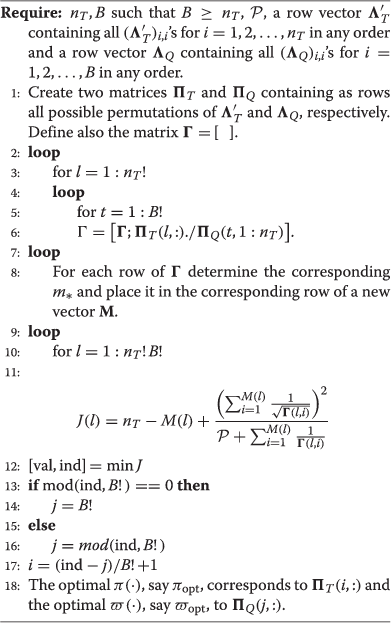
• Algorithm 1 Optimal ordering for the eigenvalues of R T ′ and S Q ′ , when R _R =S _R and ${\mathbf{R}}_T^{-1}={\mathcal{I}}_T$

  

• Note that given the fact that n _T and B are small in practice, the complexity of the above algorithm and its necessary memory are not crucial. However, as n _T and B increase, complexity and memory become important. In this case, a good solution may be to order the eigenvalues of R T′ in decreasing order and those of S Q′ in increasing order. This can be analytically justified based on the fact that for a fixed m_∗, the objective function of problem (70), say$\text{MSE}({\gamma }_1,\dots ,{\gamma }_{m_{\ast }})$, has negative partial derivatives with respect to γ _i , n i = 1, 2, …, m_∗, and it is also symmetric, since any permutation of its arguments does not change its value. This essentially shows that a good solution may maintain as active γ’s the largest possible, through the selection of m_∗. Additionally, the structure of$\text{MSE}({\gamma }_1,\dots ,{\gamma }_{m_{\ast }})$ reveals the fact that for every new active γ, something less than 1 is added to the MSE, while an inactive value corresponds to adding 1 to the MSE. This is intuitively appealing with the spatial diversity of MIMO systems and the usual properties that optimal training matrices possess in such systems (i.e., that they tend to fully exploit the available spatial diversity). The largest possible γ’s can be achieved with a decreasing order of the eigenvalues of R T′ and an increasing order of the eigenvalues of S Q′. In this case, it can be checked that m_∗ can be found as follows:

  $$\begin{array}{l}{m}_{\ast }=max\left\{m\in \{1,2,\dots ,n_T\}:\sqrt{\frac{1}{{\gamma }_m}}·\right.\\ \left.\sum _{i=1}^m\sqrt{\frac{1}{{\gamma }_i}}-\sum _{i=1}^m\frac{1}{{\gamma }_i}<\mathcal{P}\right\}.\end{array}$$

• If the modal matrices of R _R and S _R are the same,${\mathcal{I}}_T=\mathbf{I}$ and${\mathcal{I}}_R=\mathbf{I}$, then the optimal training is given by [9], as these assumptions correspond to the problem solved therein.

• In any other case (e.g., if R _R  ≠ S _R ), the (optimal) training can be found using numerical methods like the semidefinite relaxation approach described in [28]. Note that this approach can handle also general ${\mathcal{I}}_{\text{adm}}$, not necessarily Kronecker-structured.

References

Tarokh V, Naguib A, Seshadri N, Calderbank AR: Space-time codes for high data rate wireless communication: performance criteria in the presence of channel estimation errors, mobility, and multiple paths. IEEE Trans. Commun 1999, 47(2):199-207. 10.1109/26.752125
Stoica P, Besson O: Training sequence design for frequency offset and frequency-selective channel estimation. IEEE Trans. Commun 2003, 51(11):1910-1917. 10.1109/TCOMM.2003.819199
Hassibi B, Hochwald B: How much training is needed in multiple-antenna wireless links? IEEE Trans. Inf. Theory 2003, 49(4):951-963. 10.1109/TIT.2003.809594
Kotecha J, Sayeed A: Transmit signal design for optimal estimation of correlated MIMO channels. IEEE Trans. Signal Process 2004, 52(2):546-557. 10.1109/TSP.2003.821104
Wong T, Park B: Training sequence optimization in MIMO systems with colored interference. IEEE Trans. Commun 2004, 52(11):1939-1947. 10.1109/TCOMM.2004.836558
Biguesh M, Gershman A: Training-based MIMO channel estimation: a study of estimator tradeoffs and optimal training signals. IEEE Trans Signal Process 2006, 54(3):884-893.
Liu Y, Wong T, Hager W: Training signal design for estimation of correlated MIMO channels with colored interference. IEEE Trans Signal Process 2007, 55(4):1486-1497.
Katselis D, Kofidis E, Theodoridis S: Training-based estimation of correlated MIMO fading channels in the presence of colored interference. Signal Process 2007, 87(9):2177-2187. 10.1016/j.sigpro.2007.02.016
Björnson E, Ottersten B: A framework for training-based estimation in arbitrarily correlated Rician MIMO channels with Rician disturbance. IEEE Trans. Signal Process 2010., 58(3):
Biguesh M, Gazor S, Shariat M: Optimal training sequence for MIMO, wireless systems in colored environments. IEEE Trans. Signal Process 2009, 57(8):3144-3153.
Vikalo H, Hassibi B, Hochwald B, Kailath T: On the capacity of frequency- selective channels in training-based transmission schemes. IEEE Trans. Signal Process 2004, 52(9):2572-2583. 10.1109/TSP.2004.832020
Ahmed K, Tepedelenlioglu C, Spanias A: PEP-based optimal training for MIMO systems in wireless channels. Proc. IEEE ICASSP 2005, 3: 793-796.
Jansson H, Hjalmarsson H: Input design via LMIs admitting frequency-wise model specifications in confidence regions. IEEE Trans Aut. Control 2005, 50(10):1534-1549.
Bombois X, Scorletti G, Gevers M, Van den, Hof P M J, Hildebrand R: Least costly identification experiment for control. Automatica 2006, 42(10):1651-1662. 10.1016/j.automatica.2006.05.016
Hjalmarsson H: System identification of complex and structured systems. Plenary address European Control Conference/European Journal of Control 2009, 15(4):275-310.
Kiefer J: General equivalence theory for optimum designs (approximate theory). Ann. Stat 1974, 2(5):849-879. 10.1214/aos/1176342810
Ciblat P, Bianchi P, Ghogho M: Training sequence optimization for joint channel and frequency offset estimation. IEEE Trans. Signal Process 2008, 56(8):3424-3436.
Kermoal J, Schumacher L, Pedersen K, Mogensen P, Fredriksen F: A stochastic MIMO radio channel model with experimental validation. IEEE J. Sel. Areas Commun 2002, 20(6):1211-1226. 10.1109/JSAC.2002.801223
Yu K, Bengtsson M, Ottersten B, McNamara D, Karlsson P, Beach M: Modeling of wideband MIMO radio channels based on NLOS indoor measurements. IEEE Trans. Veh. Technol 2004, 53(3):655-665. 10.1109/TVT.2004.827164
Gazor S, Rad H: Space-time frequency characterization of MIMO, wireless channels. IEEE Trans. Wireless Commun 2006, 5(9):2369-2376.
Rad H, Gazor S: The impact of non-isotropic scattering and directional antennas on MIMO multicarrier mobile communication channels. IEEE Trans. Commun 2008, 56(4):642-652.
Werner K, Jansson M: Estimating MIMO channel covariances from training data under the Kronecker model. Signal Process 2009, 89: 1-13. 10.1016/j.sigpro.2008.06.014
Kay S: Fundamentals of Statistical Signal Processing: Estimation Theory. Englewood Cliffs, New Jersey: Prentice-Hall; 1993.
Rojas CR, Agüero JC, Welsh JS, Goodwin GC: On the equivalence of least costly and traditional experiment design for control. Automatica 2008, 44(11):2706-2715. 10.1016/j.automatica.2008.03.023
Barenthin M, Hjalmarsson H: Identication and control: joint input design and H∞ state feedback with ellipsoidal parametric uncertainty via LMIs. Automatica 2008, 44(2):543-551. 10.1016/j.automatica.2007.06.025
Bombois X, Hjalmarsson H: Optimal input design for robust H2, deconvolution filtering. In 15th IFAC Symposium on System Identification, Saint-Malo, July 2009. (IEEE, Piscataway); 2009.
Rojas CR, Katselis D, Hjalmarsson H, Hildebrand R, Bengtsson M: Chance constrained input design. In Proceedings of CDC-ECC, Orlando,December 2011. IEEE, Piscataway; 2011.
Katselis D, Rojas CR, Hjalmarsson H, Bengtsson M: Application-oriented finite sample experiment design: a semidefinite relaxation approach. In SYSID 2012, Brussels, July 2012. IEEE, Piscataway; 2012.
Gerencsér L, Hjalmarsson H, Mårtensson J: Adaptive input design for ARX systems. In European Control Conference, Kos, July 2007. Piscataway: IEEE; 2007.
Paulraj A, Nabar R, Gore D: Introduction to Space-Time Wireless Communications. Cambridge: Cambridge University Press; 2003.
Verdú S: Multiuser Detection. Cambridge: Cambridge University Press; 1998.
Haykin S: Adaptive Filter Theory. Englewood Cliffs: Prentice-Hall; 2001.
Hochwald B, Peel CB, Swindlehurst AL: A vector-perturbation technique for near-capacity multiantenna multiuser communication—part I: channel inversion and regularization. IEEE Trans. Commun 2005, 53: 195-202. 10.1109/TCOMM.2004.840638
Marshall AW, Olkin I New York: Academic Press; 1979.
Ostrowski A: A quantitative formulation of Sylvester’s law of inertia, II. Proc. Nat. Acad. Sci. USA 1960, 46(6):859-862. 10.1073/pnas.46.6.859
Author information
Authors and Affiliations
Corresponding author
Additional information
Competing interests
The authors declare that they have no competing interests.
Authors’ original submitted files for images
Below are the links to the authors’ original submitted files for images.
Rights and permissions
Open Access This article is distributed under the terms of the Creative Commons Attribution 2.0 International License (https://creativecommons.org/licenses/by/2.0), which permits unrestricted use, distribution, and reproduction in any medium, provided the original work is properly cited.
About this article
Cite this article
Katselis, D., Rojas, C.R., Bengtsson, M. et al. Training sequence design for MIMO channels: an application-oriented approach. J Wireless Com Network 2013, 245 (2013). https://doi.org/10.1186/1687-1499-2013-245
Received:
Accepted:
Published:
DOI: https://doi.org/10.1186/1687-1499-2013-245