Hello scheme for vehicular ad hoc networks: analysis and design

Abstract

In vehicular ad hoc networks (VANETs), essentially the information of one-hop neighbors is important for data delivery. In a general way, each node broadcasts short packets, i.e., hello packets, to indicate its appearance and establishes a neighbor table for storing neighbor information through receiving others’ hello packets. As a popular approach, it is named as a hello scheme. Determining the validity of the neighbor table, a hello scheme is vital to routing protocols in VANETs. However, a hello scheme with high accuracy and low overhead is severely challenged due to the highly dynamic topology and restricted vehicle mobility in VANETs. To address the issue, it is crucial to optimally configure two key parameters, called as hello interval (HI) and timeout interval (TI), respectively. In this article, a probability model of the hello scheme for VANETs is proposed. It is used to analyze factors affecting the two key parameters. Depending on derivation results, an effective local information-based adaptive hello scheme (LAH) is proposed subsequently. It utilizes the local information, i.e., the variation of neighbor table and received hello packets, to adjust HI and TI adaptively. According to different TI adjustment algorithms, four variants of LAH are designed as LAH-I, LAH-L, LAH-1, and LAH-2. In the end, a comparison between LAH schemes and existing three solutions is conducted to evaluate the performance. Results verify that the proposed LAH schemes are capable of obtaining higher accuracy of neighbor table and lower overhead.

1. Introduction

Vehicular ad hoc networks (VANETs) have fascinated researchers in recent years [1]. In such a network, each node maintains a table, called neighbor table, to record the information of its one-hop neighbors. Then the routing decision at each node primarily depends on messages in the table. The data dissemination of a node may be inefficient if the node omits a neighbor in its neighbor table. If a pseudo neighbor is listed in the table, forwarding decision may be false. Therefore, the accuracy of the neighbor table is a key factor for the performance of routing protocols in VANETs.

The neighbor table is achieved, thanks to the hello scheme in which each node exchanges short packets, i.e., hello packets to advertise its presence. Meanwhile, every node receives hello packets to build and update its neighbor table [2]. In general, a hello scheme includes three parts. The first part is hello delivery. Each node in the network broadcasts a hello packet every hello interval (HI). When a node receives a new hello packet, it will set up or update the relevant neighbor’s entry in its neighbor table according to the information in the packet. This is the second part. The last one is the neighbor table maintenance. In this part, a node will delete a neighbor’s entry in its table if it does not receive a new hello over a period of time, called timeout interval (TI), from the neighbor [3]. Therefore, HI and TI are determinants of the accuracy of the neighbor table and the performance of routing protocols in VANETs. However, they are difficult to configure due to their influence on network overhead.

In most existing works, the periodic hello scheme [4] is regularly utilized. Because of the fixed two intervals, its overhead is constant while the accuracy of the neighbor table is dropping quickly with the increasing node speed. Consequently, it is not suitable for high mobility networks, such as VANETs. In GPSR [5], HI of a node is jittered by 50%, i.e., the mean inter-hello transmission interval is HI _i , uniformly distributed in [0.5HI _i , 1.5HI _i . It is not effective to improve neighbor table accuracy though the hello packet collision between different nodes can be reduced. Then an improved method is presented, in which a node emits a hello packet every S meters of the distance it moves [6]. But only local mobility is considered. To estimate the two parameters from the global perspective, an adaptive scheme called TAP [7] adjusts HI according to the variation of the neighbor table unboundedly. However, all of the above schemes do not discuss the lifetime of neighbors in the neighbor table. Afterwards the neighbor lifetime algorithm (NAL) is presented [8]. It changes TI adaptively based on the history of HI. Nonetheless, different from traditional mobile ad hoc networks [9, 10], VANET is a special mobile ad hoc network for its features, such as the restricted vehicle mobility and highly dynamic. Performances of all the above hello schemes need to be tested in VANETs.

In this article, first, a probability model of the hello scheme in VANETs is proposed. Based on the model, three theorems are proposed. First of all, HI has a logical relationship with the variation of the neighbor table which is handy information. However, HI has maximum and minimum thresholds in VANETs due to the features of the network mobility. The last one is that the value of TI can be more appropriate by special information in hello packets of VANETs. Depending on derivation results, an effective local information-based adaptive hello scheme (LAH) is proposed. It utilizes local information, i.e., the variation of the neighbor table and messages in hello packets, to adjust HI and TI adaptively. According to different TI adjustment algorithms, four variants of LAH are designed as LAH-I, LAH-L, LAH-1, and LAH-2. In the end, a comparison between LAH schemes and current three solutions is conducted in one dual carriageway scenario of VANETs. Simulation results show that the proposed LAH schemes outperform existing solutions in terms of neighbor table accuracy and scheme overhead. To the best of the authors’ knowledge, this is the first effort for the comprehensive research on hello schemes in vehicular communication scenarios. In short, the contributions of this study are listed as follows.

• 1. A probability model for hello scheme in VANETs is proposed which is used to analyze factors affecting two heart parameters of a hello scheme, i.e., TI and HI.

• 2. Effective hello schemes for VANETs are proposed in the article, which can satisfy requirements of VANETs by adjusting HI and TI adaptively. It can exquisitely handle the tradeoff between the accuracy of a hello scheme and the scheme overhead.

• 3. Three available hello schemes and the proposed LAH schemes are implemented on simulation platform in this article. To evaluate the performance of a hello scheme, three specific metrics are put forward for the first time. Then a comprehensive performance evaluation is conducted through simulation results.

The remainder of the article is structured as follows. Section 2 describes the probability model for the hello scheme in VANETs. The main idea of LAH is presented in Section 3. In Section 4, evaluation results are revealed through simulations. Finally, Section 5 concludes and prospects this article.

2. Analytical model

An isotropic probability model for a hello scheme in mobile wireless networks is presented [11]. However, the model cannot be accepted in VANETs because nodes (or vehicles) have restrictions on moving. Therefore, we design a new probability model for the hello scheme in VANETs.

As shown in Figure 1, a single carriageway is selected as the research object since it is a basic module of a map. Comparing with the road width, the transmission range of a node is much larger. Thus, we assume that the carriageway is a straight line with length L. The vehicle arrive process follows a Poisson distribution that is an excellent model for vehicle arrival rate. Its intensity is λ > 0. All nodes have the same transmission range R and direction of movement. A node will not change its direction due to the restriction of the road. Node i has a velocity which magnitude is v _i , and its HI and TI are described by variables HI _i and TI _i , respectively.

Figure 1

View of the model.

Without loss of generality, considering a random node A, we assume that it is static and establish a coordinate system with A as the origin, shown in Figure 1. Any other node, like node B, has a relative speed to the reference node A, which magnitude is v _AB = |v _A – v _B | and the direction is related to v _A – v _B . A couple of variables (Time, Coordinate) are used to indicate the time and position state of a node, which means the location of the node is Coordinate at the moment of Time. T_in and T_out describe moments that node B moves into and out of the transmission range of node A, respectively, when v _AB ≠ 0. Thus, if the relative speed orientation of node B is consistent with the coordinate axis, i.e., v _A < v _B , node B has a state (T_in,–R) when it moves into the range of A. In addition, it has a state (T_out, R) when it drives away. Conversely, node B has states (T_in, R) and (T_out, –R) if the relative speed is in the opposite direction of coordinate axis, i.e., v _A > v _B . Then we have

$$T_{\mathrm{\text{out}}}=T_{\mathrm{in}}+\frac{2R}{v_{\mathit{AB}}}$$

(1)

We assume that the state of B is (T, x) when A broadcasts the k th hello packet at the moment of T. It is known that when A sends the (k + t) th hello packet B has (T + t HI _A , x _t ), in which

$$\begin{array}{l}{x}_t=x\pm v_{\mathit{AB}}\cdot t{\mathrm{HI}}_A,\\ t=-k,-k+1\cdots -1,0,1,2,3\cdots \end{array}$$

(2)

In addition, T _j describes that the time B sends the j th hello packet when B is moving inside the transmission range of A. At this time, B has a coordinate x _Bj , the state is (T _j , x _Bj ), and

$$T_{j+1}=T_j+{\mathrm{HI}}_B,j=1,2,3\cdots \frac{T_{\mathrm{\text{out}}}-T_1}{{\mathrm{HI}}_B}$$

(3)

A random variable D is introduced to denote the time interval from the entrance of B to the transmission area of A until the next hello of A is issued. Similarly, the random variable S indicates the period of time from the entrance of B to the transmission area of node A until the next hello of B is issued. Thus, we know

$$T_1=T_{\mathrm{in}}+S$$

(4)

The probability distribution function (pdf) of D and S is given by the Palm calculus [12, 13] as

$$f_D\left(D\right)=\frac{1}{E\left[{\mathrm{HI}}_A\right]}\left(1-F_{{\mathrm{HI}}_A}\left(D\right)\right)$$

(5)

and

$$f_S\left(S\right)=\frac{1}{E\left[{\mathrm{HI}}_B\right]}\left(1-F_{{\mathrm{HI}}_B}\left(S\right)\right)$$

(6)

where E[HI _B and E[HI _A are the average HI of B and A, respectively, and $F_{{\mathrm{HI}}_B}\left(*\right)$ and $F_{{\mathrm{HI}}_A}\left(*\right)$ are the distribution of the HI of B and A, respectively. The two nodes have same distribution and average of HI because nodes A and B utilize the same hello scheme. Thus, S and D have the same pdf, cumulative distribution function (cdf) and range. Then, we can obtain the cdf of the random variable S – D, depicted as F_S-D(⋅), which is useful in the following analysis.

Inspired by Ingelrest et al. [7], we realize that the variation of a neighbor table, location, velocity, and direction is the local information which is easily measured. If we are able to discover the relationship between these information and the heart parameters of hello scheme, i.e., HI and TI, we can improve the performance of hello scheme depending on the information. There are three suppositions about the hello scheme in VANETs. In the following, we will try to demonstrate them one-by-one. Definition of symbols utilized in this articleis listed in Table 1, and nodes A and B represent the reference node and a random node, respectively.

Table 1 Symbols

Theorem 1

We define that the variation of a neighbor table is the ratio between the number of new neighbors during a HI and the current total number of neighbors at the end of the HI, remarked as r. Then r is equal to N_new/N_cur, in which N_new describes the number of new neighbors during the HI and N_cur is the current total number of neighbors at the end of the HI. It is found that values of r and the HI have a real-time corresponding relationship, i.e., the expression of r is an increasing function of HI.

Proof

To verify the viewpoint, we try to get the expression of r, namely given a HI of A we must get N_new and N_cur. Without loss of generality, a HI of node A from T to T + HI _A is selected to study. This theorem is focus on HI, thus an ideal TI algorithm is adopted, i.e., node A will delete the entry of B in its neighbor table once B moves away from the range of it.

• 1. Value of N _new

  First of all, we calculate the value of N_new. The probability of a random node B that can be a new neighbor of node A during the given HI is denoted as p_new. Once p_new is known, N_new is simply equal to

  $$N_{\mathrm{\text{new}}}=\mathit{\lambda L}{p}_{\mathrm{\text{new}}}$$

  (7)

  Considering the value of p_new, there are two cases. In case one, node B is outside of the transmission range of node A at T, as shown in Figure 2. The probability of the event that node B can be a new neighbor of node A can be obtained by

  $$\begin{array}{l}{p}_1=\mathrm{Pr}\left\{B\mathrm{is}\mathrm{\text{out}}\mathrm{\text{side}}\mathrm{\text{range}}\mathrm{of}A\mathrm{at}T\right\}\\ \mathrm{Pr}\left\{B\mathrm{\text{lies}}\mathrm{in}\mathrm{\text{range}}\mathrm{of}A\mathrm{at}T+{\mathrm{HI}}_{\mathrm{A}}\right\}\\ \times \mathrm{Pr}\left\{B\mathrm{\text{sends}}\mathrm{at}\mathrm{\text{least}}\mathrm{a}\mathrm{\text{hello}}\mathrm{\text{during}}\left[T_{\mathrm{in}},T+{\mathrm{HI}}_A\right]\right\}\end{array}$$

  (8)

  Figure 2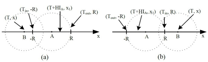

  

  Case 1. (a)v _A < v _B . (b)v _A > v _B .

  According to the relative velocity between B and A (shown in Figure 2a,b), the value of p₁ is

  $$\begin{array}{l}{p}_1=\mathrm{Pr}\left\{v_A<v_B\right\}\mathrm{Pr}\left\{x<-R\right\}\\ \mathrm{Pr}\left\{-R<x+v_{\mathit{AB}}{\mathrm{HI}}_A<R\right\}\\ \mathrm{Pr}\left\{S<D\right\}+\mathrm{Pr}\left\{v_A>v_B\right\}\\ P\left\{x>R\right\}\mathrm{Pr}\left\{-R<x-v_{\mathit{AB}}{\mathrm{HI}}_A<R\right\}\\ \mathrm{Pr}\left\{S<D\right\}=\frac{1}{2}\\ (\mathrm{Pr}\left\{-R-v_{\mathit{AB}}{\mathrm{HI}}_A<x<\min \left\{-R,R-v_{\mathit{AB}}{\mathrm{HI}}_A\right\}\right\}\\ \mathrm{Pr}\left\{S-D<0\right\}\\ +\mathrm{Pr}\left\{\mathrm{\text{max}}\left\{-R+v_{\mathit{AB}}{\mathrm{HI}}_A,R\right\}<x<R+v_{\mathit{AB}}{\mathrm{HI}}_A\right\}\\ \mathrm{Pr}\left\{S-D<0\right\})\end{array}$$

  (9)

  We define p₀ = P{v _AB HI _A > 2R}, then

  $$\begin{array}{l}{p}_1=\frac{\left(1-p_0\right)}{2}(\mathrm{Pr}\left\{-R-v_{\mathit{AB}}{\mathrm{HI}}_A<x<-R\right\}\\ \mathrm{Pr}\left\{S-D<0\right\}+\mathrm{Pr}\left\{R<x<R+v_{\mathit{AB}}{\mathrm{HI}}_A\right\}\\ \mathrm{Pr}\left\{S-D<0\right\})\\ +\frac{p_0}{2}(\mathrm{Pr}\left\{-R-v_{\mathit{AB}}{\mathrm{HI}}_A<x<R-v_{\mathit{AB}}{\mathrm{HI}}_A\right\}\hfill \\ \mathrm{Pr}\left\{S-D<0\right\}\\ +\mathrm{Pr}\left\{-R+v_{\mathit{AB}}{\mathrm{HI}}_A<x<R+v_{\mathit{AB}}{\mathrm{HI}}_A\right\}\hfill \\ \mathrm{Pr}\left\{S-D<0\right\})=\left(1-p_0\right)\frac{v_{\mathit{AB}}{\mathrm{HI}}_A}{L}{F}_{S-D}\left(0\right)\\ +p_0\frac{2R}{L}{F}_{S-D}\left(0\right)\end{array}$$

  (10)

  In VANETs, the transmission range of a node varies from 100 to 300 m while the velocity of a vehicle is less than 35 m/s. Therefore, it is a small probability event that p₀ is bigger than zero. We can ignore p₀ in most cases, especially in dense scenarios. Then we have

  $$p_1\approx \left(1-p_0\right)\frac{v_{\mathit{AB}}{\mathrm{HI}}_A}{L}{F}_{S-D}\left(0\right)\approx \frac{v_{\mathit{AB}}{\mathrm{HI}}_A}{L}{F}_{S-D}\left(0\right)$$

  (11)

  In case 2, node B lies in the transmission range of A at the time of T, as shown in Figure 3. The probability that node B can be a new neighbor of node A can be calculated from

  $$\begin{array}{l}{p}_2=\mathrm{Pr}\left\{B\mathrm{is}\mathrm{\text{inside}}\mathrm{\text{range}}\mathrm{of}A\mathrm{\text{from}}T\mathrm{to}T+{\mathrm{HI}}_A\right\}\hfill \\ \times \mathrm{Pr}\left\{B\mathrm{\text{broadcasts}}0\mathrm{\text{hello}}\mathrm{\text{packet}}\mathrm{\text{during}}\left[T_{\mathrm{in}},T\right]\right\}\hfill \\ \times \mathrm{Pr}\left\{B\mathrm{\text{sends}}\mathrm{at}\mathrm{\text{least}}\mathrm{a}\mathrm{\text{hello}}\mathrm{\text{during}}\left[T,T+{\mathrm{HI}}_A\right]\right\}\hfill \\ =\mathrm{Pr}\left\{v_A<v_B\right\}\mathrm{Pr}\left\{-R<x<R\right\}\hfill \\ \mathrm{Pr}\left\{-R<x+v_{\mathit{AB}}{\mathrm{HI}}_A<R\right\}{\displaystyle {\sum }_{k=0}^{N-1}}\hfill \\ \mathrm{Pr}\left\{D+k{\mathrm{HI}}_A<S<D+\left(k+1\right){\mathrm{HI}}_A\right\}\hfill \\ +\mathrm{Pr}\left\{v_A>v_B\right\}\mathrm{Pr}\left\{-R<x<R\right\}\hfill \\ \mathrm{Pr}\left\{-R<x-v_{\mathit{AB}}{\mathrm{HI}}_A<R\right\}{\displaystyle {\sum }_{k=0}^{N-1}}\hfill \\ \mathrm{Pr}\left\{D+k{\mathrm{HI}}_A<S<D+\left(k+1\right){\mathrm{HI}}_A\right\}\hfill \\ =\frac{2R-v_{\mathit{AB}}{\mathrm{HI}}_A}{L}{\displaystyle {\sum }_{k=0}^{N-1}\left(F_{S-D}\left(\left(k+1\right){\mathrm{HI}}_A\right)-F_{S-D}\left(k{\mathrm{HI}}_A\right)\right)}\hfill \\ =\frac{2R-v_{\mathit{AB}}{\mathrm{HI}}_A}{L}\left(F_{S-D}\left(N\cdot {\mathrm{HI}}_A\right)-F_{S-D}\left(0\right)\right),\hfill \end{array}$$

  (12)

  in which $N=\mathrm{\text{min}}\left(⌊\frac{T_{\mathrm{\text{out}}}-T_{\mathrm{in}}-D}{{\mathrm{HI}}_A}⌋\right.,\left.⌈\frac{\left|S-D\right|}{{\mathrm{HI}}_A}⌉\right).$

  Figure 3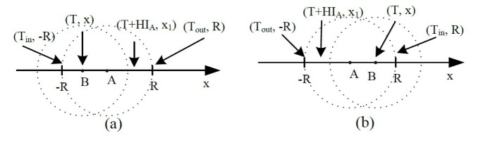

  

  Case 2. (a)v _A < v _B . (b)v _A > v _B .

  Then p_new is given by

  $$p_{\text{new}}=p_1+p_2.$$

  (13)

  Utilizing Equation(7), we have

  $$\begin{array}{l}{N}_{\mathrm{\text{new}}}=\mathit{\lambda L}{p}_{\mathrm{\text{new}}}=\lambda \left(v_{\mathit{AB}}{\mathrm{HI}}_A{F}_{S-D}\left(0\right)+\left(2R-v_{\mathit{AB}}{\mathrm{HI}}_A\right)\right.\\ \left.\left(F_{S-D}\left(N\cdot {\mathrm{HI}}_A\right)-F_{S-D}\left(0\right)\right)\right)\hfill \end{array}$$

  (14)

• 2. Value of N _cur

  To calculate the value of N_cur, we must get the probability of a random node B that can be a neighbor of node A at T + HI _A (regard the probability as p_cur). As with calculation of p_new, both cases are needed to be considered. Then we have

  $$\begin{array}{l}{p}_1\text{'}=\mathrm{Pr}\left\{B\mathrm{is}\mathrm{\text{out}}\mathrm{\text{side}}\mathrm{of}\mathrm{\text{range}}\mathrm{of}A\mathrm{at}T\right\}\hfill \\ \mathrm{Pr}\left\{B\mathrm{\text{lies}}\mathrm{in}\mathrm{\text{range}}\mathrm{of}A\mathrm{at}T+{\mathrm{HI}}_A\right\}\hfill \\ \times \mathrm{Pr}\left\{B\mathrm{\text{sends}}\mathrm{at}\mathrm{\text{least}}\mathrm{a}\mathrm{\text{hello}}\mathrm{\text{during}}\left[T_{\mathrm{in}},T+{\mathrm{HI}}_A\right]\right\}\hfill \\ =\frac{v_{\mathit{AB}}{\mathrm{HI}}_A}{L}{F}_{S-D}\left(0\right)\hfill \end{array}$$

  (15)
  $$\begin{array}{l}{p}_2\text{'}=\mathrm{Pr}\left\{B\mathrm{is}\mathrm{\text{inside}}\mathrm{of}\mathrm{\text{range}}\mathrm{of}A\mathrm{\text{from}}T\mathrm{to}T+{\mathrm{HI}}_A\right\}\hfill \\ \times \mathrm{Pr}\left\{B\mathrm{\text{sends}}\mathrm{at}\mathrm{\text{least}}\mathrm{a}\mathrm{\text{hello}}\mathrm{\text{during}}\left[T_{\mathrm{in}},T+{\mathrm{HI}}_A\right]\right\}\hfill \\ =\mathrm{Pr}\left\{v_A<v_B\right\}\mathrm{Pr}\left\{-R<x<R\right\}\hfill \\ \mathrm{Pr}\left\{-R<x+v_{\mathit{AB}}{\mathrm{HI}}_A<R\right\}{\displaystyle \sum }_{k=0}^{N-1}\hfill \\ \mathrm{Pr}\left\{S<D+\left(k+1\right){\mathrm{HI}}_A\right\}+\mathrm{Pr}\left\{v_A>v_B\right\}\hfill \\ \mathrm{Pr}\left\{-R<x<R\right\}\mathrm{Pr}\left\{-R<x-v_{\mathit{AB}}{\mathrm{HI}}_A<R\right\}{\displaystyle \sum }_{k=0}^{N-1}\hfill \\ \mathrm{Pr}\left\{S<D+\left(k+1\right){\mathrm{HI}}_A\right\}\hfill \\ =\frac{2R-v_{\mathit{AB}}{\mathrm{HI}}_A}{L}{\displaystyle {\sum }_{k=1}^N{F}_{S-D}\left(k\cdot {\mathrm{HI}}_A\right)}\hfill \end{array}$$

  (16)

  and

  $$p_{\mathrm{\text{cur}}}=p_1\text{'}+p_2\text{'}$$

  (17)

  Therefore

  $$N_{\mathrm{\text{cur}}}=\mathit{\lambda L}{p}_{\mathrm{\text{cur}}}=\lambda \left(v_{\mathit{AB}}{\mathrm{HI}}_A{F}_{S-D}\left(0\right)+\left(2R-v_{\mathit{AB}}{\mathrm{HI}}_A\right){\displaystyle {\sum }_{k=1}^N{F}_{S-D}\left(k\cdot {\mathrm{HI}}_A\right)}\right).$$

  (18)

• 3. Value of r

  Then the variation of the neighbor table of A is given by

  $$r=\frac{N_{\mathrm{\text{new}}}}{N_{\mathrm{\text{cur}}}}=\frac{v_{\mathit{AB}}{\mathrm{HI}}_A{F}_{S-D}\left(0\right)+\left(2R-v_{\mathit{AB}}{\mathrm{HI}}_A\right)\left(F_{S-D}\left(N\cdot {\mathrm{HI}}_A\right)-F_{S-D}\left(0\right)\right)}{v_{\mathit{AB}}{\mathrm{HI}}_A{F}_{S-D}\left(0\right)+\left(2R-v_{\mathit{AB}}{\mathrm{HI}}_A\right){{\displaystyle \sum }}_{k=1}^N{F}_{S-D}\left(k\cdot {\mathrm{HI}}_A\right)})$$

  (19)

  N > 1 is a small probability event because S – D has a range [-HI, HI]. In order to simplify the calculation, we ignore the case of N > 1. Then calculating the derivative with respect to HI _A , we have

  $$\frac{\mathit{dr}}{d{\mathrm{HI}}_A}|N=1=\frac{2R{v}_{\mathit{AB}}{F}_{S-D}{}^2\left(0\right)+{\left(2R-v_{\mathit{AB}}{\mathrm{HI}}_A\right)}^2{F}_{S-D}\left(0\right)\frac{d{F}_{S-D}\left({\mathrm{HI}}_A\right)}{d{\mathrm{HI}}_A}}{{\left(v_{\mathit{AB}}{\mathrm{HI}}_A{F}_{S-D}\left(0\right)+\left(2R-v_{\mathit{AB}}{\mathrm{HI}}_A\right)F_{S-D}\left({\mathrm{HI}}_A\right)\right)}^2}>0$$

  (20)

  namely the expression of r is an increasing function of HI _A and Theorem 1 is demonstrated. At the same time, some useful conclusions are derived as follows.

  • a. Factors impacting HI are the variation of neighbor table, node transmission range, and relative speed between nodes.

  • b. The neighbor table variation responses to the change of HI, that is consistent with the idea in [7].

  • c. The number of new neighbor in the neighbor table grows, namely r increases, if node A sends hello slowly. At this time, node A must generate more hello packets to announce the new coming neighbors of its presence. Thus, it should reduce HI _A . On the contrary, r is reduced with the decreasing HI _A . Then the number of new neighbors diminishes and node A does not broadcast so many hello packets with high overhead. In this condition, the value of HI _A must be increased. Utilizing the logical relationship, the value of HI _A can easily be decided. It demonstrates the theory that it can adjust HI based on the variation of neighbor table in VANETs.

Theorem 2

HI has minimum and maximum thresholds in VANETs.

Proof

To calculate Equation(19) with respect to v _AB , we have

$$\frac{\mathit{dr}}{d{v}_{\mathit{AB}}}|N=1=\frac{2R{\mathrm{HI}}_A{F}_{S-D}{}^2\left(0\right)}{{\left(v_{\mathit{AB}}{\mathrm{HI}}_A{F}_{S-D}\left(0\right)+\left(2R-v_{\mathit{AB}}{\mathrm{HI}}_A\right)F_{S-D}\left({\mathrm{HI}}_A\right)\right)}^2}>0.$$

(21)

It means that the variation of the neighbor table rises with the increasing node velocity. However, velocity of a vehicle in VANETs is affected by the speed limit of road, the vehicle in front, and the network density. When the network density is sparse, speed of a vehicle can reach the maximum speed limit of the road. Then with the increasing network density, the maximum speed reached by a vehicle is smaller than maximum speed limit of the road once the network is saturated. So, a random vehicle in VANETs has a maximum velocity. Thus, HI has a minimum threshold while the variation of the neighbor table has a maximum value.

At the same time, hello packets in VANETs carry node information as position, velocity, and direction. To ensure the propagation of the information, HI must have a maximum threshold.

Theorem 3

The value of TI can be more appropriate utilizing information in hello packets.

Proof

A node deletes a neighbor’s entry in its table if it does not receive a new hello of the neighbor over a period of time. This period of time is TI. The most appropriate value of TI is equal to the time a neighbor move away from the transmission range of the node. As shown in Figure 4, node B moves into the transmission range of A at T_in. Then node B broadcasts the j th hello packet at T _j since it moves into the transmission area of A. B departs from the transmission range of A at T_out. Therefore, the proper time that node A delete the entry of B is

$$\begin{array}{l}{\mathrm{TI}}_B=T_{\mathrm{out}}-T_j=\left(T_{\mathrm{in}}+\frac{2R}{v_{\mathit{AB}}}\right)-\left(T_{\mathrm{in}}+S+j{\mathrm{HI}}_B\right)\\ =\frac{2R}{v_{\mathit{AB}}}-S-j{\mathrm{HI}}_B.\end{array}$$

(22)

Figure 4

Analysis of TI. (a)AtT_in. (b)AtT _j . (c)AtT_out.

However, in traditional ad hoc networks, the fixed TI is usually adopted instead of the appropriate one because the appropriate value is hard to be obtained. Xue et al. [14]proposed that VANETs are well behaved and can predict accurately. Hello packets in VANETs have information as location, speed, and direction. Thus, by the method of prediction, the value of TI can be more accurate. Then TI of B in neighbor table of A is

$${\mathrm{TI}}_{{}_B}=\{\begin{array}{cc}\hfill \frac{R-x_{\mathit{Bj}}}{v_{\mathit{AB}}}\hfill & \hfill v_A>v_B\hfill \\ \hfill \frac{R+x_{\mathit{Bj}}}{v_{\mathit{AB}}}\hfill & \hfill v_A<v_B\hfill \end{array}$$

(23)

Particularly, the interval is infinite in theory if the relative velocity of nodes A and B is equal to 0. Nonetheless, the value can be set up for some special purpose.

According to the above analysis, we have some conclusions. First, HI has logical relationships with the variation of neighbor table, depicted as Equation(19). HI has thresholds because of the move features of nodes in VANETs. The last one is that TI can be more accurate by the position prediction algorithm. Depending on the derivation results, we design our hello schemes in Section 3.

3. The proposed protocol

Depending on the above analysis, a novel adaptive scheme for VANETs, called LAH, is proposed. LAH is a rounded hello scheme, in which HI and TI are changed adaptively according to the information in the neighbor table. In LAH, a node first regulates its HI and broadcasts a hello packet. It waits until the HI expired. Then a new hello packet is generated and sent. Meanwhile, every node in the networks receives hello packets from other nodes for building its neighbor table and calculating TI. A node will delete an entry of a neighbor in its table if it does not receive a new hello from the neighbor until TI expired. The details of HI adjustment algorithm and TI adjustment algorithm are as follows.

3.1. HI adjustment algorithm

A node will calculate its parameter r each time it broadcasts a hello packet. Then HI is adjusted based on r. For this a node should deposit two up-to-date neighbor tables. For instance, there are two neighbor tables, Table _n and Table_n+1, in Figure 5. Comparing them, nodes E and F are determined as new neighbors. In this case, r is equal to 2 divided by 4.

Figure 5

Neighbor differentiation.

Depending on the conclusion in Section 2, that the value of r reflects that whether HI fits for the current network scenario, we can build a relationship expression for adjusting HI, as

$$\begin{array}{lll}\mathrm{HI}=\left\{\begin{array}{cc}\hfill {\mathrm{HI}}_{\text{min}}\hfill & \hfill {\mathrm{HI}}^{\prime }<{\mathrm{HI}}_{\text{min}}\hfill \\ \hfill {\mathrm{HI}}_{\text{max}}\hfill & \hfill {\mathrm{HI}}^{\prime }>{\mathrm{HI}}_{\text{max}}\hfill \\ \hfill {\mathrm{HI}}^{\prime }\hfill & \hfill \mathrm{\text{otherwise}}\hfill \end{array}\right.& ,\hfill & \mathrm{\text{where}}\hfill \\ {\mathrm{HI}}^{\text{'}}=\left\{\begin{array}{cc}\hfill \mathrm{HI}+\frac{\mathrm{HI}}{\alpha }\hfill & \hfill r\le r_{\mathrm{th}}\hfill \\ \hfill \mathrm{HI}-\frac{\mathrm{HI}}{\beta }\hfill & \mathrm{\text{otherwise}}\hfill \end{array}\right.& ,\hfill \end{array}$$

(24)

where α, β, and r_th are the adjustment factors, HI_min and HI_max are thresholds of HI. The five parameters are empirical value, which can be set manually on the basis of network conditions. However, any other functions satisfying the relationship can be utilized.

3.2. TI adjustment algorithm

Depending on the difference of information in hello packets, there are four TI algorithms. Thus, LAH has four variants.

• a. LAH-L

  If there are location and velocity in hello, a node (as node A) receives a hello packet from a neighbor (depicted as B) and it calculates TI of B according to Equation(24). If A does not receive a new hello from B during TI, it will delete the entry of B in its neighbor table. This time our scheme is called LAH-L.

• b. LAH-I

  If the ideal position prediction algorithm is adopted, the LAH is the perfect one, named LAH-I. In the situation, node A will delete the entry of B in its neighbor table once B moves away from the range of it.

• c. LAH-1 and LAH-2

  However, not all hello packets have location and velocity information. In this case, the simple and effective method is that nodes change TI of one neighbor with the neighbor’s up-to-data HI, that is

  $${\mathrm{TI}}_B=n{\mathrm{HI}}_B$$

  (25)

in which the integer n is the number of allowable hello loss. n = 1 means that all hello packets can be received correctly, remarked as LAH-1 otherwise it has hello loss. If n = 2, the scheme is described as LAH-2.

4. Simulation results

In this section, we evaluate the performance of seven hello schemes, which are the existing three schemes, namely periodic, TAP, and NAL, and our schemes. For different TI adjustment methods, our schemes have different names. LAH-I has ideal position prediction arithmetic while LAH-L utilizes the current speed and location to predict the next moment. LAH-1 and LAH-2 depict the regulation of TI depending on Equation(25) with n = 1 and n = 2, respectively.

4.1. Simulation scenarios

Performance of LAH, TAP, and NAL is evaluated with NS-2 [15], which is the most popular network simulator in academia because of its open-source and plenty of components library. A realistic mobility model called Intelligent Driver Model with Lane Changes (IDM-LC) [16] is utilized in our simulation. IDM-LC is a time-continuous car-following model with the characteristics of car overtaking and intersection management. As shown in Figure 6, there are 100 nodes randomly distributed in a 4-lane road, and the length of the road is L = 3 km.The desired speed of the nodes changed from 10 to 100 km/h. The IEEE 802.11 distributed coordinating function is used as medium access control sublayer protocol for all nodes in the simulation. The radio transmission range for each node is 150 m. And the initialization settings of these schemes are

• 1. In periodic hello scheme, each node generates a hello packet every 1 s and TI is 2 s.

• 2. The initial HI of TAP is 1 s. For the absence of TI algorithm in TAP, we use 2HI as the value of TI in simulation of TAP.

• 3. NAL is a scheme without HI adjustment algorithm. Thus, NAL is coupled with TAP.

• 4. All LAH schemes have the same initial HI that is 1 s. The initial value of TI is 2 s.

Figure 6

Mobility model of the scenario.

4.2. Performance metrics

To measure the performance of the neighbor table, four metrics are designed in this article, which are validity, reliability, general accuracy, and overhead. For a random node (as node A), m denotes the number of all the actual neighbors of A, k expresses the number of valid neighbors in its neighbor table, and l describes the current total number of neighbors in the node’s table.

Validity is defined as k/m. It is in direct proportion to the number of the valid neighbors, because the number of the actual neighbors is constant. A small HI and a high TI contribute to the increase of the valid neighbors, which will improve the validity. When a hello scheme is used in a routing protocol, the validity can show the probability that the selected next-hop is the best one.

Reliability is denoted by k/l. It shows the difference between the total number of nodes and the number of actual neighbors in the neighbor table. The reliability will get higher with the decreasing HI and increasing TI. When a hello scheme is utilized in a routing protocol, the reliability can describe the probability that the selected node is a right next-hop.

General accuracy is equal to k/(m + l – k), which can generally illuminate the accuracy of the neighbor table. Both HI and TI have influence on it.

Overhead is average number of hello packets that a node sends in the simulation.

For example, the neighbor relationship of a node A is shown in Figure 7. In fact there are seven neighbors in the radio propagation range of A. None of the blue nodes can directly communicate with A. Due to missing and lag of hello packets, there are six neighbors recorded in table of A. It includes five valid neighbors and a false node D, while actual neighbors B and C are missing. Therefore, the validity, reliability, and general accuracy, respectively, are 5/7, 5/6, and 5/(7 + 6 – 5).

Figure 7

Neighbor relationship.

4.3. Results and analysis

The following four figures show our simulation results, which are accuracy of neighbor table and overhead of hello packets. The accuracy results are shown in Figures 8, 9, and 10. The accuracy of the periodic hello scheme decreases quickly with the increasing node speed. However, the adaptive scheme, namely TAP, NAL, and LAH, falls slowly. It demonstrates that the adaptive hello scheme works better than the periodic scheme in high dynamic networks. Unlike the simulation results in [7, 8], the accuracy of TAP and NAL is worse than the periodic in low mobility scenarios. The reason is that HI and TI are 1 and 2 s, respectively, which is very small but not necessary value of the two intervals in low mobility scenarios. However, the two intervals are set as 3 and 6 s in [7, 8]. Figure 11 depicts the overhead of hello scheme, namely the number of hello packets during the simulation process. Comparing accuracy results with overhead, we get that the adaptive scheme hasan acceptable accuracy with low overhead while the periodic scheme keep similar accuracy with higher overhead in low mobility scenarios. However, in high mobility scenarios the adaptive one keep high accuracy with compromising overhead. Thus, the adaptive hello scheme is more suitable for dynamic networks, as VANETs.

Figure 8

Validity.

Figure 9

Reliability.

Figure 10

General accuracy.

Figure 11

Overhead.

The validity results of all the above seven schemes are shown in Figure 8. The validity is equal to the ratio between the number of valid node in the neighbor table and realistic neighbor. It depends on the number of valid node in the neighbor table because the number of realistic neighbor is fixed. HI has a crucial role in the number of valid node. Therefore, the shorter HI is, the higher the validity of the hello scheme has. Indeed, TI has a weak influence on the validity because it will delete valid node in the neighbor table by too short TI and the validity will be decreased. In Figure 8, TAP and NAL have the same HI adjustment algorithm. Thus, they have similar validity. For the constant small HI, namely a hello per second, the validity of periodic scheme is better than TAP and NAL in low mobility scenarios. Our hello schemes have a much higher validity, i.e., about 2% higher than TAP and NAL. In low mobility scenarios, the validity of LAH is similar with the periodic while it is about 2.5% higher than the periodic. It clarifies that the HI adjustment algorithm of LAH is better availability than the existing schemes in terms of validity.

Figure 8 also compares several LAH schemes. Among them, LAH-I adopts ideal position prediction algorithm, i.e., in its neighbor table any valid node does not disappear and any redundancy node does not appear. Therefore, LAH-I has perfect validity among our schemes. The curve of LAH-2 is closest to LAH-I in Figure 8. The reason is that LAH-2 has a large TI and it will not remove a valid neighbor. For the small value of TI, LAH-2 has a low validity. Furthermore, LAH-L has the lowest performance for the same reason. Viewed from this angle, an ideal position prediction algorithm is helpful for a high validity adaptive hello scheme.

Figure 9 depicts the reliability of all the schemes, which is impressed by both the HI and TI algorithm. Theoretically, the reliability of LAH-I is 100% by adopting the ideal position prediction algorithm. However, there are some redundancy nodes in the neighbor table for the random statistics time, which result in ups and downs in the reliability curve of LAH-I. The reliability of LAH-L is similar with LAH-1, and about 2% higher than LAH-2. It follows that if TI is twice of HI, the redundancy nodes in the neighbor table are much more, and then the reliability will be reduced. In low mobility scenarios, the reliability of LAH-2 is about 2% larger than NAL. However, LAH-2 has no superiority in high mobility scenarios. It verifies that adaptive TI algorithm is more suitable for high dynamic networks.

The general accuracy of the neighbor table is described in Figure 10, which simply reflects the accuracy of the neighbor table. From the figure, we can get that LAH-I has the best performance in the term of accuracy, whereas the performance of LAH-L adopting the simple position prediction algorithm is lower than LAH-1 and higher than LAH-2. Compared with NAL, LAH-2 has nearly 3% improvements. The results verify LAH-I can keep the accuracy of neighbor table in VANET. However, it needs an exact position prediction algorithm. The sub-optimal scheme LAH-1 is unrealistic for its too small TI. This is because there are many other packets filled in VANETs, as data packets. Thus, the hello packet has high lost for the collision between packets. With the too small TI LAH-1 will expurgate valid neighbors. Then the performance of routing decision will be decreased. In general, with appropriate location prediction algorithm LAH-L can achieve high performance, which is much suitable for VANETs.

Figure 11 describes the overhead, the total hello packets broadcasted by all nodes in the network. The curves of all adaptive schemes are increasing with node speed. The reason is that they need more hello packets to keep the neighbor table up-to-date at a higher node speed. The overhead of periodic hello scheme is fixed for the constant two intervals. Thus, periodic has low accuracy in high mobility scenarios. TAP has the lowest overhead. At the same time it has the lowest accuracy, revealed from Figures 8, 9, and 10. All LAH schemes have similar overhead because they utilize the same HI adjustment algorithm. NAL has lower accuracy than LAH though it has lower overhead in slow-speed scenarios. Then in high mobility scenarios, the overhead of NAL increases quickly. Nevertheless, the accuracy of LAH is still higher than NAL. It means that compared with the current three schemes, LAH works better on compromising between accuracy of the neighbor table and overhead of hello scheme in VANETs.

5. Conclusions

A hello scheme is critical for routing decision in VANETs. However, settling into a neat balance between the accuracy of neighbor table and the scheme overhead it is complicated by the fact that VANETs are highly dynamic and mobility restricted. To address this problem, we proposed a probability model to analyze factors affecting two vital parameters of a hello scheme, namely HI and TI. Based on the model, three theorems are demonstrated. Then effective LAH is proposed depending on derivation results. It utilizes local information, i.e., the variation of the neighbor table and messages in hello packets, to adjust HI and TI adaptively. According to different TI adjustment algorithms, four variants of LAH are designed as LAH-I, LAH-L, LAH-1, and LAH-2. Experimental results show that the general accuracy of the proposed LAH schemes is about 3% higher than existing solutions while the overhead of LAH is at least 20% lower than current adaptive schemes. Among the proposed LAH schemes, LAH-I has much better performance though it needs high-precision position prediction algorithm.

As future work, we will modify the probability model in more complex VANET scenarios and design precise location prediction algorithm to improve the performance of LAH schemes. If possible we also want to analyze how much does the accuracy of neighbor table influence routing protocols.

References

Mohamed W: Advances in Vehicular Ad-hoc Networks: Developments and Challenges. Information Science Reference, USA; 2010:149-170.
Hernandez-Cons N, Kasahara S, Takahashi Y: Dynamic hello/timeout timer adjustment in routing protocols for reducing overhead in MANETs. Comput. Commun. 2010, 33(15):1864-1878. 10.1016/j.comcom.2010.06.011
Alsaqour R, Abdelhaq M, Alsukour O: Effect of network parameters on neighbor wireless link breaks in GPSR protocol and enhancement using mobility prediction model. EURASIP J. Wirel. Commun 2012. 10.1186/1687-1499-2012-171
Moy J: Open shortest path first(ospf) version 2, RFC 2178. http://www.rfc-editor.org/rfc/rfc2178.txt
Karp B, Kung H: GPSR: greedy perimeter stateless routing for wireless networks,Proceedings of the Sixth Annual International Conference on Mobile Computing and Networking (MobiCom). Boston, August; 2000:243-254.
Griuka V, Singhal M: Hello protocols for ad-hoc networks: overhead and accuracy tradeoffs,Proceedings of World of Wireless Mobile and Multimedia Networks (WoWMoM 2005). Taormina, June; 2005:354-361.
Ingelrest F, Mitton N, Simplot-Ryl D: A turnover based adaptive hello protocol for mobile ad hoc and sensor networks,Proceedings of 15th International Symposium on Modeling, Analysis, and Simulation of Computer and Telecommunication Systems (MASCOTS '07). Istanbul, October; 9-14.
Ahmad-Kassem A, Mitten N: Adapting dynamically neighbourhood table entry lifetime in wireless sensor networks,Proceedings of International Conference on Wireless Communications & Signal Processing (WCSP 2010). China, October; 2010:1-6.
Wang X, Huang W, Wang S, Zhang J, Hu C: Delay and capacity tradeoff analysis for motioncast. IEEE ACM Trans. Netw. 2011, 19(5):1354-1367.
Wang X, Fu L, Hu C: Multicast performance with hierarchical cooperation. IEEE ACM Trans. Netw. 2012, 20(3):917-930.
Heissenbüttel M, Braun T, Wälchli M, Bernoulli T: Evaluating the limitations of and alternatives in beaconing. Ad Hoc Netw. 2007, 5(5):558-578. 10.1016/j.adhoc.2006.03.002
Nayebi A, Karlsson G, Sarbazi-Azad H: Evaluation and design of beaconing in mobile wireless networks. Ad Hoc Netw. 2011, 9(3):368-386. 10.1016/j.adhoc.2010.08.014
Heyman DP, Sobel MJ: Stochastic Models in Operations Research,1st edn. McGraw-Hill, New York; 1982.
Xue G, Luo Y, Yu J, Li M: A novel vehicular location prediction based on mobility patterns for routing in urban VANET. EURASIP J. Wirel. Commun 2012. 10.1186/1687-1499-2012-222
NS-2, Network Simulator tool. http://www.isi.edu/nsnam/ns/
Trieber M, Hennecke A, Helbing D: Congested traffic states in empirical observations and microscopic simulations. Phys. Rev. 2000, E62(2):1805-1824.
Acknowledgments
This study was supported by the National Natural Science Foundation of China under Grant no. 61271176, the National Science and Technology Major Project under Grant no. 2011ZX03001-007-01 and 2013ZX03004007-003, the Special Research Fund of State Key Laboratory under Grant no. ISN1102003, the Open Research Fund of National Mobile Communications Research Laboratory, Southeast University under Grant no. 2012D01, and the 111 Project (B08038).
Author information
Authors and Affiliations
Corresponding author
Additional information
Competing interests
The authors declare that they have no competing interests.
Authors’ original submitted files for images
Below are the links to the authors’ original submitted files for images.
Rights and permissions
Open Access This article is distributed under the terms of the Creative Commons Attribution 2.0 International License (https://creativecommons.org/licenses/by/2.0), which permits unrestricted use, distribution, and reproduction in any medium, provided the original work is properly cited.
About this article
Cite this article
Li, C., Zhu, L., Zhao, C. et al. Hello scheme for vehicular ad hoc networks: analysis and design. J Wireless Com Network 2013, 28 (2013). https://doi.org/10.1186/1687-1499-2013-28
Received:
Accepted:
Published:
DOI: https://doi.org/10.1186/1687-1499-2013-28