Capacity analysis of LTE-Advanced HetNets with reduced power subframes and range expansion

Abstract

The use of reduced power subframes in LTE Rel. 11 can improve the capacity of heterogeneous networks (HetNets) while also providing interference coordination to the picocell-edge users. However, in order to obtain maximum benefits from the reduced power subframes, setting the key system parameters, such as the amount of power reduction, carries critical importance. Using stochastic geometry, this paper lays down a theoretical foundation for the performance evaluation of HetNets with reduced power subframes and range expansion bias. The analytic expressions for average capacity and 5th percentile throughput are derived as a function of transmit powers, node densities, and interference coordination parameters in a two-tier HetNet scenario and are validated through Monte Carlo simulations. Joint optimization of range expansion bias, power reduction factor, scheduling thresholds, and duty cycle of reduced power subframes is performed to study the trade-offs between aggregate capacity of a cell and fairness among the users. To validate our analysis, we also compare the stochastic geometry-based theoretical results with the real macro base station (MBS) deployment (in the city of London) and the hexagonal grid model. Our analysis shows that with optimum parameter settings, the LTE Rel. 11 with reduced power subframes can provide substantially better performance than the LTE Rel. 10 with almost blank subframes, in terms of both aggregate capacity and fairness.

1 Introduction

Cellular networks are witnessing an exponentially increasing data traffic from mobile users. Heterogeneous networks (HetNets) offer a promising way of meeting these demands. They are composed of small-sized cells such as micro-, pico-, and femtocells overlaid on the existing macrocells to increase the frequency reuse and capacity of the network. Since the base stations (BSs) of different tiers use different transmission powers and typically a frequency reuse factor of 1, analyzing and mitigating the interference at an arbitrary user equipment (UE) is a challenging task.

1.1 Related work on evaluation methodology

Different approaches have been used in the literature for the performance evaluation of HetNets. The traditional simulation models with BSs placed on a hexagonal grid are highly idealized and may typically require complex and time-consuming system-level simulations. On the other hand, models based on stochastic geometry and spatial point processes provide a tractable and computationally efficient alternative for performance evaluation of HetNets [1–4]. Poisson point process (PPP)-based models have been recently used extensively in the literature for performance evaluation of HetNets. However, as the macro base station (MBS) locations are carefully planned during the deployment process, PPP-based models may not be viable for capturing real MBS locations, due to some points of the process being very close to each other. The Matern hardcore point process (HCPP) provides a more accurate alternative spatial model for MBS locations. In HCPPs, the distance between any two points of the process is greater than a minimum distance predefined by the hard core parameter. HCPP models are relatively more complicated due to the non-existence of the probability generating functional [1]. Also, HCPP has a flaw of underestimating the intensity of the points that can coexist for a given hard core parameter [5]. Hence, HCPP models are not as tractable and simple as the PPP models.

With PPPs, using simplifying assumptions, such as Rayleigh fading channel model, and a path-loss exponent of 4, we can obtain closed form expressions for aggregate interference and outage probability. Therefore, use of PPP models for performance evaluation of HetNets is appealing due to their simplicity and tractability [6]. Furthermore, the PPP-based models provide reasonably close performance results when compared with the real BS deployments. In particular, results in [3] show that, when compared with real BS deployments, PPP- and hexagonal grid-based models for BS locations provide a lower bound and an upper bound, respectively, on the outage probabilities of UEs. Also, the PPP-based models are expected to provide a better fit for analyzing denser HetNet deployments due to higher degree of randomness in small-cell deployments [2]. In this paper, due to their simplicity and reasonable accuracy, we will use PPP-based models to characterize and understand the behavior of HetNets in terms of various design parameters.

1.2 Use of PPP-based models for LTE-Advanced HetNet performance evaluation

The existing literature has numerous papers based on the PPP model for analyzing HetNets. Using PPPs, the basic performance indicators such as coverage probability and average rate of a UE are analyzed in [7–10]. The use of range expansion bias (REB) in the picocell enables it to associate with more UEs and thereby improves the offloading of UEs to the picocells. The effect of REB on the coverage probability is studied in [11, 12]. However, with range expansion, the offloaded UEs at the edge of picocells experience high interference from the macrocell. This necessitates a coordination mechanism between the MBSs and pico base stations (PBSs) to protect the picocell-edge UEs from the MBS interference. While [2, 3, 13] consider a homogeneous cellular network, [12] considers a HetNet with range expansion. The authors of [2, 3, 12] have obtained the information of real BS locations in an urban area from a cellular service provider. On the other hand, the authors of [13] have obtained the BS location information from an open source project [14] that provides approximate locations of the BSs around the world.

To mitigate the interference problems in HetNets, different enhanced inter-cell interference coordination (eICIC) techniques have been specified in LTE Rel. 10 of 3GPP which includes time-domain, frequency-domain, and power control techniques [15]. In the time-domain eICIC technique, MBS transmissions are muted during certain subframes and no data is transmitted to macro UEs (MUEs). The picocell-edge users are served by PBS during these subframes (coordinated subframes), thereby protecting the picocell-edge users from MBS interference. The eICIC technique using REB is studied well in the literature by analyzing its effects on the rate coverage [16, 17] and on the average per-user capacity [18, 19]. However, in the simulations of [20], the MBS transmits at reduced power (instead of muting the MBS completely) during the coordinated subframes (CSFs) to serve only its nearby UEs. Therein, the use of reduced power subframes during CSFs is shown to improve the HetNet performance considerably in terms of the trade-off between the cell-edge and average throughputs. Later on, reduced power subframe transmission has also been standardized under LTE Rel. 11 of 3GPP and commonly referred therein as further-enhanced ICIC (FeICIC). In another study [21], simulation results show that the FeICIC is less sensitive to the duty cycle of CSFs than the eICIC. In [22], 3GPP simulations are used to study and compare the eICIC and FeICIC techniques for different REBs and almost blank subframe densities. Therein, the amount of power reduction in the reduced power subframes is made equivalent to REB and its optimality is not justified.

1.3 Contributions

In the authors’ earlier work [7], analytic expressions for coverage probability of an arbitrary UE are derived using PPPs. Later, the analytical framework in [7] has been extended to spectral efficiency (SE) derivations in [18, 19] by considering eICIC and range expansion. Reduced power subframes, which are standardized in LTE Rel. 11 [23], are not analytically studied in the literature to our best knowledge.

In the present work, generalized SE expressions are derived considering the FeICIC which includes eICIC and no eICIC as the two special cases. In this analytic framework that uses reduced power subframes and range expansion, expressions for the average SE of UEs and the 5th percentile throughput are derived. These expressions are validated through Monte Carlo simulations. Details of the simulation model are documented explicitly, and the MATLAB codes can be accessed through [24] for regenerating the results. The optimization of key system parameters is analyzed with a perspective of maximizing both aggregate capacity in a cell and the proportional fairness among its users. Using these results, insights are developed on the configuration of FeICIC parameters, such as the power reduction level, range expansion bias, duty cycle of CSFs, and scheduling thresholds. The 5th and 50th percentile capacities are also analyzed to determine the trade-offs associated with FeICIC parameter adaptation. Further, we compare the 5th percentile SE results from the PPP model with the real MBS deployment [25] and the hexagonal grid model.

2 System model

We consider a two-tier HetNet system with MBS, PBS, and UE locations modeled as two-dimensional homogeneous PPPs of intensities λ, λ^′, and λ_u, respectively. Both the MBSs and the PBSs share a common transmission bandwidth. We assume round robin scheduling in all the downlinks of a cell. For analytical tractability, we also assume that during a subframe, a BS allocates an entire system bandwidth to a single UE. We also assume that the cells have full buffer traffic and the thermal noise is negligible when compared to interference. The MBSs employ reduced power subframes, in which they transmit at reduced power levels to prevent high interference to the picocell UEs (PUEs). On the other hand, the PBSs transmit at full power during all the subframes.

The frame structure with reduced power subframes is shown in Figure 1. During uncoordinated subframes (USFs), the MBS transmits data and control signals at full power P_tx, and during CSFs, it transmits at a reduced power α P_tx, where 0≤α≤1 is the power reduction factor. The PBS transmits the data, control signals, and cell reference symbol with power $P_{\text{tx}}^{\prime }$ during all the subframes. Setting α= 0 corresponds to eICIC, and α= 1 corresponds to the no eICIC case. A list of all the notations and symbols used in this paper are described in Table 1.

Figure 1

Frame structure with reduced power subframes, transmitted with a duty cycle of β = 0.5 .

Table 1 Notations and symbols

Define β as the duty cycle of USFs, i.e., ratio of the number of USFs to the total number of subframes in a frame. Then, (1-β) is the duty cycle of CSF/reduced power subframes. Let K and K^′ be the factors that account for geometrical parameters such as the transmitter and receiver antenna heights of the MBS and the PBS, respectively. Then, the effective transmitted power of MBS during USFs is P = P_txK, MBS during CSFs is α P, and PBS during USF/CSF is $P^{\prime }=P_{\text{tx}}^{\prime }{K}^{\prime }$. For an arbitrary UE, let the nearest MBS at a distance r be its macrocell of interest (MOI) and the nearest PBS at a distance r^′ be its picocell of interest (POI). Then, assuming Rayleigh fading channel, the reference symbol received power from the MOI and the POI are given by

$$S\left(r\right)=\frac{\mathit{\text{PH}}}{r^{\delta }},S^{\prime }\left(r^{\prime }\right)=\frac{P^{\prime }{H}^{\prime }}{{\left(r^{\prime }\right)}^{\delta }},$$

(1)

respectively, where δ is the path-loss exponent, and the random variables H∼Exp(1) and H^′∼Exp(1) account for Rayleigh fading. Define an interference term, Z, as the total interference power at a UE during USFs from all the MBSs and the PBSs, excluding the MOI and the POI. Similarly, define Z^′ as the total interference power during CSFs. We assume that there is no frame synchronization across the MBSs, and therefore irrespective of whether the MOI is transmitting a USF or a CSF, the interference at UE has the same distribution in both cases and is independent of both S(r) and S^′(r^′). Then, an arbitrary UE experiences the following four SIRs:

$$\Gamma =\frac{S\left(r\right)}{S^{\prime }\left(r^{\prime }\right)+Z},\to \text{USF SIR from MOI}$$

(2)

$${\Gamma }^{\prime }=\frac{S^{\prime }\left(r^{\prime }\right)}{S\left(r\right)+Z},\to \text{USF SIR from POI}$$

(3)

$${\Gamma }_{\text{csf}}=\frac{\mathrm{\alpha S}\left(r\right)}{S^{\prime }\left(r^{\prime }\right)+Z},\to \text{CSF SIR from MOI}$$

(4)

$${\Gamma }_{\text{csf}}^{\prime }=\frac{S^{\prime }\left(r^{\prime }\right)}{\mathrm{\alpha S}\left(r\right)+Z}.\to \text{CSF SIR from POI}$$

(5)

2.1 UE association

In (4) and (5), it can be noted that Γ_csf and ${\Gamma }_{\text{csf}}^{\prime }$ are directly affected by α, and hence, their usage will make the cell selection process dependent on α. Thus, we consider Γ and Γ^′ to minimize the dependence of the cell selection process on α.

The cell selection process using Γ, Γ^′, and the REB τ can be explained with reference to Figure 2. If τ Γ^′ is less than Γ, then the UE is associated with the MOI, otherwise with the POI. After the cell selection, the UE is scheduled either in USF or in CSF based on the scheduling thresholds ρ (for MUE) and ρ^′ (for PUE). In a macrocell, if Γ is less than ρ then the UE is scheduled to USF, otherwise to CSF. Similarly, in a picocell, if Γ^′ is greater than ρ^′ then the UE is scheduled to USF, otherwise to CSF (to protect it from macrocell interference). The cell selection and scheduling conditions can be combined and formulated as follows:

Figure 2

Illustration of UE association criteria.

$$\text{If}\Gamma >\tau {\Gamma }^{\prime }\text{and}\Gamma \le \rho \to \text{USF-MUE},$$

(6)

$$\text{If}\Gamma >\tau {\Gamma }^{\prime }\text{and}\Gamma >\rho \to \text{CSF-MUE},$$

(7)

$$\text{If}\Gamma \le \tau {\Gamma }^{\prime }\text{and}{\Gamma }^{\prime }>{\rho }^{\prime }\to \text{USF-PUE},$$

(8)

$$\text{If}\Gamma \le \tau {\Gamma }^{\prime }\text{and}{\Gamma }^{\prime }\le {\rho }^{\prime }\to \text{CSF-PUE}.$$

(9)

A sample layout of MBSs and PBSs with their coverage areas for the four different UE categories is illustrated in Figure 3. Note that in the related work of [16], the UE association criteria are based on the average reference symbol received power at UE, where as our model is based on the SIR at UE, it also encompasses the FeICIC mechanism. In [16], the boundary between the USF-PUEs (picocell area) and the CSF-PUEs (range expanded area) is fixed due to the fixed transmit power of PBS. On the other hand, in our approach, the boundary between USF and CSF users can be controlled using ρ in the macrocell and ρ^′ in the picocell, the parameters which play an important role during optimization as will be shown in Section 5.3.

Figure 3

Illustration of two-tier HetNet layout. In picocells, the coverage regions for USF- and CSF-PUEs are colored in orange and green, respectively, whereas in macrocells, the coverage regions for USF- and CSF-MUEs are colored in white and blue, respectively.

Using (1) to (5), it can be shown that the two SIRs Γ_csf and ${\Gamma }_{\text{csf}}^{\prime }$ could be expressed in terms of Γ and Γ^′ as

$${\Gamma }_{\text{csf}}=\mathrm{\alpha \Gamma },{\Gamma }_{\text{csf}}^{\prime }=\frac{{\Gamma }^{\prime }\left(1+\Gamma \right)}{1+\Gamma \left[\alpha \left({\Gamma }^{\prime }+1\right)-{\Gamma }^{\prime }\right]}.$$

(10)

Hence, knowing the statistics of Γ and Γ^′, particularly their joint probability density function (JPDF), would provide a complete picture of the SIR statistics of the HetNet system. We first derive an expression for joint complementary cumulative distribution function (JCCDF) of Γ and Γ^′ in Section 3.1. Then, we differentiate the JCCDF with respect to γ and γ^′ to get the expression for JPDF in Section 3.2, which will then be used for spectral efficiency analysis.

3 Derivation of joint SIR distribution

3.1 JCCDF of Γ and Γ^′

From (1), we know that S(r) and S^′(r^′) are exponentially distributed with mean P/r^δ and P^′/(r^′)^δ, respectively. For brevity, substitute S(r) = X and S^′(r^′) = Y in (2) and (3):

$$\Gamma =\frac{X}{Y+Z},{\Gamma }^{\prime }=\frac{Y}{X+Z}.$$

(11)

Using (11), it can be easily shown that the product Γ Γ^′ has a maximum value of 1.

Let, R and R^′ be the random variables denoting the distances of MOI and POI from a UE. Then, the JCCDF of Γ and Γ^′ conditioned on R = r,R^′ = r^′ is given by

$$\begin{array}{l}\mathbb{P}\left\{\Gamma >\gamma ,{\Gamma }^{\prime }>{\gamma }^{\prime }\left|R=r,R^{\prime }=r^{\prime }\right.\right\}\\ ={\mathbb{E}}_Z\left[\mathbb{P}\left\{X>\gamma \left(Y+Z\right),Y>{\gamma }^{\prime }\left(X+Z\right)\right\}\right],\\ ={\mathbb{E}}_Z\left[{\int }_{y1}^{+\infty }{f}_Y\left(y\right){\int }_{\gamma \left(y+Z\right)}^{y/{\gamma }^{\prime }-Z}{f}_X\left(x\right)\mathrm{d}x\mathrm{d}y\right],\end{array}$$

(12)

for γ>0, γ^′>0, and γ γ^′<1. Here, $f_{\mathrm{X}}\left(x\right)=\frac{r^{\delta }}{P}exp\left(-\frac{r^{\delta }}{P}x\right)$, $f_{\mathrm{Y}}\left(y\right)=\frac{{\left(r^{\prime }\right)}^{\delta }}{P^{\prime }}exp\left(-\frac{{\left(r^{\prime }\right)}^{\delta }}{P^{\prime }}y\right)$, and the integration limit $y_1={\gamma }^{\prime }Z\left(\frac{1+\gamma }{1-\gamma {\gamma }^{\prime }}\right).$ The integration region of (12) is graphically represented in Figure 4. By solving the integration as shown in Appendix 1, we can obtain a closed form expression for the conditional JCCDF as

$$\begin{array}{l}\mathbb{P}\left\{\Gamma >\gamma ,{\Gamma }^{\prime }>{\gamma }^{\prime }|R=r,R^{\prime }=r^{\prime }\right\}\\ =\frac{\left(1-\gamma {\gamma }^{\prime }\right){\mathcal{ℒ}}_Z\left(\frac{1}{1-\gamma {\gamma }^{\prime }}\left(\frac{\gamma \left(1+{\gamma }^{\prime }\right)r^{\delta }}{P}+\frac{{\gamma }^{\prime }\left(1+\gamma \right){\left(r^{\prime }\right)}^{\delta }}{P^{\prime }}\right)\right)}{\left[1+\gamma \frac{P^{\prime }}{P}{\left(\frac{r}{r^{\prime }}\right)}^{\delta }\right]\left[1+{\gamma }^{\prime }\frac{P}{P^{\prime }}{\left(\frac{r^{\prime }}{r}\right)}^{\delta }\right]},\end{array}$$

(13)

Figure 4

Illustration of the integration region in the JPDF of X and Y . The shaded region indicates the integration region in order to compute the JCCDF.

for γ>0,γ^′>0, and γ γ^′<1, where ${\mathcal{ℒ}}_Z\left(s\right)$ is the Laplace transform of the total interference Z.

Expression for ${\mathcal{ℒ}}_{\mathrm{Z}}\left(s\right)$ can be derived as follows. We assume that the interfering MBSs of a UE are frame asynchronous and subframe synchronous. Essentially, we wanted to assume no synchronization at all. However, this would permit part of a subframe from an interfering transmitter to interfere with part of another subframe at the receiver, and the complications for analysis would be too much. To simplify the interference scenario, we would not account for, or model, any interference by partially overlapping subframes. In other words, if a subframe partially overlaps another subframe, it is assumed to overlap completely. This is equivalent to the 'subframe-synchronized but frame-asynchronous’ assumption.

The locations of the USFs and CSFs are uniformly randomly distributed, with a USF duty cycle of β for all the MBSs. Hence, each interfering MBS transmits USFs with probability β and CSFs with probability (1-β). Therefore, the tier of MBSs can be split into two tiers: one tier of MBSs transmitting only USFs and other transmitting only CSFs. These two tiers are independent PPPs with intensities λ β and λ(1-β). Therefore, the FeICIC scenario can be modeled using three independent PPPs as illustrated in Table 2.

Table 2 PPP parameters for USF MBSs, CSF MBSs, and PBSs

Let I_usf(r), I_csf(r), and I^′(r^′) be the interference at UE from all interfering USF-MBSs, CSF-MBSs, and PBSs. Then, the total interference is Z = I_usf(r)+I_csf(r)+I^′(r^′). Using ([26], Corollary 1), parameters in Table 2, and assuming δ= 4, we can derive the Laplace transform of Z in (13) to be

$$\begin{array}{l}{\mathcal{ℒ}}_Z\left(s\right)=exp\left\{-\mathrm{\pi \beta \lambda }\sqrt{\mathit{\text{Ps}}}\left[\frac{\pi }{2}-\stackrel{-1}{tan}\left(\frac{r^2}{\sqrt{\mathit{\text{Ps}}}}\right)\right]\right.\\ -\pi \left(1-\beta \right)\lambda \sqrt{\mathrm{\alpha Ps}}\left[\frac{\pi }{2}-\stackrel{-1}{tan}\left(\frac{r^2}{\sqrt{\mathrm{\alpha Ps}}}\right)\right]\\ \left.-\pi {\lambda }^{\prime }\sqrt{P^{\prime }s}\left[\frac{\pi }{2}-\stackrel{-1}{tan}\left(\frac{{\left(r^{\prime }\right)}^2}{\sqrt{P^{\prime }s}}\right)\right]\right\}.\end{array}$$

(14)

3.2 JPDF of Γ and Γ^′

The conditional JPDF of Γ and Γ^′

$$f_{\Gamma ,{\Gamma }^{\prime }\left|R,R^{\prime }\right.}\left(\gamma ,{\gamma }^{\prime }\left|r,r^{\prime }\right.\right)=\mathbb{P}\left\{\Gamma =\gamma ,{\Gamma }^{\prime }={\gamma }^{\prime }|R=r,R^{\prime }=r^{\prime }\right\}$$

(15)

can be derived by differentiating the JCCDF in (13) with respect to γ and γ^′. Detailed derivation of conditional probability JPDF is provided in Appendix 2. Using the theorem of conditional probability, we can write

$$f_{\Gamma ,{\Gamma }^{\prime },R,R^{\prime }}\left(\gamma ,{\gamma }^{\prime },r,r^{\prime }\right)=f_{\Gamma ,{\Gamma }^{\prime }\left|R,R^{\prime }\right.}\left(\gamma ,{\gamma }^{\prime }\left|r,r^{\prime }\right.\right)f_R\left(r\right)f_{R^{\prime }}\left(r^{\prime }\right),$$

(16)

where the PDFs of R and R^′ are $f_R\left(r\right)=2\mathrm{\pi \lambda r}{e}^{-\mathrm{\lambda \pi }{r}^2}$ and $f_{R^{\prime }}\left(r^{\prime }\right)=2\pi {\lambda }^{\prime }{r}^{\prime }{e}^{-{\lambda }^{\prime }\pi {\left(r^{\prime }\right)}^2}$, respectively. We can then express the unconditional JPDF of Γ and Γ^′ as

$$\begin{array}{l}{f}_{\Gamma ,{\Gamma }^{\prime }}\left(\gamma ,{\gamma }^{\prime }\right)={\int }_{d_{\text{min}}}^{\infty }{\int }_{d_{\text{min}}^{\prime }}^{\infty }{f}_{\Gamma ,{\Gamma }^{\prime },R,R^{\prime }}\left(\gamma ,{\gamma }^{\prime },r,r^{\prime }\right)\mathrm{d}{r}^{\prime }\mathrm{d}r\\ ={\int }_{d_{\text{min}}}^{\infty }{\int }_{d_{\text{min}}^{\prime }}^{\infty }{f}_{\Gamma ,{\Gamma }^{\prime }\left|R,R^{\prime }\right.}\left(\gamma ,{\gamma }^{\prime }\left|r,r^{\prime }\right.\right)f_R\left(r\right)f_{R^{\prime }}\left(r^{\prime }\right)\mathrm{d}{r}^{\prime }\mathrm{d}r,\end{array}$$

(17)

where we assume that a UE is served by a BS only if it satisfies the minimum distance constraints: UE should be located at distances of at least d_min from the MOI and $d_{\text{min}}^{\prime }$ from the POI.

4 Spectral efficiency analysis

In this section, the expressions for aggregate and per-user SEs for different UE categories are derived. Considering the JPDF of an arbitrary UE in (17), first, the expressions for the probabilities that the UE belongs to each category are derived. Then, these expressions are used to derive the mean number of UEs of each category in a cell. These are followed by the derivation of the aggregate SE. Then, per-user SE expressions are obtained by dividing the aggregate SE by the mean number of UEs.

4.1 MUE and PUE probabilities

Depending on the SIRs Γ and Γ^′, a UE can be one of the four types: USF-MUE, CSF-MUE, USF-PUE, or CSF-PUE. Given that the UE is located at a distance r from its MOI and r^′ from its POI, probabilities of the UE belonging to each type can be found by integrating the conditional JPDF over the regions whose boundaries are set by the cell selection conditions in (6) to (9). Based on these conditions, the integration regions for different UE categories are shown in Figure 5.

Figure 5

Illustration of the integration regions in the JPDF of Γ and Γ^′. Shaded regions indicate the integration regions to compute the probabilities of a UE belonging to different categories.

The probability that a UE is a CSF-MUE can be found by integrating the JPDF over the region R1,

$$\begin{array}{c}{P}_{\text{csf}}=\mathbb{P}\left\{\Gamma >\tau {\Gamma }^{\prime },\Gamma >\rho \right\}={\int }_{\rho }^{\infty }{\int }_0^{min\left(\frac{1}{\gamma },\frac{\gamma }{\tau }\right)}{f}_{\Gamma ,{\Gamma }^{\prime }}\left(\gamma ,{\gamma }^{\prime }\right)\mathrm{d}{\gamma }^{\prime }\mathrm{d}\mathrm{\gamma .}\end{array}$$

(18)

To form concise equations, let us define an integral function

$$G\left(g,\mathrm{R}i\right)=\int {\int }_{\mathrm{R}i}g\left(\gamma ,{\gamma }^{\prime }\right)f_{\Gamma ,{\Gamma }^{\prime }}\left(\gamma ,{\gamma }^{\prime }\right)\mathrm{d}{\gamma }^{\prime }\mathrm{d}\gamma ,$$

(19)

where g is a function of γ and γ^′, and Ri for i = 1,2,3,4 is the integration region as defined in Figure 5. Then, (18) can be written as

$$P_{\text{csf}}=\mathbb{P}\left\{\Gamma >\tau {\Gamma }^{\prime },\Gamma >\rho \right\}=G\left(1,\text{R}1\right).$$

(20)

Similarly, the conditional probabilities that a UE is a USF-MUE, USF-PUE, or CSF-PUE are respectively given as

$$P_{\text{usf}}=\mathbb{P}\left\{\Gamma >\tau {\Gamma }^{\prime },\Gamma \le \rho \right\}=G\left(1,\text{R}2\right),$$

(21)

$$P_{\text{usf}}^{\prime }=\mathbb{P}\left\{\Gamma \le \tau {\Gamma }^{\prime },{\Gamma }^{\prime }\ge {\rho }^{\prime }\right\}=G\left(1,\text{R}4\right),$$

(22)

$$P_{\text{csf}}^{\prime }=\mathbb{P}\left\{\Gamma \le \tau {\Gamma }^{\prime },{\Gamma }^{\prime }<{\rho }^{\prime }\right\}=G\left(1,\text{R}3\right).$$

(23)

4.2 Mean number of MUEs and PUEs

Since the MBS locations are generated using PPPs, the coverage areas of all the MBSs resemble a Voronoi tessellation. Consider an arbitrary Voronoi cell. Let the number of UEs in the cell be N and the number of CSF-MUEs in the cell be M. Then, M is a random variable, and the mean number of CSF-MUEs is given by

$$\begin{array}{l}{N}_{\text{csf}}=E\left[M\right]=E\left[\sum _{n=1}^{N}1\left\{\text{UE}n\text{is a CSF-MUE}\right\}\right]\\ =E_N\left\{E\left[\sum _{n=1}^{N}1\left\{\text{UE}n\text{is a CSF-MUE}\right\}\left|N\right.\right]\right\}\\ =E_N\left\{\sum _{n=1}^{N}E\left[1\left\{\text{UE}n\text{is a CSF-MUE}\right\}\right]\right\},\end{array}$$

(24)

where in (24) we use the fact that the probability that any of the N UEs in a cell being a CSF-MUE is independent of N. However, it is important to note that this is itself a consequence of our assumption that there is no limit on the number of CSF-MUEs per cell. Further, the event that any of the UEs in a cell is a CSF-MUE is independent of the event that any other UE in that cell is a CSF-MUE, and all such events have the same probability of occurrence, namely P_csf given in (20). Then,

$$N_{\text{csf}}=E_N\left\{\sum _{n=1}^N{P}_{\text{csf}}\right\}=E_N\left[N{P}_{\text{csf}}\right]=P_{\text{csf}}E\left[N\right].$$

(25)

Using ([27], Lemma 1), it can be shown that the mean number of UEs in a Voronoi cell is λ_u/λ. Therefore, the mean number of CSF-MUEs in a cell is given by

$$N_{\text{csf}}=\frac{P_{\text{csf}}{\lambda }_{\text{u}}}{\lambda }.$$

(26)

Similarly, the mean number of USF-MUEs, USF-PUEs, and CSF-PUEs is respectively given by

$$N_{\text{usf}}=\frac{P_{\text{usf}}{\lambda }_{\mathrm{u}}}{\lambda },N_{\text{usf}}^{\prime }=\frac{P_{\text{usf}}^{\prime }{\lambda }_{\mathrm{u}}}{{\lambda }^{\prime }},N_{\text{csf}}^{\prime }=\frac{P_{\text{csf}}^{\prime }{\lambda }_{\mathrm{u}}}{{\lambda }^{\prime }}.$$

(27)

4.3 Aggregate and per-user spectral efficiencies

We use Shannon capacity formula, log2(1+SIR), to find the SE of each UE type. The mean aggregate SE of an arbitrarily located CSF-MUE can be found by

$$\begin{array}{c}{C}_{\text{csf}}\left(\lambda ,{\lambda }^{\prime },\tau ,\alpha ,\rho ,\beta \right)=\left(1-\beta \right)\frac{\mathbb{E}\left[\underset{2}{log}\left(1+{\Gamma }_{\text{csf}}\right)\left|\text{UE is a CSF-MUE}\right.\right]}{P_{\text{csf}}}\\ =\left(1-\beta \right)\frac{G\left(\underset{2}{log}\left(1+{\gamma }_{\text{csf}}\right),\mathrm{R}1\right)}{P_{\text{csf}}},\\ =\left(1-\beta \right)\frac{G\left(\underset{2}{log}\left(1+\mathrm{\alpha \gamma }\right),\text{R}1\right)}{P_{\text{csf}}}.\end{array}$$

(28)

Similarly, the mean aggregate SEs for USF-MUEs, USF-PUEs, and CSF-PUEs can be respectively derived to be

$$C_{\text{usf}}\left(\lambda ,{\lambda }^{\prime },\tau ,\alpha ,\rho ,\beta \right)=\beta \frac{G\left(\underset{2}{log}\left(1+\gamma \right),\mathrm{R}2\right)}{P_{\text{usf}}},$$

(29)

$$C_{\text{usf}}^{\prime }\left(\lambda ,{\lambda }^{\prime },\tau ,\alpha ,{\rho }^{\prime },\beta \right)=\beta \frac{G\left(\underset{2}{log}\left(1+{\gamma }^{\prime }\right),\mathrm{R}4\right)}{P_{\text{usf}}^{\prime }},$$

(30)

$$C_{\text{csf}}^{\prime }\left(\lambda ,{\lambda }^{\prime },\tau ,\alpha ,{\rho }^{\prime },\beta \right)=\left(1-\beta \right)\frac{G\left(\underset{2}{log}\left(1+{\gamma }_{\text{csf}}^{\prime }\right),\mathrm{R}3\right)}{P_{\text{csf}}^{\prime }},$$

(31)

where ${\gamma }_{\text{csf}}^{\prime }=\frac{{\gamma }^{\prime }\left(1+\gamma \right)}{1+\gamma [\alpha \left({\gamma }^{\prime }+1\right)-{\gamma }^{\prime }]}$. Then, the corresponding per-user SEs are

$$C_{\text{u,usf}}\left(\lambda ,{\lambda }^{\prime },\tau ,\alpha ,\rho ,\beta \right)=\frac{\lambda C_{\text{usf}}\left(\lambda ,{\lambda }^{\prime },\tau ,\alpha ,\rho ,\beta \right)}{{\lambda }_{\mathrm{u}}{P}_{\text{usf}}},$$

(32)

$$C_{\text{u,csf}}\left(\lambda ,{\lambda }^{\prime },\tau ,\alpha ,\rho ,\beta \right)=\frac{\lambda C_{\text{csf}}\left(\lambda ,{\lambda }^{\prime },\tau ,\alpha ,\rho ,\beta \right)}{{\lambda }_{\mathrm{u}}{P}_{\text{csf}}},$$

(33)

$$C_{\text{u,usf}}^{\prime }\left(\lambda ,{\lambda }^{\prime },\tau ,\alpha ,{\rho }^{\prime },\beta \right)=\frac{{\lambda }^{\prime }{C}_{\text{usf}}^{\prime }\left(\lambda ,{\lambda }^{\prime },\tau ,\alpha ,{\rho }^{\prime },\beta \right)}{{\lambda }_{\mathrm{u}}{P}_{\text{usf}}^{\prime }},$$

(34)

$$C_{\text{u,csf}}^{\prime }\left(\lambda ,{\lambda }^{\prime },\tau ,\alpha ,{\rho }^{\prime },\beta \right)=\frac{{\lambda }^{\prime }{C}_{\text{csf}}^{\prime }\left(\lambda ,{\lambda }^{\prime },\tau ,\alpha ,{\rho }^{\prime },\beta \right)}{{\lambda }_{\mathrm{u}}{P}_{\text{csf}}^{\prime }}.$$

(35)

4.4 5th percentile throughput

The 5th percentile throughput reflects the throughput of cell-edge UEs. Typically, the cell-edge UEs experience high interference, and analyzing their throughput provides important information about the fairness among the users in a cell and the system performance.

Consider the JPDF expression in (17). The integration regions of the JPDF for different UE categories are shown in Figure 5. The SIR PDF of USF-MUEs can be evaluated by integrating the JPDF over γ^′ in region R2,

$$\begin{array}{c}{f}_{\Gamma }\left(\gamma \right)=\mathbb{P}\left\{\Gamma =\gamma \left|\text{UE is a USF-MUE}\right.\right\}\\ ={\int }_0^{min\left(\frac{\gamma }{\tau },\frac{1}{\gamma }\right)}{f}_{\Gamma ,{\Gamma }^{\prime }}\left(\gamma ,{\gamma }^{\prime }\right)\mathrm{d}{\gamma }^{\prime },\end{array}$$

(36)

for 0≤γ≤ρ. The CDF expression can be derived as

$$\begin{array}{c}{\mathrm{F}}_{\Gamma }\left({\gamma }_{\text{usf}}\right)=\mathbb{P}\left\{\Gamma \le {\gamma }_{\text{usf}}\left|\text{UE is a USF-MUE}\right.\right\}\\ ={\int }_0^{{\gamma }_{\text{usf}}}{f}_{\Gamma }\left(\gamma \right)\mathrm{d}\gamma ={\int }_0^{{\gamma }_{\text{usf}}}{\int }_0^{min\left(\frac{\gamma }{\tau },\frac{1}{\gamma }\right)}{f}_{\Gamma ,{\Gamma }^{\prime }}\left(\gamma ,{\gamma }^{\prime }\right)\mathrm{d}{\gamma }^{\prime }\mathrm{d}\gamma ,\end{array}$$

(37)

for 0 ≤γ_usf ≤ρ, and the CDF of throughput of the USF-MUEs can be derived as a function of F _Γ (γ_usf) in (37) as

$$\begin{array}{l}{\mathrm{F}}_{C_{\text{usf}}}\left(c_{\text{usf}}\right)=\mathbb{P}\left\{C_{\text{usf}}\le c_{\text{usf}}\left|\text{UE is a USF-MUE}\right.\right\}\\ =\mathbb{P}\left\{\underset{2}{log}\left(1+{\Gamma }_{\text{usf}}\right)\le c_{\text{usf}}\left|\text{UE is a USF-MUE}\right.\right\},\\ =\mathbb{P}\left\{{\Gamma }_{\text{usf}}\le \left(2^{c_{\text{usf}}}-1\right)\left|\text{UE is a USF-MUE}\right.\right\}\\ ={\mathrm{F}}_{\Gamma }\left(2^{c_{\text{usf}}}-1\right),\end{array}$$

(38)

for 0≤c_usf≤ log2(1+ρ). By using the CDF plots, the 5th percentile throughput of USF-MUEs can easily be found as the value at which the CDF is equal to 0.05. Similarly, the 5th percentile throughput of other three UE categories can also be found.

5 Numerical and simulation results

The average SE and 5th percentile throughput expressions derived in the earlier sections are validated using a Monte Carlo simulation model built in MATLAB. Validation of the PPP capacity results for a HetNet scenario with range expansion and reduced power subframes is a non-trivial task. In this section, details of the simulation approach used for validating the PPP analyses are explicitly documented to enable reproducibility. MATLAB codes for the simulation model, and the theoretical analysis can be downloaded from [24].

5.1 Simulation methodology for verifying PPP model

The algorithm used in the simulation to find the aggregate and per-user SEs is described below.

• 1. The X- and Y-coordinates of MBSs, PBSs, and UEs are generated using uniformly distributed random variables. The mean number of MBS and PBS location marks is λ A and λ ^′ A, respectively, where A is the assumed geographical area that is square in shape as illustrated in Figure 6.

  Figure 6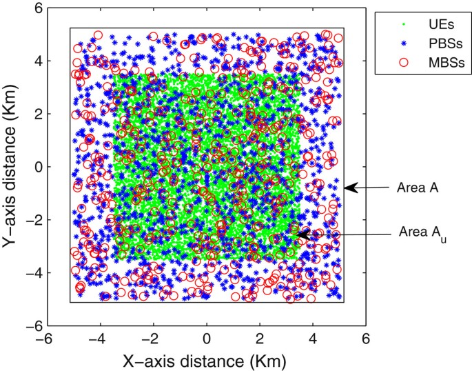

  

  Simulation layout.

• 2. In the PPP analysis, the geographical area is assumed to be infinite. In such case, it is important to account for edge effects in the simulations. In a tessellation that is defined on an unbounded region, what happens outside a bounded simulation window may effect what happens within the window [28]. As the simulation area is limited, if a UE is located at the edge of the simulation area, the BSs around it will not be symmetrically distributed. Hence, to avoid the edge effects, the UE locations are constrained within a smaller area A _u that is aligned at the center of the main simulation area A to avoid the UEs from being located at the edges. The mean number of UEs in the area A _u is λ _u A _u.

• 3. The MOI (closest MBS) and POI (closest PBS) for each UE are identified. The minimum distance constraints are applied by discarding the UEs that are closer than $d_{\text{min}}\left(d_{\text{min}}^{\prime }\right)$ from their respective MOIs (POIs).

• 4. The SIRs Γ, Γ ^′, Γ _csf, and ${\Gamma }_{\text{csf}}^{\prime }$ are calculated for each UE using (2) to (5).

• 5. The UEs are classified as USF-MUEs, CSF-MUEs, USF-PUEs, and CSF-PUEs using the conditions in (6) to (9).

• 6. The MUEs (PUEs) which share the same MOI (POI) are grouped together to form the macro- and picocells.

• 7. The SEs of all the UEs are calculated. In a cell, SE of a USF-MUE i is calculated using $\frac{\beta \underset{2}{log}\left(1+{\Gamma }_i\right)}{\left(\text{No. of USF-MUEs in the cell}\right)}$. The SEs of other UE types are calculated using similar formulations.

• 8. The aggregate capacity of each UE type is calculated in all the cells.

• 9. Mean aggregate capacity and mean number of UEs of each type are calculated by averaging over all the cells.

• 10. The per-user SE of each UE type is calculated by (mean aggregate capacity)/(mean number of UEs).

5.2 Per-user SEs with PPPs and Monte Carlo simulations

The system parameter settings are shown in Table 3. The per-user SE results obtained using the analytic expressions of (32) to (35) are compared with the simulation results in Figure 7a,b for macrocell and picocell, respectively. The averaging process in the simulations is not straightforward, and it can be explained as follows. With reference to Figure 6, the inner simulation area A_u where the UEs are distributed consists of a random number of macrocells and picocells in each simulation instance. On average, it contains λ A_u macrocells and λ^′A_u picocells. Since the simulation results are obtained by averaging over the macrocells and picocells, we can say that the simulation results were obtained by averaging over approximately λ A_uN_sim macrocells and λ^′A_uN_sim picocells, where N_sim is the number of simulation instances. Using the parameter values in Table 3 and N_sim = 20, we can say that the simulation results were obtained by averaging over approximately 4,508 macrocells and 13,524 picocells.

Table 3 Parameter settings

Figure 7

Per-user SE in (a) macrocell and (b) picocell. For the case with β = 0.5, ρ = 4 dB, and ρ^′ = 0 dB.

The analytic and simulation plots in Figure 7a,b match with sufficient accuracy. However, there exists a slight disagreement between the analytic and simulation results which could be due to the fact that the calculation of analytic results involves four nested integrals. Since the numerical integration in MATLAB has certain tolerance limits, the results could be off the ideal values. Another source for disagreement could be due to the fact that in theoretical analysis, the BSs are assumed to be distributed over an infinite geographical area. However, the simulations are performed using a finite area of 10×10 km ². Nevertheless, Figure 7 provides the following insights.

5.2.1 USF- and CSF-MUEs

Referring to Figure 2, USF-MUEs form the outer part and CSF-MUEs form the inner part of the macrocell. As the REB increases, some of the USF-MUEs at the macro-pico boundary which have worse SIRs are offloaded to the picocell. Consequently, the mean number of USF-MUEs decreases and their per-user SE increases as shown in Figure 7a.

The mean number of CSF-MUEs are not affected by τ as long as $\sqrt{\tau }\le \rho$. Considering Figure 5, it can be noted that if $\sqrt{\tau }=\rho$, the line γ=τ γ^′ intersects the boundary of region R1. Hence, if τ is increased further such that $\sqrt{\tau }>\rho$, the area of R1 decreases and thereby decreases the mean number of CSF-MUEs. Therefore, the per-user SE of CSF MUEs remains constant as long as $\sqrt{\tau }\le \rho$ and increases if τ crosses this limit as shown in Figure 7a.

On the other hand, as the α increases, the transmit power of all the interfering MBSs increases during CSFs; hence, it increases the interference power Z at all the UEs. This causes the SIRs of USF-MUEs (Γ), USF-PUEs (Γ^′), and CSF-PUEs (${\Gamma }_{\text{csf}}^{\prime }$) to decrease, which can be noted in (2), (3), and (5), respectively. However, the SIRs of CSF-MUEs (Γ_csf) would increase (despite of increased interference) because of the increase in received signal power (due to higher α) which can be noted in (4). Considering (6) and (7), since ρ is a constant, the degradation in Γ causes the number of USF-MUEs to increase and CSF-MUEs to decrease. Consequently, the per-user SE of USF-MUEs decreases and that of CSF-MUEs increases for increasing α, as shown in Figure 7a.

5.2.2 USF- and CSF-PUEs

As the REB increases, the mean number of USF-PUEs remains constant if ${\rho }^{\prime }>1/\sqrt{\tau }$ because the area of region R4 in Figure 5 is unaffected by the value of τ. Therefore, the per-user SE of USF-PUEs also remains constant for increasing REB as shown in Figure 7b. With increasing REB, some MUEs are offloaded to the picocell and become CSF-PUEs. But these UEs are located at cell-edges and have low SIRs. Hence, the per-user SE of CSF-PUEs decreases as shown in Figure 7b.

On the other hand, as the α increases, the transmit power of all the interfering MBSs increases during CSFs causing Γ, Γ^′, and ${\Gamma }_{\text{csf}}^{\prime }$ to decrease and Γ_csf to increase, as explained previously. Considering (8) and (9), since ρ^′ is a constant, the degradation in Γ^′ causes the number of USF-PUEs to decrease and CSF-PUEs to increase. Consequently, the per-user SE of USF-PUEs increases and that of CSF-PUEs decreases for increasing α, as shown in Figure 7b.

5.3 Optimization of system parameters to achieve maximum capacity and proportional fairness

The five parameters τ, α, β, ρ,andρ^′ are the key system parameters that are critical to the satisfactory performance of the HetNet system. The goal of these parameter settings is to maximize the aggregate capacity in a cell while providing proportional fairness among the users.

Consider an arbitrary cell which consists of N UEs. Let C _i be the capacity of an arbitrary UE i∈{1, 2,…, N}. The sum of capacities (sum-rate) and the sum of log capacities (log-rate) in a cell are respectively given by

$$C_{\text{sum}}=\sum _{i=1}^N{C}_i,C_{\text{log}}=\sum _{i=1}^{N}log\left(C_i\right)=log\left(\sum _{i=1}^N{C}_i\right).$$

(39)

Maximizing the C_sum corresponds to maximizing the aggregate capacity in a cell, while maximizing the C_log corresponds to proportional fair resource allocation to the users of a cell ([29], App. A) [30]. There can be trade-offs existing between aggregate capacity and fairness in a cell. Maximizing the C_sum may reduce the C_log and vice versa. In this section, we try to understand these trade-offs by analyzing the characteristics of C_log and C_sum with respect to the variation of key system parameters.

We attempt to maximize the aggregate capacity and the proportional fairness among the users by jointly optimizing the five key system parameters which can be mathematically formulated as

$$\underset{\rho ,{\rho }^{\prime },\alpha ,\tau ,\beta }{\max }{C}_{\text{sum}}=\underset{\rho ,{\rho }^{\prime },\alpha ,\tau ,\beta }{\max }\sum _{i=1}^N{C}_i,$$

(40)

and

$$\underset{\rho ,{\rho }^{\prime },\alpha ,\tau ,\beta }{\max }{C}_{\text{log}}=\underset{\rho ,{\rho }^{\prime },\alpha ,\tau ,\beta }{\max }log\left(\prod _{i=1}^N{C}_i\right).$$

(41)

We solve the optimization problem numerically with brute-force search technique. As there are five optimization parameters, this problem involves searching for an optimum solution in a five-dimensional space. The variation of C_log with respect to ρ, ρ^′, α, and τ is shown in Figure 8, for β=0.5. These plots are obtained through the Monte Carlo simulations, and each plot is the variation of C_log with respect to ρ for fixed values of ρ^′, α, and τ. The optimum scheduling thresholds ρ∗ and ρ^′∗ that maximize the C_log are dependent on the values of α and τ.

Figure 8

Sum of log capacities versus the scheduling thresholds for different α and τ combinations.

In this paper, we have used a simple brute-force search technique to optimize the system parameters, while it is also possible to use non-linear optimization techniques. For example, reinforcement learning method is used in [31, 32] to optimize the downlink transmission strategies in HetNets such as the transmit power and the REB. In [33], a game theoretic approach and distributed learning algorithm are used to optimize the downlink transmit power, REB, and the ON/OFF states of individual BSs to minimize the system cost which includes energy and load expenditures. Typically, these optimization techniques use distributed approach and are developed to be efficient from the implementation perspective. In addition, some information exchange among the BSs is typically required for these optimization methods to work. For example, in [33], estimated traffic load, transmission power, and REB are broadcasted by the BSs for optimization of the operating parameters at each individual small cell BS. On the other hand, the brute-force search technique does not require any information exchange among the BSs. In this paper, our focus is to understand the characteristics of the optimum system parameters, rather than the implementation efficiency of the optimization method used. Brute-force search method is also used, for example, in [16] to find the optimum REB and duty cycle of almost blank subframes that maximize the rate coverage in HetNets.

Figure 9 shows the plots of ρ^∗ and ρ^′∗ as the functions of α and τ. The markers show the simulation results, while the dotted lines show the smoother estimation obtained using the curve fitting tool in MATLAB. For small α values, the optimum threshold ρ^∗ has higher values as shown in Figure 9a, and according to (7), this causes very few MUEs that have Γ>ρ^∗ to be scheduled during CSFs. This makes sense because MBS transmit power during CSFs is very low for small α, and hence, the number of CSF-MUEs which can be covered is also less. On the other hand, for higher α values, MBS transmits with higher power level during CSFs and can cover a larger number of CSF-MUEs. Therefore, to improve the fairness proportionally, the optimal ρ^∗ value decreases with increasing α so that more MUEs are scheduled during CSFs.

Figure 9

Optimized scheduling thresholds versus α for different τ (a) in macrocell and (b) in picocell. With λ=4.6 marks/km ² and λ^′=13.8 marks/km ².

In the picocell, with increasing α, the CSF-PUEs at the cell edges will experience higher interference from the MBSs. Then, more PUEs should be scheduled during USFs to improve proportional fairness. Likewise, decreasing ρ^′∗ in Figure 9b indicates that more PUEs are scheduled during USFs as per (8).

The C_log with optimum scheduling thresholds ρ^∗ and ρ^′∗ is plotted in Figure 10. The higher the C_log, the better is the proportional fairness. It is important to note that the range expansion bias, τ, has a significant effect on proportional fairness. The C_log increases from -40 to -28 when τ is increased from 0 to 12 dB.

Figure 10

C _log versus α with optimum scheduling thresholds ρ^∗ and ρ^′∗. With λ=4.6 marks/km ² and λ^′=13.8 marks/km ².

Compared to τ, α has a smaller effect on the proportional fairness. When α is set to zero which corresponds to the eICIC, C_log is at its minimum. It shows that eICIC provides minimum proportional fairness. Figure 10 moreover shows that setting α=1, which corresponds to no eICIC, also does not provide maximum C_log. An α setting between 0.125 and 0.5 maximizes the C_log and hence the proportional fairness.

The characteristics of C_sum with optimum scheduling thresholds are shown in Figure 11. As the τ increases, C_sum decreases, which is the opposite effect when compared to the C_log in Figure 10. This shows the trade-off between the aggregate capacity and the proportional fairness. Increasing the τ would increase the proportional fairness but decrease the aggregate capacity, and vice versa.

Figure 11

C _sum versus α with optimum scheduling thresholds ρ^∗ and ρ^′∗. With λ=4.6 marks/km ² and λ^′=13.8 marks/km ².

Comparing Figures 10 and 11 also explains the trade-off associated with setting α. A very small value, 0<α<0.125, provides larger C_sum but smaller C_log, which is better from an aggregate capacity point of view. Setting 0.125≤α≤0.5 is better from a fairness point of view. Any value of α>0.5 is not recommended since it degrades the aggregate capacity as shown in Figure 11, decreases the proportional fairness as shown in Figure 10, and consumes higher transmit power by the MBSs. Setting α=0 as in the eICIC case would reduce both C_sum and C_log drastically.

The effects of α and τ on the 5th percentile, 50th percentile, and average SEs are shown in Figure 12. Here again, optimum scheduling thresholds ρ^∗ and ρ^′∗ are used. Figure 12a shows that as the REB increases from 0 to 6 dB, some of the MUEs at the border of the macrocell are offloaded to the picocell. Since these offloaded UEs are served by picocell during the CSFs, they would have better throughput, resulting in the improvement in the 5th percentile SE. However, if the REB increases to 12 dB, more MUEs are offloaded and the picocell becomes crowded resulting in poor SEs for the PUEs. Hence, the 5th percentile SE decreases when the REB increases from 6 to 12 dB. Figure 12a also shows that with τ=6 dB, setting α=0.125 maximizes both the 5th and 50th percentile SEs. Figure 12b shows the characteristics of average SE of an arbitrary UE, which is similar to the characteristics of C_sum in Figure 11. By comparing Figure 12a,b, it can be noted that the 50th percentile SE and the average SE have opposite behaviors with respect to the REB. As the REB increases, the 50th percentile SE increases while the average SE decreases.

Figure 12

Effects of α and τ on the 5th percentile, 50th percentile, and average SEs. (a) 5th percentile SE versus 50th percentile SE. (b) Average SE versus power reduction factor α. With λ=4.6 marks/km ² and λ^′=13.8 marks/km ².

5.4 Impact of the duty cycle of uncoordinated subframes

In the results of Figures 9, 10, 11, and 12, β was set to 0.5 and we next show the effect of varying β on C_log and C_sum. Introducing β into the optimization problem makes it difficult to visualize the results due to the addition of one more dimension. Therefore, we use the optimized scheduling thresholds, ρ^∗ and ρ^′∗, and analyze C_log and C_sum as the functions β, α, and τ. Figures 13 and 14 show the C_log versus β and the C_sum versus β, respectively, for different values of α and τ. The variation of C_log with respect to β is not significant, except for α=0, whereas the variation of C_sum with respect to β is significant.

Figure 13

C _log versus β with optimum scheduling thresholds ρ^∗ and ρ^′∗. With λ=4.6 marks/km ² and λ^′=13.8 marks/km ².

Figure 14

C _sum versus β with optimum scheduling thresholds ρ^∗ and ρ^′∗. With λ=4.6 marks/km ² and λ^′=13.8 marks/km ².

When α=0, the C_log value decreases rapidly for β<0.5. Nevertheless, α=0 is shown to have poor performance in the previous paragraphs, and hence, it is not recommended. For other values of α, variation in β does not affect the C_log significantly, which shows that by using a fixed value of β, proportional fairness can be achieved by optimizing (to maximize C_log) the scheduling thresholds. Figure 14 shows that fixing β approximately to 0.43 maximizes the C_sum irrespective of α and τ, provided the scheduling thresholds are optimized to maximize C_log.

In [16], the boundary of CSF-PUEs that form the inner region of picocell (excluding the range expansion region) is fixed due to the fixed transmit power of PBS. The association bias and resource partitioning fraction parameters are used as the variables to be optimized. It is analogous for us to have a fixed ρ^′ and optimize β and τ. But in contrast, we fix the β for simplicity and optimize the other four parameters, since coordinating β among the cells through the X2 interface is complex and adds to communication overhead in the backhaul. The X2 is a type of interface in LTE networks which connects neighboring eNodeBs in a peer-to-peer fashion to assist handover and provide a means for rapid coordination of radio resources [34].

5.5 5th percentile throughput

Using the expressions derived in Section 4.4, the 5th percentile throughput versus α for different τ is shown in Figure 15a for MUEs and in Figure 15b for PUEs. As the α increases, MBSs transmit at a higher power level during CSFs, and the UEs of all types experience a higher interference power. However, the received signal power at CSF-MUEs increases with α and results in improved 5th percentile throughput as shown in Figure 15a. But the SIRs of USF-MUEs and USF/CSF-PUEs degrade due to higher interference, and therefore, their 5th percentile throughput decreases with increase in α as shown in Figure 15a,b.

Figure 15

5th percentile throughput (a) in macrocell and (b) in picocell. With λ= 4.6 marks/km ² and λ^′=13.8 marks/km ².

Increasing the REB, τ, causes the USF-MUEs with poor SIR, located at the edge of the macrocell, to be offloaded to the picocell and thereby increasing the 5th percentile throughput of USF-MUEs as shown in Figure 15a. The offloaded UEs in the picocell are scheduled during CSFs, and due to their poor SIR, the 5th percentile throughput of CSF-PUEs decreases as shown in Figure 15b.

5.6 Comparison with real BS deployment

We obtained the data of real BS locations in United Kingdom from an organization [25] where the mobile network operators have voluntarily provided the information of location and operating characteristics of individual BSs. The data set in [25] was last updated in May 2012, and it provides exact locations of the BSs. Also, the BSs of different operators can be distinguished.

In this section, we compare the 5th percentile SE results from the PPP model with that of the real BS deployment and hexagonal grid model. The real MBS locations of two different operators in a 15×15 km ² area of London city were obtained from [25] as shown in Figure 16. In this area, the average BS densities of the two operators were found to be 1.53 and 2.04 MBSs/km ². To have a fair comparison, the MBS locations for hexagonal grid and PPP models were also generated with the same densities. The PBS locations were generated randomly using another PPP model. The parameters τ= 6 dB, α= 0.5, β= 0.5, ρ= 4 dB, ρ^′= 12 dB, and P_tx= 46 dBm were fixed, while the PBS density λ^′ was varied to analyze its effect on the 5th percentile SE.

Figure 16

Real base station locations of two different operators in a 15×15 km ² area of London city.

The plots of 5th percentile SE versus PBS density are shown in Figure 17 for the two operators. The 5th percentile SE of operator-2 is better than that of operator-1 since the former has higher MBS density. As expected, the 5th percentile SE improves with the increase in PBS density. It can also be observed that increasing the PBS transmit power P^′ from 10 to 30 dBm will result in almost twice the 5th percentile SE. Since the hexagonal grid model is an ideal case, it has the best 5th percentile SE and forms an upper bound. The PPP model has a worse 5th percentile SE and forms a lower bound. The real MBS deployment is usually planned, and hence, it is not completely random in nature. On the other hand, it is also not equivalent to the idealized hexagonal grid model due to the practical constraints involved during the deployment. Hence, the 5th percentile SE of real MBS deployment lies in between the two bounds of hexagonal grid and random deployments.

Figure 17

5th percentile SE versus PBS density.

6 Conclusions

In this paper, spectral efficiency and 5th percentile throughput expressions are derived for HetNets with reduced power subframes and range expansion. These expressions are validated using the Monte Carlo simulations. Joint optimization of the key system parameters, such as range expansion bias, power reduction factor, scheduling thresholds, and duty cycle of reduced power subframes, is performed to achieve maximum aggregate capacity and proportional fairness among users. Our analysis shows that under optimum parameter settings, the HetNet with reduced power subframes yields better performance than that with almost blank subframes (eICIC) in terms of both aggregate capacity and proportional fairness. However, transmitting the reduced power subframes with greater than half the maximum power proved to be inefficient because it degrades both the aggregate capacity and the proportional fairness. Increasing the range expansion bias improves the proportional fairness but degrades the aggregate capacity. In the case of eICIC, the duty cycle of almost blank subframes has a significant effect on the fairness, but with reduced power subframes and optimized scheduling thresholds, duty cycle has a limited effect on fairness. Hence, fixing the duty cycle and optimizing the scheduling thresholds is preferable since it avoids the overhead of coordinating the duty cycle among the cells through the X2 interface. We also compared the 5th percentile SE results from the PPP model with those from the real BS deployment and hexagonal grid model. We observed that the hex grid model forms the upper bound while the PPP model forms the lower bound. Increasing the PBS density or the PBS transmit power would improve the 5th percentile SE.

In this paper, we considered SIR as the only deciding factor for UE association. However in real LTE networks, UE association criteria also include factors such as UE velocity, load conditions in cells, and backhaul capacity. Our future work includes taking such factors into account for capturing a wider range of deployment scenarios.

Appendix 1

Derivation of JCCDF expression

This part of the appendix derives closed form equation for the JCCDF in (12). Let us start by rewriting the JCCDF expression

$$\begin{array}{c}\mathbb{P}\left\{\Gamma >\gamma ,{\Gamma }^{\prime }>{\gamma }^{\prime }|R=r,R^{\prime }=r^{\prime }\right\}\\ ={\mathbb{E}}_Z\left[\underset{y1}{\overset{+\infty }{\int }}{f}_{\mathrm{Y}}\left(y\right)\underset{\gamma \left(y+Z\right)}{\overset{y/{\gamma }^{\prime }-Z}{\int }}{f}_{\mathrm{X}}\left(x\right)\mathrm{d}x\mathrm{d}y\right],\end{array}$$

(42)

where

$$f_{\mathrm{X}}\left(x\right)={\lambda }_{\mathrm{x}}exp\left(-{\lambda }_{\mathrm{x}}x\right)\text{and}{f}_{\mathrm{Y}}\left(y\right)={\lambda }_{\mathrm{y}}exp\left(-{\lambda }_{\mathrm{y}}y\right);$$

(43)

$${\lambda }_{\mathrm{x}}=\frac{r^{\delta }}{P}\text{and}{\lambda }_{\mathrm{y}}=\frac{{\left(r^{\prime }\right)}^{\delta }}{P^{\prime }}.$$

(44)

The inner integral in (42) can be derived as

$$\begin{array}{c}{\int }_{\gamma \left(y+Z\right)}^{y/{\gamma }^{\prime }-Z}{f}_{\mathrm{X}}\left(x\right)\mathrm{d}x=exp\left[-{\lambda }_{\mathrm{x}}\gamma \left(y+Z\right)\right]-exp\left[-{\lambda }_{\mathrm{x}}\left(\frac{y}{{\gamma }^{\prime }}-Z\right)\right].\end{array}$$

(45)

Then, the outer integral in (42) can be derived as

$$\begin{array}{cc}{\int }_{y1}^{+\infty }{f}_{\mathrm{Y}}\left(y\right){\int }_{\gamma \left(y+Z\right)}^{y/{\gamma }^{\prime }-Z}{f}_{\mathrm{X}}\left(x\right)\mathrm{d}x\mathrm{d}y=& {\lambda }_{\mathrm{y}}{\int }_{y1}^{+\infty }exp\left[-{\lambda }_{\mathrm{y}}y-{\lambda }_{\mathrm{x}}\gamma \left(y+Z\right)\right]\mathrm{d}y\\ -{\lambda }_{\mathrm{y}}{\int }_{y1}^{+\infty }exp\left[-{\lambda }_{\mathrm{y}}y-{\lambda }_{\mathrm{x}}\left(\frac{y}{{\gamma }^{\prime }}-Z\right)\right]\mathrm{d}\mathrm{y.}\end{array}$$

(46)

The first term in right-hand side (RHS) of (46) can be evaluated as

$$\begin{array}{c}{\lambda }_{\mathrm{y}}{\int }_{y1}^{+\infty }exp\left[-{\lambda }_{\mathrm{y}}y-{\lambda }_{\mathrm{x}}\gamma \left(y+Z\right)\right]\mathrm{d}y\\ =\frac{1}{1+\frac{\gamma {\lambda }_{\mathrm{x}}}{{\lambda }_{\mathrm{y}}}}exp\left[\frac{-{\lambda }_{\mathrm{x}}\mathrm{\gamma Z}\left(1+{\gamma }^{\prime }\right)-{\lambda }_{\mathrm{y}}{\gamma }^{\prime }Z\left(1+\gamma \right)}{1-\gamma {\gamma }^{\prime }}\right].\end{array}$$

(47)

The second term in RHS of (46) can be evaluated as

$$\begin{array}{c}{\lambda }_{\mathrm{y}}{\int }_{y1}^{+\infty }exp\left[-{\lambda }_{\mathrm{y}}y-{\lambda }_{\mathrm{x}}\left(\frac{y}{{\gamma }^{\prime }}-Z\right)\right]\mathrm{d}y\\ =\frac{1}{1+\frac{{\lambda }_{\mathrm{x}}}{{\gamma }^{\prime }{\lambda }_{\mathrm{y}}}}exp\left[\frac{-{\lambda }_{\mathrm{x}}\mathrm{\gamma Z}\left(1+{\gamma }^{\prime }\right)-{\lambda }_{\mathrm{y}}{\gamma }^{\prime }Z\left(1+\gamma \right)}{1-\gamma {\gamma }^{\prime }}\right].\end{array}$$

(48)

By substituting (47) and (48) in the first and second terms of (46) respectively, we get

$$\begin{array}{l}{\int }_{y1}^{+\infty }{f}_{\mathrm{Y}}\left(y\right){\int }_{\gamma \left(y+Z\right)}^{y/{\gamma }^{\prime }-Z}{f}_{\mathrm{X}}\left(x\right)\mathrm{d}x\mathrm{d}y\\ =\left(\frac{1}{1+\frac{\gamma {\lambda }_{\mathrm{x}}}{{\lambda }_{\mathrm{y}}}}-\frac{1}{1+\frac{{\lambda }_{\mathrm{x}}}{{\gamma }^{\prime }{\lambda }_{\mathrm{y}}}}\right)exp\left[\frac{-{\lambda }_{\mathrm{x}}\mathrm{\gamma Z}\left(1+{\gamma }^{\prime }\right)-{\lambda }_{\mathrm{y}}{\gamma }^{\prime }Z\left(1+\gamma \right)}{1-\gamma {\gamma }^{\prime }}\right].\end{array}$$

(49)

Substituting (49) in (42) and using (44), we get

$$\begin{array}{c}\mathbb{P}\left\{\Gamma >\gamma ,{\Gamma }^{\prime }>{\gamma }^{\prime }|R=r,R^{\prime }=r^{\prime }\right\}\\ =\left(\frac{1}{1+\gamma \frac{P^{\prime }}{P}{\left(\frac{r}{r^{\prime }}\right)}^{\delta }}-\frac{1}{1+{\gamma }^{\prime }\frac{P}{P^{\prime }}{\left(\frac{r^{\prime }}{r}\right)}^{\delta }}\right)\\ \times {\mathbb{E}}_Z\left[exp\left(-Z\frac{\frac{\gamma \left(1+{\gamma }^{\prime }\right)r^{\delta }}{P}+\frac{{\gamma }^{\prime }\left(1+\gamma \right){\left(r^{\prime }\right)}^{\delta }}{P^{\prime }}}{1-\gamma {\gamma }^{\prime }}\right)\right]\end{array}$$

(50)

Using the definition of Laplace transform, ${\mathbb{E}}_Z\left[exp\left(-\mathit{\text{Zs}}\right)\right]={\mathcal{ℒ}}_Z\left(s\right)$, and further simplification, we get

$$\begin{array}{l}\mathbb{P}\left\{\Gamma >\gamma ,{\Gamma }^{\prime }>{\gamma }^{\prime }|R=r,R^{\prime }=r^{\prime }\right\}\\ =\frac{\left(1-\gamma {\gamma }^{\prime }\right){\mathcal{ℒ}}_Z\left(\frac{1}{1-\gamma {\gamma }^{\prime }}\left(\frac{\gamma \left(1+{\gamma }^{\prime }\right)r^{\delta }}{P}+\frac{{\gamma }^{\prime }\left(1+\gamma \right){\left(r^{\prime }\right)}^{\delta }}{P^{\prime }}\right)\right)}{\left[1+\gamma \frac{P^{\prime }}{P}{\left(\frac{r}{r^{\prime }}\right)}^{\delta }\right]\left[1+{\gamma }^{\prime }\frac{P}{P^{\prime }}{\left(\frac{r^{\prime }}{r}\right)}^{\delta }\right]}.\end{array}$$

(51)

Appendix 2

Derivation of JPDF expression

Assuming δ= 4, the JCCDF expression in (51) can be rewritten as

$$\mathbb{P}\left\{\Gamma >\gamma ,{\Gamma }^{\prime }>{\gamma }^{\prime }|R=r,R^{\prime }=r^{\prime }\right\}=M_1{M}_2,$$

(52)

where

$$M_1=\frac{1-\gamma {\gamma }^{\prime }}{\left[1+\gamma \frac{P^{\prime }}{P}{\left(\frac{r}{r^{\prime }}\right)}^4\right]\left[1+{\gamma }^{\prime }\frac{P}{P^{\prime }}{\left(\frac{r^{\prime }}{r}\right)}^4\right]},$$

(53)

$$M_2={\mathcal{ℒ}}_Z\left(\frac{1}{1-\gamma {\gamma }^{\prime }}\left(\frac{\gamma \left(1+{\gamma }^{\prime }\right)r^4}{P}+\frac{{\gamma }^{\prime }\left(1+\gamma \right){\left(r^{\prime }\right)}^4}{P^{\prime }}\right)\right).$$

(54)

After some tedious but straightforward algebraic steps, it can be shown that

$$M_1=\frac{1}{1+\gamma \left(\frac{ã}{1-ã}\right)}+\frac{1}{1+{\gamma }^{\prime }\left(\frac{1-ã}{ã}\right)}-1,$$

(55)

$$\begin{array}{l}{M}_2=exp\left\{g\left(\sqrt{ã},\beta \tilde{\mu }\right)+g\left(\sqrt{ã/\alpha },\left(1-\beta \right)\tilde{\mu }\sqrt{\alpha }\right)\right.\\ +\left.g\left(\sqrt{1-ã},1-\tilde{\mu }\right)\right\},\end{array}$$

(56)

where $ã=\frac{1}{1+\frac{P}{P^{\prime }}{\left(\frac{r^{\prime }}{r}\right)}^4}$, $\tilde{\mu }=\frac{1}{1+\frac{{\lambda }^{\prime }}{\lambda }\sqrt{\frac{P^{\prime }}{P}}}$. The function g in (56) is defined as

$$g\left(b,\nu \right)=-\mathrm{\nu cB}\left(\frac{\pi }{2}-\stackrel{-1}{tan}\frac{b}{c}\right),$$

(57)

where

$$\begin{array}{cc}B& =\frac{\pi r^2}{\sqrt{\mathrm{Pã}}}\left(\lambda \sqrt{P}+{\lambda }^{\prime }\sqrt{P^{\prime }}\right)\text{and}\\ c& =\sqrt{\frac{\gamma \left(1+{\gamma }^{\prime }\right)ã+{\gamma }^{\prime }\left(1+\gamma \right)\left(1-ã\right)}{1-\gamma {\gamma }^{\prime }}}.\end{array}$$

(58)

We can derive the JPDF by differentiating the JCCDF (52) with respect to γ and γ^′,

$$f_{\Gamma ,{\Gamma }^{\prime }\left|R,R^{\prime }\right.}\left(\gamma ,{\gamma }^{\prime }\left|r,r^{\prime }\right.\right)=\frac{{\partial }^2}{\mathrm{\partial \gamma \partial }{\gamma }^{\prime }}{M}_1{M}_2,$$

(59)

where M₁ and M₂ are given by (55) and (56), respectively. By solving (59), it can be shown that the conditional JPDF

$$\begin{array}{cc}{f}_{\Gamma ,{\Gamma }^{\prime }\left|R,R^{\prime }\right.}\left(\gamma ,{\gamma }^{\prime }\left|r,r^{\prime }\right.\right)=& M_{2}h\left(\frac{\partial M_1}{\mathrm{\partial \gamma }}\frac{\mathrm{\partial c}}{\partial {\gamma }^{\prime }}+\frac{\partial M_1}{\partial {\gamma }^{\prime }}\frac{\mathrm{\partial c}}{\mathrm{\partial \gamma }}+\frac{{\partial }^{2}c}{\mathrm{\partial \gamma \partial }{\gamma }^{\prime }}{M}_1\right)\\ +M_1{M}_2\frac{\mathrm{\partial c}}{\mathrm{\partial \gamma }}\frac{\mathrm{\partial c}}{\partial {\gamma }^{\prime }}\left(h^2+\frac{\mathrm{\partial h}}{\mathrm{\partial c}}\right),\end{array}$$

(60)

where

$$\begin{array}{c}h=\frac{ln{M}_2}{c}-\mathit{\text{Bc}}\left[\frac{\beta \tilde{\mu }\sqrt{ã}}{c^2+ã}+\frac{\left(1-\beta \right)\tilde{\mu }\alpha \sqrt{ã}}{c^2\alpha +ã}+\frac{\left(1-\tilde{\mu }\right)\sqrt{1-ã}}{c^2+1-ã}\right],\end{array}$$

(61)

$$\frac{\partial M_1}{\mathrm{\partial \gamma }}=-\frac{ã\left(1-ã\right)}{{\left(1+\mathrm{ã\gamma }-ã\right)}^2},$$

(62)

$$\frac{\partial M_1}{\partial {\gamma }^{\prime }}=-\frac{ã\left(1-ã\right)}{{\left[{\gamma }^{\prime }\left(1-ã\right)+ã\right]}^2},$$

(63)

$$\frac{\mathrm{\partial c}}{\mathrm{\partial \gamma }}=\frac{1}{2\gamma \left(1-\gamma {\gamma }^{\prime }\right)}\left(c-\frac{{\gamma }^{\prime }\left(1-ã\right)}{c}\right),$$

(64)

$$\frac{\mathrm{\partial c}}{\partial {\gamma }^{\prime }}=\frac{1}{2{\gamma }^{\prime }\left(1-\gamma {\gamma }^{\prime }\right)}\left(c-\frac{\mathrm{\gamma ã}}{c}\right),$$

(65)

$$\frac{{\partial }^{2}c}{\mathrm{\partial \gamma \partial }{\gamma }^{\prime }}=\frac{1}{4{\left(1-\gamma {\gamma }^{\prime }\right)}^2}\left[3c+\frac{1}{c}-\frac{ã\left(1-ã\right)}{c^3}\right],$$

(66)

$$\begin{array}{cc}\frac{\mathrm{\partial h}}{\mathrm{\partial c}}& =-2B\left[\frac{\beta \tilde{\mu }{ã}^{3/2}}{{\left(c^2+ã\right)}^2}+\frac{\left(1-\beta \right)\tilde{\mu }{ã}^{3/2}\alpha }{{\left(c^2\alpha +ã\right)}^2}+\frac{\left(1-\tilde{\mu }\right){\left(1-ã\right)}^{3/2}}{{\left(c^2+1-ã\right)}^2}\right].\end{array}$$

(67)

References

Elsawy H, Hossain E, Haenggi M: Stochastic geometry for modeling, analysis, and design of multi-tier and cognitive cellular wireless networks: a survey. IEEE Commun. Surv. Tutorials 2013, 15(3):996-1019.
Andrews JG, Baccelli F, Ganti RK: A tractable approach to coverage and rate in cellular networks. IEEE Trans. Commun 2011, 59(11):3122-3134.
Ganti RK, Baccelli F, Andrews JG: A new way of computing rate in cellular networks,. In Proceedings of the IEEE Int. Conf. Commun. (ICC),. Kyoto, Japan; 2011:1-5.
Andrews JG, Ganti RK, Haenggi M, Jindal N, Weber S: A primer on spatial modeling and analysis in wireless networks. IEEE Commun. Mag 2010, 48(11):156-163.
Haenggi M: Mean interference in hard-core wireless networks. IEEE Comm. Lett 2011, 15(8):792-794.
Haenggi M, Andrews JG, Baccelli F, Dousse O, Franceschetti M: Stochastic geometry and random graphs for the analysis and design of wireless networks. IEEE J. Sel. Area Comm 2009, 27(7):1029-1046.
Mukherjee S: Distribution of downlink SINR in heterogeneous cellular networks. IEEE J. Select. Areas Commun. (JSAC), Special Issue on Femtocell Networks 2012, 30(3):575-585.
Heath RW, Kountouris M, Bai T: Modeling heterogeneous network interference using Poisson point processes. IEEE Trans. Signal Process 2013, 61(16):4114-4126.
Novlan TD, Ganti RK, Andrews JG: Coverage in two-tier cellular networks with fractional frequency reuse. In Proceedings of the IEEE Global Telecommun. Conf. (GLOBECOM),. Houston, TX; 2011:1-5.
Dhillon HS, Ganti RK, Baccelli F, Andrews JG: Modeling and analysis of K-tier downlink heterogeneous cellular networks. IEEE J. Select. Areas Commun. (JSAC), Special Issue on Femtocell Networks 2012, 30(3):550-560.
Mukherjee S: Downlink SINR distribution in a heterogeneous cellular wireless network with biased cell association,. In Proceedings of the IEEE Int. Conf. Commun. (ICC),. Ottawa, Canada; 2012:6780-6786.
Jo H-S, Sang YJ, Xia P, Andrews JG: Outage probability for heterogeneous cellular networks with biased cell association,. In Proceedings of the IEEE Global Telecommun. Conf. (GLOBECOM),. Houston, TX; 2011:1-5.
Lee C-H, Shih C-Y, Chen Y-S: Stochastic geometry based models for modeling cellular networks in urban areas. Springer Wireless Networks 2013, 19(6):1063-1072. 10.1007/s11276-012-0518-0
OpenCellID Website . Accessed 2 August 2013 www.opencellid.org
López-Pérez D, Güvenç I, de la Roche G, Kountouris M, Quek TQS, Zhang J: Enhanced inter-cell interference coordination challenges in heterogeneous networks. IEEE Wireless Commun. Mag 2011, 18(3):22-31.
Singh S, Andrews JG: Joint resource partitioning and offloading in heterogeneous cellular networks. IEEE Trans. Wireless Commun 2014, 13(2):888-901.
Singh S, Dhillon HS, Andrews JG: Offloading in heterogeneous networks: modeling, analysis, and design insights. IEEE Trans. Wireless Commun 2013, 12(5):2484-2497.
Mukherjee S, Guvenc I: Effects of range expansion and interference coordination on capacity and fairness in heterogeneous networks. In Proceedings of the IEEE Asilomar Conf. Sig., Syst., Computers,. Monterey, CA; 2011:1855-1859.
Merwaday A, Mukherjee S, Guvenc I: On the capacity analysis of hetnets with range expansion and eICIC,. In Proceedings of the IEEE Global Commun. Conf. (GLOBECOM),. Atlanta, GA; 2013.
Panasonic, Performance study on ABS with reduced macro power Technical Report R1-113806, 3GPP TSG-RAN WG1 2011.
Morimoto A, Miki N, Okumura Y: Investigation of inter-cell interference coordination applying transmission power reduction in heterogeneous networks for LTE-advanced downlink. IEICE Trans. Commun 2013, E96-B(6):1327-1337. 10.1587/transcom.E96.B.1327
Al-Rawi M, Huschke J, Sedra M: Dynamic protected-subframe density configuration in LTE heterogeneous networks,. In Proceedings of the IEEE Int. Conf. Computer Commun. Net. (ICCCN),. Munich, Germany; 2012:1-6.
Overview of 3GPP Release 11 V0.1.7 2013.http://www.3gpp.org/specifications/releases/69-release-11 . Accessed 20 January 2014
MPACT Lab Data Management . Accessed 23 March 2014 http://www.mpact.fiu.edu/data-management/
Sitefinder Website . Accessed 04 October 2014 http://www.sitefinder.ofcom.org.uk
Mukherjee S: UE coverage in LTE macro network with mixed CSG and open access femto overlay,. In Proceedings of the IEEE Int. Conf. Commun. (ICC) Workshops,. Kyoto, Japan; 2011:1-6.
Yu SM, Kim S-L: Downlink capacity and base station density in cellular networks. Proceedings of the IEEE SpaSWiN Workshop (in Conjunction with WiOpt) 2013, 119-124.
Moller J, Stoyan D: Stochastic geometry and random tessellations. Research Report R-2007-28. Department of Mathematical Sciences, Aalborg University 2007.
Viswanath P, Tse DNC, Laroia R: Opportunistic beamforming using dumb antennas. IEEE Trans. Inf. Theory 2002, 48(6):1277-1294. 10.1109/TIT.2002.1003822
Jeong MR, Miki N: A comparative study on scheduling restriction schemes for LTE-Advanced networks,. In Proceedings of the IEEE 23rd Int. Symp. Personal Indoor and Mobile Radio Communications (PIMRC),. Sydney, Australia; 2012:488-495.
Simsek M, Bennis M, Guvenc I: Enhanced intercell interference coordination in HetNets: single vs. multiflow approach,. In Proc. IEEE Globecom Workshops (GC Wkshps),. Atlanta, GA; 2013:725-729.
Simsek M, Bennis M, Czylwik A: Dynamic inter-cell interference coordination in HetNets: a reinforcement learning approach,. In IEEE Global Communications Conference (GLOBECOM),. Anaheim, CA; 2012:5446-5450.
Samarakoon S, Bennis M, Saad W, Latva-aho M: Opportunistic sleep mode strategies in wireless small cell networks. In Proc. IEEE International Conference on Communications (ICC). Sydney, NSW; 2014:2707-2712.
Backhauling X2. Cambridge Broadband Networks 2011.http://cbnl.com/sites/all/files/userfiles/files/Backhauling-X2.pdf . Accessed 8 September 2014
Acknowledgements
This research was supported in part by the U.S. National Science Foundation under the Grant CNS-1406968. Publication of this article was funded in part by Florida International University Open Access Publishing Fund.
Author information
Authors and Affiliations
Corresponding author
Additional information
Competing interests
The authors declare that they have no competing interests.
Authors’ original submitted files for images
Below are the links to the authors’ original submitted files for images.
Rights and permissions
Open Access This article is licensed under a Creative Commons Attribution 4.0 International License, which permits use, sharing, adaptation, distribution and reproduction in any medium or format, as long as you give appropriate credit to the original author(s) and the source, provide a link to the Creative Commons licence, and indicate if changes were made.
The images or other third party material in this article are included in the article’s Creative Commons licence, unless indicated otherwise in a credit line to the material. If material is not included in the article’s Creative Commons licence and your intended use is not permitted by statutory regulation or exceeds the permitted use, you will need to obtain permission directly from the copyright holder.
To view a copy of this licence, visit https://creativecommons.org/licenses/by/4.0/.
About this article
Cite this article
Merwaday, A., Mukherjee, S. & Güvenç, I. Capacity analysis of LTE-Advanced HetNets with reduced power subframes and range expansion. J Wireless Com Network 2014, 189 (2014). https://doi.org/10.1186/1687-1499-2014-189
Received:
Accepted:
Published:
DOI: https://doi.org/10.1186/1687-1499-2014-189