- Research
- Open access
- Published:
On the delay reduction of wireless ad hoc networks with directional antennas
EURASIP Journal on Wireless Communications and Networking volume 2015, Article number: 16 (2015)
Abstract
It is shown that the throughput capacity of wireless ad hoc networks using omni-directional antennas (OMN networks) is significantly decreased with the increased number of nodes. One major reason lies in the interference caused by using omni-directional antennas, which just broadcast radio signal in all directions. Thus, a communication with multiple short-ranged hops is suggested in such networks to avoid interference and improve the throughput. However, the multi-hop transmission can also significantly increase the end-to-end delay.
In this paper, we investigate the throughput improvement and the delay reduction by using directional antennas in wireless ad hoc networks. We call such wireless ad hoc networks using directional antennas as DIR networks. In particular, we investigate the effective transmission range of directional antennas with consideration of various channel conditions, such as the large scale path loss and the shadow fading effect. We have found that directional antennas can significantly increase the transmission range compared with omni-directional antennas even under the same channel condition. Besides, we derive the throughput and the delay of a DIR network by constructing a routing scheme and a time-division multi-access (TDMA) scheme. We have found that using directional antennas not only can increase the throughput capacity but also can decrease the delay by reducing the number of hops.
1 Introduction
Wireless ad hoc networks typically consist of nodes that are sharing the same medium to transmit. It is shown in [1] that in an ad hoc network with n nodes under a random networka, each node has a throughput capacity of \(\Theta (1/\sqrt {n\log n})\). Even under an optimal arbitrary networkb, the network could only offer a per-node throughput of \(\Theta (1/\sqrt {n})\). The per-node throughput is decreased when the number of nodes increases. One of the major reasons of the poor performance of wireless ad hoc networks is that all the nodes within the network share the same medium. When a node transmits, its neighboring nodes are prohibited from transmitting due to the interference. Thus, the network throughput is interference-limited. One implication from [1] is that a small transmission range is necessary to limit the interference and consequently leads to a high throughput. However, a smaller transmission range means that a packet needs to be transmitted through more hops, which inevitably leads to higher transmission delay. It is shown in [2] that the delay due to the multi-hop transmission is increased when the throughput scales. We call such wireless ad hoc networks using omni-directional antennas as OMN networks.
Other studies such as [3-11] concentrate on using directional antennas to improve the network throughput. In particular, it is shown in [3] that using directional antenna in random networks achieves a capacity gain of 4π 2/(θ 1 θ 2) over OMN networks when both transmission and reception are directional, where θ 1 and θ 2 are transmitter and receiver antenna beamwidths, respectively. We call such wireless ad hoc networks using directional antennas as DIR networks. However, most of all these studies only consider the throughput improvement by using directional antennas.
In this paper, we study the scaling rules of the delay due to the multi-hop transmission in DIR networks. The primary research contributions of our paper are summarized as follows.
-
We have analyzed the effective transmission range of DIR networks with consideration of various channels conditions, such as the path loss effect as well as the shadow fading effect.
-
We have derived the capacity and the delay in DIR networks by constructing the routing scheme and the transmission scheme.
-
We have compared our results with those derived under OMN networks. Compared with omni-directional antennas, directional antennas not only can significantly increase the network capacity but also can reduce the transmission delay.
-
We have also found that the capacity incremental gain and the delay reduction gain of DIR networks over OMN networks heavily depend on the antenna beamwidth and the signal path loss factor.
Details of our major findings will be presented in Section 1.
1.1 Definitions
To present the major results, we give some models and definitions, which are necessary for presenting the major results. We will give the detailed models and the complete definitions in Section 1.
We consider a static wireless network consisting of n nodes, which are randomly and uniformly distributed in a plane of unit area. In such network, each node can randomly choose its destination. We consider two types of networks in this paper: (i) an OMN networks, in which each node is equipped with a single omni-directional antenna; (ii) a DIR networks, in which each node is equipped with a single directional antenna with the beamwidth θ. Details about the models of an omni-directional antenna and a directional antenna can be found in Section 1.
We have used the following asymptotic notations.
-
(1)
f(n)=O(g(n)) means that there exists a constant k and an integer N such that f(n)≤k g(n) for n>N.
-
(2)
f(n)=o(g(n)) implies that \({\lim }_{n\rightarrow \infty }\frac {f(n)}{g(n)}=0\).
-
(3)
f(n)=Ω(g(n)) means that g(n)=O(f(n)).
-
(4)
f(n)=ω(g(n)) means that g(n)=o(f(n)).
-
(5)
f(n)=Θ(g(n)) means that f(n)=O(g(n)) and g(n)=O(f(n)).
We then define the feasible throughput and the delay of a packet due to the multi-hop routing.
Definition 1.
Feasible Throughput: A throughput of λ(n) bits per second for each node is feasible if every node can send λ(n) bits per second on average to its destination. The maximum feasible throughput is T(n) with high probability (w.h.p. c).
Definition 2.
Delay: The delay of a packet in a network is the time it takes the packet to get to the destination after it leaves the source. In this paper, we just consider the delay due to the routing. Thus, we ignore the queuing delay. We denote D(n) as the average packet delay for a network with n nodes.
In a static network, the delay depends on the sum of the times spent at each relay. To counteract the dynamics of the network, we take a similar assumption [2,12], i.e., the service time (transmission delay) is always a constant.
1.2 Main results
We summarize our major results and compare our results with OMN networks in Table 1. As shown in Table 1, compared with an OMN network, a DIR network has a capacity improvement \(\frac {1}{\left (\frac {\theta }{2\pi }\right)^{2} \cdot \left (\frac {4}{\tan ^{2}\frac {\theta }{2}}\right)^{\frac {4}{\alpha }}}\), which is always greater than one since the beamwidth θ usually \(< \frac {\pi }{2}\). This implies that using directional antennas in wireless networks can significantly improve the network capacity. This capacity improvement mainly owes to the reduced interference by using directional antennas. Details about the analysis of the capacity improvement factor will be presented in Section 1.
Table 1 also shows that a DIR network has a lower delay than an OMN network since \(\frac {1}{\left.\frac {4}{\tan ^{2}\frac {\theta }{2}}\right)^{\frac {2}{\alpha }}}\) is always less than 1 since the beamwidth \(\theta < \frac {\pi }{2}\). This is because using directional antennas in wireless ad hoc networks increases the transmission range and consequently reduces the number of hops, which leads to the lower delay. Details about the analysis of the delay reduction factor will be presented in Section 1.
The rest of the paper is organized as follows. We briefly survey the related studies in Section 1. Section 1 presents the models and notations which are used in this paper. In Section 1, we describe the analytical results of the delay-throughput trade-off by using directional antennas. In Section 1, we summarize our study.
2 Related work
The capacity of wireless ad hoc networks has been extensively studied. It is shown in [1] that the per node throughput in an ad hoc network with n nodes under a random placement is \(\Theta (W/\sqrt {n\log n})\) bits per second, where W is the total bandwidth of the network. The capacity of ad hoc networks is limited due to interference among multiple concurrent transmissions. Thus, Gupta and Kumar suggest that a shorter transmission range should be chosen in ad hoc networks in order to avoid interference. However, a shorter transmission range means that a packet has to be transmitted through more hops. The multi-hop transmission inevitably leads to higher transmission delay [2]. Intuitively, increasing the transmission range can reduce the number of hops and decrease the delay. Thus, there exists a trade-off between reducing the delay and improving the throughput.
There are a number of studies on optimizing the delay-throughput trade-off of OMN networks [2,12-14]. In particular, Gamal et al. [2,12] studied the throughput-delay trade-off in both fixed and mobile wireless networks. Their results show that the average packet delay for a network with n nodes, D(n), which has the relationship with the maximum delay-constrained throughput T(n). The optimal throughput-and-delay trade-off is given by D(n)=Θ(n(T(n))). Thus, the delay is significantly increased with the increased throughput. Besides, a similar result to [2] is presented in [14]. In [13], Toumpis and Goldsmith [13] proposed a scheme that has a per-node throughput of Θ(n (d−1)/2/ log5/2n) when the delay is bounded by O(n d). However, all those studies only consider OMN networks, in which each node is equipped with only omni-directional antennas, which can cause higher interference and a shorter transmission range.
Recent studies such as [3-11] have found that using directional antennas instead of omni-directional antennas in wireless networks can greatly improve the network capacity. For example, the analytical results in [3] show that using directional antenna in arbitrary networks achieves a capacity gain of \(2\pi /\sqrt {\theta _{1} \theta _{2}}\) when both transmission and reception are directional, where θ 1 and θ 2 are transmitter and receiver antenna beamwidths, respectively. Under random networks, the throughput improvement factor is 4π 2/(θ 1 θ 2) for directional transmission and directional reception. But, most of these studies have just concentrated on the throughput improvement by using directional antennas. There is no study considering using directional antennas to reduce the delay. Hence, our goal of this paper is to investigate the benefits of directional antennas in improving the capacity and reducing the delay.
In this paper, we investigate the scaling laws of the throughput and the delay due to the multi-hop transmission in DIR networks. Part of the results on the delay analysis for DIR networks with a simple channel model (only considering the path loss effect) were presented in [15]. However, our analysis on this paper differs from the previous work in the following aspects:
-
We consider various channel conditions in our analysis. In particular, we consider the large scale path loss and the shadow fading effect in our channel models (details are presented in Section 1).
-
We analyze the effective transmission range of DIR networks with consideration of various channel conditions. We have found that directional antennas can significantly increase the transmission range even if the shadow fading effect is considered (details are presented in Section 1).
-
The technique that we use in this paper is also different from the previous one. Specifically, we derive the interference range and the number of interfering cells with consideration of both the effective transmission range of DIR networks and the one of OMN networks. We then apply these results to derive the throughput and the delay of DIR networks (details are presented in Section 1).
3 Models
In this section, we present the antenna model in Section 1, the channel model in Section 1 and the interference model in Section 1. All the models will be used to derive the results throughout the paper.
3.1 Antenna model
In general, an antenna is a device which is used for radiating/collecting radio signals into/from space. Conventional wireless networks are typically equipped with omni-directional antennas, which radiate/collect radio power uniformly in all directions in 2D plane. An isotropic antenna, which is a point that radiates/collects radio power uniformly in all directions in 3D space. In this paper, we regard an isotropic antenna as being equivalent to an omni-directional antenna since they have the same projected radiation pattern - a circular area in a 2D plane, in which we conduct simulations. Thus, without loss of generality, we denote an isotropic antenna as an omni-directional antenna interchangeably throughout the paper. Different from an omni-directional antenna, a directional antenna can radiate or receive radio signals more effectively in some directions than in others. Thus, using directional antennas in wireless networks can significantly improve the network performance [16], such as the higher throughput, the lower interference, etc.
To measure the directivity of an antenna, we often consider the three-dimensional spatial distribution of antenna gains, which is called the radiation pattern of an antenna. Figure 1 shows the radiation pattern of a realistic directional antenna in 3D space, which typically consists of the main lobe (or beam) with the largest radiation intensity and the side lobes with the smaller radiation intensity.

Radiation pattern of a realistic directional antenna.
As shown in Figure 1, we use vector r representing the direction of the radiation intensity in 3D space. In particular, we use 𝜗 to represent the angle between the vector r and the z-axis (𝜗∈(0,π)), and φ to represent the angle between the x-axis and the projection of the vector r into the xy plane (φ∈(0,2π)). We then define the gain of an antenna as
where η is the efficiency factor, which is set to be 1 since all the antennas in this paper are assumed to be lossless, U(𝜗,φ) is the radiation intensity, which is defined as the power radiated from an antenna per unit solid angle, and U o denotes radiation intensity of an isotropic antenna with the same radiation power P rad as a directional antenna.
We then analyze the antenna gain of an isotropic antenna and a directional antenna.
3.1.1 Isotropic antenna
It is obvious that an isotropic antenna has antenna gain G o =1 since it radiates the power uniformly in all directions, i.e., U(𝜗,φ)=U o , as shown in Figure 2. Note that we do not use the logarithmic unit dBi for an antenna in this paper in order to maintain consistency with the channel model (see Section 1).

The radiation pattern of an isotropic antenna (an omni-directional antenna).
3.1.2 Directional antenna
Before the derivation of the antenna gain of directional antennas, we first compute the radiation power P rad of an antenna in 3D space, which is given by

where Ω is the steradian used to measure the solid angle subtended by a particular spherical surface S and the element of solid angle d Ω of a sphere is d Ω= sin𝜗 d 𝜗 d φ.
Since an isotropic antenna radiate power to all directions with constant radiation intensity U o , we have P rad=4π U o after integration on Equation (??). In other words, \(U_{o}= \frac {1}{4 \pi } P_{\text {rad}}\). After replacing U o in Equation 1 by \(\frac {1}{4 \pi } P_{\text {rad}}\) and replacing P rad by RHS of Equation ??, we have
Since modeling a real antenna with precise values for main beam and side lobes/back lobes is difficult, we employ a simplistic antenna model [3,8,9] in this paper. In this model, the antenna gain is constant within the main beam and both side-lobes and back-lobes are ignored (i.e., the gain outside the beamwidth is regarded as zero). The reasons why we simplify the model are summarized as follows. First, even in a more realistic model, the side lobes are too small to be ignored. For example, the main gain is more than 100 times of the gain of side lobes when the main beamwidth is less than 40° in the cone-sphere model [4]. Secondly, smart antennas often have null capability that can almost eliminate the side lobes and back lobes.
We next calculate the antenna gain of a directional antenna. The gain value G m of a directional antenna is evaluated by comparing with the isotropic antenna with a gain G o , which uniformly distributes energy in all directions. We assume that both directional antennas and omni-directional antennas are using an identical emanated power P. For an omni-directional antenna (isotropic antenna), as shown in Figure 2, the transmission power is uniformly emanated in all directions. However, a directional antenna concentrates the energy on a certain direction, i.e., the cone as shown in Figure 3. Thus, by the definition of the antenna gain, we have

The radiation pattern of a directional antenna.
where S denotes the surface area of the sphere of the isotropic antenna, A denotes the surface area of a directional antenna, which can be approximated as a circle of radius \(r \tan \frac {\theta }{2}\) (the shade area in Figure 3). Without loss of generality, the sphere has radius r. Note that the subtended angle θ is also denoted as the antenna beamwidth.
3.2 Channel model
In this paper, we assume that the channel gain between a transmitter X i and a receiver X j is affected by the large-scale path loss and the shadow fading effect [17,18]. The transmitting power is assumed to be P t , which is identical to all the transmitters in the network (this assumption is similar to [3]). The transmitter and the receiver antenna gains are denoted by G t and G r , respectively. The distance between the sender and the receiver is R d . Then the signal strength P r at the receiver is given by
where k 1 is a constant, and α denotes the path loss factor (which usually ranges from 2 to 5 [17]) and S h is a random variable representing the shadow fading effect [18], which is given by
where ω is a Gaussian random variable with zero mean and standard deviation σ, which is typically chosen from 4 to 13 dB [18]. The shadow fading effect usually caused by obstacles introduces a variation in the received signal strength. We will discuss the impacts of shadow fading effect on the effective transmission range in Section 1.
3.3 Interference model
We propose a receiver-based interference model with extensions of directional antennas to analyze the interference of DIR networks. Note that our model only considers directional transmission and directional reception, which can maximize the benefits of directional antennas [16].
If node X i transmits to node X j , the transmission is successfully completed by node X j if no nodes within the region covered by X j ’s antenna beam will interfere with X j ’s reception. Therefore, for every other node X k simultaneously transmitting, and the guard zone Δ>0, the following condition holds.
where X i not only denotes the location of a node but refers to the node itself. In this model, each node is equipped with one single directional antenna. Figure 4 shows that a transmission from node X k will not cause interference to X i ’s transmission since the antenna beam of X k does not cover receiver X j . Note that our proposed interference model is more general than the protocol of Gupta and Kumar [1]. This is because our proposed interference model will become the protocol model of Gupta and Kumar when the second condition (i.e., the antenna beams of the transmitter and the receiver cover each other) is removed. Thus, our proposed interference can be applied for both OMN networks and DIR networks.

The receiver-based interference model.
Gupta and Kumar [1] established a physical model in which the success probability of a transmission is related to the signal-to-interference-noise ratio (SINR). When the path loss factor α is no less than two (it is common in a real world), the physical model is equivalent to the interference model. Thus, we will only consider the interference model in this paper.
For simplicity of our discussion, we denote the left-hand side (LHS) of the first condition of the interference model (Equation 7) as the interference range. As shown in Equation 7, the interference range heavily depends on the transmission range, i.e., the distance between the transmitter X i and X j . Specifically, we denote the interference range as I, which is equal to (1+Δ)R, where R is the transmission range. We will analyze the transmission range in Section 1 and the interference range in Section 1.
4 Analysis of effective transmission range
Without loss of generality, we can normalize Equation 5 with respect to k 1 so that the power attenuation between the transmitter and the receiver is given by the following equation
To correctly decode the information at the receiver, the power attenuation is required to fulfill the following condition
where β th is the threshold of the power attenuation and is usually a constant.
We then define the probability that transmitter X i and receiver X j can not establish a link as P(β≥β th ), which is given by
For analysis simplicity, we define the random variable R as the LHS of Equation 9, which is given by
We then have P(β≥β th )=P(R≤R d ) after substituting Equation 10 into Equation 9. We next define the random variable R as the transmission range. From this definition, it is obvious that a transmitter X i can successfully transmit with a receiver X j only if X j is within the transmission range of X i . Besides, we define the effective transmission range as the expectation of the transmission range R, which is specifically defined by the following equation
From Equation 11, we can observe that the effective transmission range E[ R] consists of two components: (1) the shadow fading component \(E\left [{S_{h}}^{\frac {1}{\alpha }}\right ]\) and (2) the antenna factor component \(E\left [(G_{t} G_{r})^{\frac {1}{\alpha }}\right ]\). We next analyze the two components, respectively.
4.1 Shadow fading component
With regard to the shadow fading component, we have
Theorem 1.
The shadow fading component on the effective transmission range is given by
Proof.
To prove the above theorem, we borrow the following results proved in [19]:
If a random variable Z= lnY has a normal distribution with mean μ Z and standard deviation σ Z , then the mean of the random variable Y is given by \(E[\!Y] = \exp \left \{\mu _{Z} + \frac {{\sigma _{Z}}^{2}}{2}\right \}\).
After taking the natural logarithm of S h in Equation 6, we then have
Equation 13 has the zero mean since ω has the zero mean and α≠0. Besides, Equation 13 has the standard deviation \(\frac {\ln 10}{10 \alpha } \sigma \) because ω has the standard deviation σ. From the above given result, the expected value of S h is given by the following equation
□
Theorem 1 shows that the shadow fading component depends on both the path loss factor α and the lognormal standard deviation σ. Besides, it is also shown in Theorem 1 that the shadow fading component in Equation 12 is always positive, which implies that the shadow fading effect always leads to the increment of the effective transmission range. Figure 5 shows that the shadow fading component versus the shadowing lognormal standard deviation σ under different values of the path loss factor α. More specifically, as shown in Figure 5, the shadow fading component is always greater than 1, which confirms our observation that the shadowing effect results in the increment of the effective transmission range.

Shadow fading component versus the shadowing lognormal standard deviation σ under different path loss factor α .
Besides, Figure 5 also shows that the shadow fading component is increased with the increment of the shadow fading variance σ. The increment of shadow fading component mainly owes to the randomness of the shadow fading effect. When the randomness of the shadow fading effect is increased (i.e., the higher fading variance σ), the shadow fading component \(E\left [{S_{h}}^{\frac {1}{\alpha }}\right ]\) is also increased, implying that a node located further away can be connected. Our findings have confirmed the previous study [20]. However, it must be noticed that this phenomenon only holds when the path loss factor α is fixed. When the path loss factor α is increased, the shadow fading component \(E\left [{S_{h}}^{\frac {1}{\alpha }}\right ]\) significantly decreases as shown in Figure 5.
4.2 Antenna factor component
We next analyze the impacts of the antenna factor component on the effective transmission range. In particular, we consider two different cases corresponding to OMN networks and DIR networks and have the following result.
Theorem 2.
The antenna factor components of an OMN network and a DIR network are summarized as follows: Case I: In an OMN network, the antenna factor component on the effective transmission range is given by
Case II: In an DIR network, the antenna factor component on the effective transmission range is given by
Proof.
First, we substitute both G t and G r in the antenna factor component \(E\left [{(G_{t} G_{r})}^{\frac {1}{\alpha }}\right ]\) by G o =1 in an OMN network and obtain the result in case I. We then obtain the result in case II by substituting G t and G r in \(E\left [{\left (G_{t} G_{r}\right)}^{\frac {1}{\alpha }}\right ]\) by \(G_{m} = \frac {4}{\tan ^{2}\frac {\theta }{2}}\) given in Equation 4. □
In order to evaluate the impacts of directional antennas on the antenna factor component, we define the directional improvement factor B DIR as the ratio of the antenna factor component of an DIR network to that one of an OMN network. In particular, we have \(B_{\text {DIR}} = \frac {E\left [{(G_{m} G_{m})}^{\frac {1}{\alpha }}\right ]}{E\left [{(G_{o} G_{o})}^{\frac {1}{\alpha }}\right ]}= \left (\frac {4}{\tan ^{2}\frac {\theta }{2}}\right)^{\frac {2}{\alpha }}\). It is obvious that B DIR depends on the beamwidth θ and the path loss factor α. More specifically, we have the following corollary
Corollary 1.
When the beamwidth θ decreases, the directional improvement factor B DIR increases. When the path loss factor α increases, the directional improvement factor B DIR decreases.
Figure 6 shows the antenna factor component versus the antenna beamwidth under different values of the path loss factor α, which confirms the results in Corollary 1.

Antenna factor component versus the antenna beamwidth under different path loss factors α .
5 Throughput and delay
In this section, we derive the throughput and the delay of DIR networks. In particular, we analyze the delay-throughput trade-off and compare our results of DIR networks with the previous results derived under OMN networks. The main idea of our analysis is summarized as follows. First, we construct a routing scheme and a time-division multi-access scheme in DIR networks. We then show that our schemes can achieve the throughput and the delay as presented in Theorem 3. We next show that DIR networks have the higher throughput and the lower delay compared with the existing OMN networks.
5.1 The throughput and the delay of DIR networks
To derive the throughput and the delay of an DIR network, we begin to construct a network and then design a routing scheme and a transmission scheduling scheme as follows. Step 1 (Torus Division): we divide the unit-area plane into even-sized squares. The size of each square suffices the necessary condition (see Lemma 1) to ensure the network connectivity. Step 2 (Routing Scheme): we construct a simple routing scheme that chooses a route with the shortest distance to forwards packets. Step 3 (Transmission Scheduling): we design a time-division multi-access (TDMA) transmission scheme to ensure a collision-free transmission.
These steps in details are depicted as follows.
5.1.1 Step 1 (Torus division)
We consider a random network in which n nodes are randomly placed in a plane of unit area as shown in Figure 7. We then divide the unit-area plane into a lot of even-sized square cells as shown in Figure 7. Each of them has identical area of a(n), which is similar to [2]. The size of the cell, a(n) should be greater enough to ensure that there is at least one node in each cell, which is the necessary condition to ensure that the network is connected.

The interfering neighbors.
Lemma 1.
If a(n) is greater than \(2 \frac {\log n}{n}\), then each cell contains at least one node w.h.p..
Proof.
We present the proof of this lemma in Appendix 1. □
Then we need to calculate the number of cells that can be affected by a transmission from a cell. We also adopt the definition of interfering neighbors introduced by Gupta and Kumar [1] to represent these cells.
Definition 3.
Two cells are said to be interfering neighbors if there is a point in one cell which is within a distance (2+Δ)r(n), where r(n) denotes the transmission range of a node (in random networks, the transmission range is identical to all nodes).
This definition implies that if two cells are not interfering neighbors, then a transmission from one cell cannot interfere with the transmission from another cell (see Section 1). We then show that each cell in a DIR network has a constant number of interfering neighbors, which is independent of the number of nodes n.
Lemma 2.
Each cell has no more than k 2 interfering neighbors, where k 2 is a constant that depends on θ, Δ and α, but it is independent of n.
Proof.
The detailed proof is presented in Appendix 2. □
5.1.2 Step 2 (Routing scheme)
We construct a simple routing scheme that chooses a route with the shortest distance to forward packets. First, we assign the source and the destination node. For any flow that originates from a cell, source node S is assigned to the flow. Similarly, for any flow that terminates in a cell, destination node D is assigned to the flow. Then we bound the number of such S-D lines passing through a cell.
A source node S sends data packets to its destination D by multi-hop forwarding those packets along the adjacent cells lying on its S-D line. Figure 8 shows an example of S-D lines, where the green line indicates a transmission from source S to destination D. From this example, we have found that using directional antennas can significantly reduce the number of hops. For example, only three hops is needed from S to D, compared with the omni-directional antenna case, which requires nine hops from S to D.

Using directional antennas can reduce the number of hops.
Next we derive the bound on the maximum number of S-D lines passing through any cell, which is presented by the following result.
Lemma 3.
The maximum number of S-D lines passing through any cell is \(O(n\sqrt {a(n)})\) w.h.p.
Proof.
The result derived in [2] also holds for the case using directional antennas. Since the proof is presented in [2], we omit the proof here. □
5.1.3 Step 3 (Transmission scheduling)
We propose a TDMA scheme to schedule transmissions. In this scheme, a second is divided into a number of cell slots and at most one transmission/reception is scheduled at every cell during each cell slot. Each cell slot can be further splitted into smaller mini-slots. In each mini-slot, a S-D hopping is scheduled.
Figure 9 depicts a schedule of transmission on the network. Now we describe the process in details.
-
(i)
Cell slot: since the number interfering neighbors of a cell is a constant, each cell can be active for a guaranteed fraction of time. Then, we divide one second into \(k_{2}=8 \cdot \left (\frac {\theta }{2\pi }\right)^{2} (1+\Delta)^{2} \cdot \left (\frac {4}{\tan ^{2}\frac {\theta }{2}}\right)^{\frac {4}{\alpha }}\) cell time slots. Each cell time slot has the length of \(\frac {1}{k_{2}}\).
Figure 9 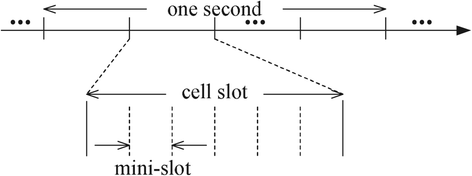
The TDMA transmission schedule.
-
(ii)
Mini-slot: since Lemma 3 suggests that there are at most \(\Theta (n\sqrt {a(n)})\) S-D lines passing through one cell, we further divide each cell slot into \(\Theta (n\sqrt {a(n)})\) mini-slots. So, each S-D pair hopping through it can use one mini-slot.

With the conflict-free transmissions by schedule our TDMA scheme, we can derive the achievable throughput and the delay. In particular, we have the following result.
Theorem 3.
For a random DIR network with n nodes, the achievable throughput is \(T(n)=\Theta \left (\frac {1}{k_{2} \sqrt {n \log n}}\right)\) and the average delay is \(D(n)=\Theta \left (\frac {1}{\left (\frac {4}{\tan ^{2}\frac {\theta }{2}}\right)^{\frac {2}{\alpha }}\sqrt {\frac {\log n}{n}}}\right)\).
Proof.
From the above the transmission scheduling scheme, each S-D pair can successfully transmit for \(\Theta \left (\frac {1}{k_{2} n\sqrt {a(n)}}\right)\) fraction of time. That is, the achievable throughput per S-D pair is \(T(n)=\Theta \left (\frac {1}{k_{2} n\sqrt {a(n)}}\right)\).
Then we calculate the average packet delay D(n). As defined before, the packet delay is the sum of the amount of time spent in each hop. First, we derive the bound on the average number of hops.
Since each hop covers a distance of r d (n), the number of hops per packet for S-D pair i is \(\Theta \left (\frac {d_{i}}{r_{d}(n)}\right)\), where d i is the length of S-D line i and r d (n) denotes the directional transmission range. Thus, the number of hops taken by a packet averages over all S-D pairs is \(\Theta \left (\frac {1}{n}\sum _{i=1}^{n}\frac {d_{i}}{r_{d}(n)}\right)\). Since for large n, the average distance between S-D pairs is \(\frac {1}{n}\sum _{i=1}^{n}d_{i}=\Theta (1)\), the average number of hops is \(\Theta \left (\frac {1}{r_{d}(n)}\right)\). As mentioned before, using directional antennas can extend the transmission range, i.e, \(r_{d}(n)=\left (\frac {4}{\tan ^{2}\frac {\theta }{2}}\right)^{\frac {2}{\alpha }} r(n)\), where r(n) is the transmission range by using omni-directional antennas. On the other hand, r(n) is bounded by the edge size of a cell, \(\sqrt {a(n)}\). Thus, the average number of hops is bounded by \(\Theta \left (\frac {1}{\left (\frac {4}{\tan ^{2}\frac {\theta }{2}}\right)^{\frac {2}{\alpha }}\sqrt {a(n)}}\right)\).
We then have the above result. □
From Theorem 3, since a(n) needs to be greater than \(2\frac {\log n}{n}\) to ensure the network connectivity, T(n) is still \(\Theta \left (\frac {1}{\sqrt {n \log n}}\right)\). But there is a capacity improvement factor \(\frac {1}{k_{2}}\), which is brought by directional antennas. Meanwhile, it is shown in Theorem 3 that \(D(n)=\frac {k_{2} n}{\left (\frac {4}{\tan ^{2}\frac {\theta }{2}}\right)^{\frac {2}{\alpha }}}T(n)\). We will show as follows that using directional antennas can also significantly reduce the delay compared with omni-directional antennas.
5.2 Discussions
We compare our results with those derived under OMN networks. First, we define the capacity gain factor to quantify the throughput capacity improvement induced by directional antennas.
Definition 4.
Throughput capacity gain factor. The capacity gain factor F T of a DIR network is the ratio of the maximum throughput of such network to that an OMN network, i.e., F T =T d (n)/T o (n), where T d (n) represents the achievable throughput of a DIR network consisting of n nodes, and T o (n) denotes the achievable throughput of an OMN network with the same number of nodes.
It is shown in [1,2,12], that the throughput of an OMN network is at most \(T_{o}(n)=\Theta \left (\frac {1}{\sqrt {n \log n}}\right)\). Thus, compared our derived result with that of an OMN network, the capacity gain can be calculated as follows.
Note that we ignore a factor depending on Δ during the above calculation since there is also a factor in T o (n) (refer to [1,2,12]).
When the path loss factor α=2, \(F_{T}=\frac {1}{8 \cdot \left (\frac {\theta }{2\pi }\right)^{2} \cdot \left (\frac {4}{\tan ^{2}\frac {\theta }{2}}\right)^{2}}\). When the antenna beam is quite narrow, i.e., beamwidth θ is quite small, \(\tan (\frac {\theta }{2})\approx \frac {\theta }{2}\). Thus, the capacity gain depends on θ 2, using directional antennas can significantly increase the network throughput. This result also conformed the previous finding in [3].
When α is larger, e.g., α=4, \(F_{T}=\frac {1}{\left (\frac {\theta }{2\pi }\right)^{2} \cdot \left (\frac {4}{\tan ^{2}\frac {\theta }{2}}\right)}\). When the antenna beam is quite narrow, \(\tan \left (\frac {\theta }{2}\right)\approx \frac {\theta }{2}\). In this case, there is a constant capacity improvement, which does not depend on the beamwidth θ. Thus, there is no significant capacity gain with directional antennas.
Our results imply that the improvement on the capacity by using directional antennas is also affected by the environmental factors such as the path loss factor α but not affected by the shadow fading effect.
We next analyze the delay reduction due to using directional antennas. Similarly, we define the delay reduction factor as follows.
Definition 5.
Delay reduction factor. The delay reduction factor F D of a DIR network is the ratio of the delay of such network to that one of an OMN network, i.e., F D =D d (n)/D o (n), where D d (n) represents the delay of a DIR network consisting of n nodes, and D o (n) denotes that of an OMN network with the same number of nodes.
It is shown in [2] that the delay an OMN network is at most \(D_{o}(n)=\frac {1}{\sqrt {a(n)}}\). Compared our result with that of an OMN network, the delay reduction factor can be calculated as follows.
As shown in Equation 17, when the path loss factor α=2, the delay reduction factor is \(\frac {1}{\frac {4}{\tan ^{2}\frac {\theta }{2}}}=\frac {1}{4}\tan ^{2}{\frac {\theta }{2}}\). When the beamwidth θ is small, the delay reduction factor is also quite small, which means that a narrow-beam antenna can significantly reduce the delay. When α is larger, e.g., α=4, the delay reduction factor is \(\frac {1}{\left (\frac {4}{\tan ^{2}\frac {\theta }{2}}\right)^{\frac {1}{2}}}=\frac {1}{2}\tan \left (\frac {\theta }{2}\right)\). When the antenna beam is quite narrow, the delay reduction factor also decreases although it does not decrease that much as the case with the lower path loss factor (e.g., α=2). The delay reduction of a DIR network mainly owes to the reduced number of hops in an ad hoc network.
6 Conclusions
In this paper, we investigate the throughput and the delay of wireless ad hoc networks using directional antennas (i.e., DIR networks). We have found that using directional antennas in wireless networks not only can improve the network throughput capacity but also can reduce the transmission delay induced by the multi-hop communications. The improvement on the network throughput of a DIR network mainly owes to the reduced interference by using directional antennas, which concentrate the signals in some directions. Besides, using directional antennas can significantly increase the transmission range, which results in the reduced number of hops and consequently leads to the reduction on the end-to-end delay.
Although directional antennas can significantly improve the network performance of wireless ad hoc networks, they also have a number of limitations which restrict the wide application of directional antennas in wireless ad hoc networks. For example, using directional antennas in wireless networks can lead to (1) the new carrier-sensing problems in MAC layer and (2) the node-localization problem [16]. So far as we know, there still lack of perfect solutions to the above issues. Besides, there are also a number of interesting problems implied by our results. For example, what is the scaling law with directional antennas when the mobility of nodes are considered? What is the impact of the side and back lobes of directional antennas on the transmission delay?
7 Endnotes
a In a random network, n nodes are randomly placed, and the destination of a flow is also randomly chosen. We only consider the random network in this paper.
b In an arbitrary network, the location of nodes, the antenna directions, and traffic pattern can be optimally controlled.
c In this paper, w.h.p. means that an event e happens with a high probability if P(e)→1 when n→∞.
8 Appendix 1
Proof of Lemma 1
Let A i be the event that cell i has at least one node and let m=1/a(n) be the number of cells. Then we have
Since \(m\leq \frac {n}{2\log n}\), we then have P(A i )≥1−1/n 2, which approaches 1 when n→∞. □
9 Appendix 2
Proof of Lemma 2
First, we consider an OMN network, in which a node in a cell transmitting omni-directionally to another node within the same cell or in one of its eight neighboring cells. Since each cell has area a(n), the distance between the transmitting and receiving nodes cannot be more than \(r_{o}=\sqrt {8a(n)}\) as shown in [2]. Thus, we require that R o ≤r o , where R o is the omni-directional transmission range. With the analysis of the effective transmission range in Section 1, we have the effective omni-directional transmission range, which is bounded by
We then extend this analysis to a DIR network and analyze the directional transmission range R d . As analyzed in Section 1, we can derive the effective directional transmission range E[ R d ] as follows
Compared with the effective omni-directional transmission range E[ R o ], the effective directional transmission range E[ R d ] is \(\left (\frac {4}{\tan ^{2}\frac {\theta }{2}}\right)^{\frac {2}{\alpha }}\) times longer. Specifically, we have
Under the interference model, a packet is successfully received if no node within distance I d of the receiver transmits at the same time, where I d is the directional interference range. It follows the interference model that the effective directional interference range E[ I d ] is
We next bound the number of interfering cells. In a DIR network, a node equipped with a directional antenna just concentrates its transmission to a certain direction, as shown in Figure 7. Thus, only cells covered by the antenna beam of the directional antenna can be interfered (the blue squares in Figure 7). Hence only the proportion of \(\frac {\theta }{2\pi }\) of cells can be interfered. Besides, since each receiver is also equipped with a directional antenna, it is interfered only when its antenna beam is pointed to the interferer. On average, the probability that a receiver is interfered is \(\frac {\theta }{2\pi }\). After applying the above analysis to the effective directional interference range, there are nearly \(\left (\frac {\theta }{2\pi }\right)^{2}\) times (E[ I d ])2/a(n) cells. More specifically, we have
Therefore, we have the above result. □
References
P Gupta, PR Kumar, The capacity of wireless networks. IEEE Trans. Inf. Theory. 46(2), 388–404 (2000).
A Gamal, J Mammen, B Prabhakar, D Shah, in Proc. of Twenty-third Annual Joint Conference of the IEEE Computer and Communications Societies (INFOCOM). Throughput-delay trade-off in wireless networks, (2004).
S Yi, Y Pei, S Kalyanaraman, in Proc. of the ACM International Symposium on Mobile Ad Hoc Networking and Computing (MobiHoc). On the capacity improvement of ad hoc wireless networks using directional antennas, (2003).
R Ramanathan, in Proc. of the ACM International Symposium on Mobile Ad Hoc Networking and Computing (MobiHoc). On the performance of ad hoc networks with beamforming antennas, (2001).
M Takai, J Martin, R Bagrodia, A Ren, in Proc. of the ACM International Symposium on Mobile Ad Hoc Networking and Computing (MobiHoc). Directional virtual carrier sensing for directional antennas in mobile ad hoc networks, (2002).
RR Choudhury, X Yang, NH Vaidya, R Ramanathan, in Proc. of the Annual International Conference on Mobile Computing and Networking (MOBICOM). Using directional antennas for medium access control in ad hoc networks, (2002).
L Bao, J Garcia-Luna-Aceves, in Proc. of the Annual International Conference on Mobile Computing and Networking (MOBICOM). Transmission scheduling in ad hoc networks with directional antennas, (2002).
T Korakis, G Jakllari, L Tassiulas, in Proc. of the ACM International Symposium on Mobile Ad Hoc Networking and Computing (MobiHoc). A MAC protocol for full exploitation of directional antennas in ad-hoc wireless networks, (2003).
Z Zhang, in Proc. of IEEE International Conference on Communications (IEEE ICC). Pure directional transmission and reception algorithms in wireless ad hoc networks with directional antennas, (2005).
R Ramanathan, J Redi, C Santivanez, D Wiggins, S Polit, Ad Hoc Networking With Directional Antennas: A Complete System Solution. IEEE J. Select. Areas Commun. 23(3), 496–506 (2005).
HN Dai, KW Ng, RCW Wong, MY Wu, in Proc. of the 27th IEEE Conference on Computer Communications (INFOCOM). On the Capacity of Multi-Channel Wireless Networks Using Directional Antennas, (2008).
AE Gamal, J Mammen, B Prabhakar, D Shah, Optimal throughput-delay scaling in wireless networks-part I: The fluid model. IEEE Trans. Inf. Theory. 52(6), 2568–2592 (2006).
S Toumpis, AJ Goldsmith, in Proc. of Twenty-third Annual Joint Conference of the IEEE Computer and Communications Societies (INFOCOM). Large Wireless Networks under Fading, Mobility and Delay Constraints, (2004).
MJ Neely, E Modiano, Capacity and Delay Tradeoffs for Ad-Hoc Mobile Networks. IEEE Transactions on Information Theory. 51(6), 1917–1935 (2005).
HN Dai, in Proc. of Fifth International Conference on Intelligent Sensors, Sensor Networks and Information Processing (ISSNIP). Throughput and delay in wireless sensor networks using directional antennas, (2009).
HN Dai, KW Ng, M Li, MY Wu, An Overview of Using Directional Antennas in Wireless Networks. Int. J. Commun. Syst. (Wiley). 26(4), 413–448 (2013).
TS Rappaport, Wireless communications: principles and practice, second edition (Prentice Hall PTR, Upper Saddle River, NJ, USA, 2002).
A Goldsmith, Wireless Communications, first edition (Cambridge University Press, Cambridge, United Kingdom, 2005).
W DD Wackerly, RL Mendenhall, Scheaffer, Mathematical Statistics With Applications, seventh edition (Cengage Learning, Independence, KY, USA, 2007).
C Bettstetter, C Hartmann, Connectivity of Wireless Multihop Networks in a Shadow Fading Environment. ACM Wireless Networks. 11(5), 571–589 (2005).
Acknowledgements
The work described in this paper was supported by Macao Science and Technology Development Fund under Grant No. 036/2011/A, Grant No. 081/2012/A3 and Grant No. 096/2013/A3. The authors would like to thank Gordon G.-D. Han for his excellent comments.
Author information
Authors and Affiliations
Corresponding author
Additional information
Competing interests
The authors declare that they have no competing interests.
Rights and permissions
Open Access This article is distributed under the terms of the Creative Commons Attribution 4.0 International License (https://creativecommons.org/licenses/by/4.0), which permits use, duplication, adaptation, distribution, and reproduction in any medium or format, as long as you give appropriate credit to the original author(s) and the source, provide a link to the Creative Commons license, and indicate if changes were made.
About this article

Cite this article
Dai, HN., Zhao, Q. On the delay reduction of wireless ad hoc networks with directional antennas. J Wireless Com Network 2015, 16 (2015). https://doi.org/10.1186/s13638-015-0248-y
Received:
Accepted:
Published:
DOI: https://doi.org/10.1186/s13638-015-0248-y