PCAC: Power- and Connectivity-Aware Clustering for Wireless Sensor Networks

Abstract

In this article, we investigate clustering algorithms that are proposed for wireless sensor networks (WSNs). Then, we propose a clustering algorithm for WSNs called PCAC, that is both power and connectivity aware. Our proposed Power- and Connectivity-Aware Clustering (PCAC) algorithm provides higher energy efficiency and increases the total life time (TLT) of the network. We evaluate our proposed PCAC algorithm in a simulation environment and compare its performance to previously proposed algorithms. According to the simulation results, our proposed PCAC algorithm is energy efficient and also provides longer TLT (in worst-case, up to 85% improvement for a 15-node network with one-hop connectivity) to the network, compared to the previously proposed algorithms.

1 Introduction

Wireless sensor networks (WSNs) continue to grow as one of the most exciting and challenging research areas of engineering. There are many applications of WSNs, which are intended to monitor physical and environmental phenomena, such as earthquake, pollution, wild fire, water quality and to gather information regarding human activities in health care, manufacturing machinery performance, building safety, military surveillance and reconnaissance, highway traffic, etc. [1].

WSNs are characterized by severely constrained computational and energy resources, and an ad hoc network operational environment. They pose unique challenges, due to limited power supplies, low transmission bandwidth, small memory sizes, and limited energy; therefore, networking techniques used in traditional networks cannot be adopted directly [2]. So, new ideas and approaches (algorithms) are needed in order to increase the overall performance of the network, especially in terms of total life time (TLT). Clustering, is one of those techniques that is very useful for WSNs in data aggregation and filtering and is the main focus of this paper.

A clustered WSN is typically as shown in Figure 1. Each cluster is a group of interconnected sensor nodes with a dedicated node called cluster head (CH). CHs are responsible for the management of the cluster such as scheduling of the medium access, dissemination of the control messages, and, the most important, data aggregation. The size of a cluster is defined as the hop distance from the CH to the farthest node in the cluster. For example, in a three-hops cluster, the distance between the CH and the farthest node is three-hops (four nodes are in the path including the end points). The clustered network shown in Figure 1 has a one-hop distance in between CHs and the member sensor nodes.

Figure 1

A typical clustered WSN.

Clustering is the process of grouping the nodes in a network that are within a specified hop distance or have some shared common properties into clusters and electing CHs for each cluster. This election can be made permanent (static clustering) or repeated in some certain time intervals (dynamic clustering). Clustering is used in many applications of wireless sensor networks in order to reduce the traffic load on the nodes through data aggregation process, to prolong total network life time, to balance the data traffic in the network, and finally to increase the scalability (allows the deployment of hundreds or thousands of nodes). Besides, clustering helps us to increase security of the network by allowing implementation of complex cryptography algorithms. By using a clustered networking approach, power-consuming algorithms (such as data aggregation and encryption) would be run on the CHs, and this would help us to improve the TLT of the network significantly.

In this article, we investigate clustering algorithms that are proposed for WSNs and propose a new clustering algorithm that is both power and connectivity aware. The rest of the paper is organized as follows: Section 2 provides a description of the related work available in the literature. Section 3 presents Kachirski et al.’s connectivity-aware clustering algorithm, and Section 4 provides the revised and improved version of that algorithm. Our proposed Power- and Connectivity-Aware Clustering (PCAC) algorithm is presented in Section 5. Section 6 provides the comparison of both schemes and also presents the details of our simulation environment. In Section 7, we discuss the observations regarding the effects of the clustering on the performance of the WSNs. Finally, Section 8 concludes the paper and outlines future work.

2 Related work

There are plenty of clustering algorithms available in the literature that are proposed for wireless networks. In this section, we present the most widely used clustering algorithms and mention their advantages and disadvantages:

Low-Energy Adaptive Clustering Hierarchy (LEACH) [3] is a distributed clustering algorithm in which nodes make autonomous decisions without any centralized control. Cluster formation is cyclically performed and history information of the previous CHs are stored. CHs are assigned as a result of a random procedure, where each node can declare itself as a CH with some probability. Energy levels of the nodes are included as a factor in the CH selection while connectivity of the nodes are ignored. Therefore, it is not guaranteed that every node is within K-hops of a CH. This is the main concern of LEACH, which may cause some nodes to be segregated from the rest of the network during the time period in between the two election cycles. Another drawback of LEACH is due to the assumptions that not only the network size and the number of CHs are known in advance but also all nodes are very well synchronized (in order to ensure that CHs can be re-elected periodically to balance the energy consumption). These are very specific assumptions that might not fit well to real-life applications, especially for WSNs.

In [4], Bandyopadhyay et al. propose a distributed and randomized clustering algorithm similar to the LEACH. The proposed algorithm also aimed at energy efficiency, and its difference from the LEACH is that it provides hierarchical (multi-level) clustering as well. Other than that, the proposed algorithm holds the same concerns and drawbacks as LEACH does.

In [5], Jia et al. present an energy-consumption-balanced clustering algorithm (LEACH-EP) for WSNs that is based upon the LEACH algorithm. It introduces an energy factor in the CH-electing threshold and optimizes the election probability of CH. As in the case of LEACH, LEACH-EP comes with specific assumptions as well. As in the case of LEACH, these specific assumptions might not fit well to real-life applications of WSNs.

Energy-Efficient Clustering Scheme (EECS) [6] is also based upon the LEACH algorithm and aims at energy efficiency. Its difference from the LEACH is the setup phase of the clusters (cluster formation). LEACH-C [7] and SECA [8] are also based on the LEACH algorithm. Both algorithms consider node-positions into account while calculating the CHs and try to cumulate the clusters. All of these LEACH-based proposed algorithms hold the same concerns and drawbacks as LEACH does.

In Hybrid, Energy-Efficient, Distributed Clustering (HEED) [9] approach, CHs are periodically selected according to a hybrid of their residual energy and a secondary parameter, such as a node’s proximity to its neighbors or node degree. HEED does not make any assumptions about the distribution or the density of the nodes, nor their connectivities.

Evenly Distributed Clustering (EDC) algorithm [10] distributes clusters uniformly and minimizes the number of clusters. It considers the connectivity of the nodes with the K-hops parameter. It is a heuristic approach, in which each node only exchanges its head selection with its neighbors. Based on neighbors’ selection results, each node chooses the nearest head as its CH. The drawback of this algorithm is that it does not consider the density of the nodes in a network. In order to increase the TLT of the network, it is important to elect more CHs in the dense areas of the network. However, the algorithm is aimed at distributing the cluster heads evenly to the network deployment field.

In [11], Brust et al. present algorithms for cluster head candidate selection that are based on topology (location) of the nodes. The algorithms aim to avoid selecting nodes located close to the network partition border because those nodes are more likely to move out of the partition, thus, causing a CH re-election. By using the connectivity information, they propose three algorithms to find the strong, weak, bridge, and board nodes in the network. Authors do not provide any information on how to select the CHs among their selection of nodes (strong, weak, bridge, and board nodes). Overall, this classification of nodes for CH selection would be useful for the mobile ad hoc networks (MANETs) where mobility is the prime factor that changes the network topology. However, the network topology in WSNs is quite stable compared to MANETs, and therefore, this kind of node classification is unnecessary and also expensive (power consuming) for CH selection.

Energy-Efficient Unequal Clustering (EEUC) [12] is proposed for periodically data-gathering WSNs. It partitions the nodes into clusters of unequal size, and clusters closer to the base station have smaller sizes than those farther away from the base station. This way, CHs closer to the base station can preserve some energy for inter-cluster data forwarding.

Hierarchical clustering proposed in [13] is a framework based on two-level clustering, multi-hops clusters for data aggregation (the first-level clustering), and one-hop clusters for intrusion detection (the second-level clustering). Although the idea sounds promising for some applications of WSNs (especially for the industrial applications), the details of the formation algorithms for the multi-level clustering were missing (we assume that this was left as a future work).

Kachirski et al.’s [14] clustering algorithm is based on the connectivity of the nodes in the network. The higher the connectivity (neighbors) a node has, the higher the probability of it to be elected as the CH of a certain neighborhood (cluster). This algorithm is one of the best choices for us to work on for several reasons: first of all, it did not require probabilistic approach on clustering, and therefore, the result of the clustering would cover the whole network. Secondly, the connectivity of the nodes are the main concern on the election of CHs, which is reasonable. In general, the nodes that have more connections would be rather elected as CHs. Finally, the algorithm is easily implementable, which allows the proof of the theoretical work on both hardware and simulation environment.

There are flaws in Kachirski et al.’s [14] clustering algorithm: 1) nodes were not able to vote for themselves through the election phase of the CHs. Thus, we fixed this problem and called it as ‘revised version of Kachirski et al.’s algorithm’. We showed geographically how this change would result in a more logical cluster formation. 2) There was no power awareness in their proposed algorithm. Therefore, in this article, we propose our clustering algorithm that is built upon the revised version of Kachirski et al.’s algorithm. Our proposed PCAC algorithm is both power and connectivity aware, that is why it provides maximum throughput while saving the energies of the nodes, therefore, significantly increasing the TLT of the network.

3 Kachirski et al.’s connectivity-based approach for clustering

In order to demonstrate the principles of the Kachirski et al.’s [14] clustering algorithm, consider the network shown in Figure 2. Here, we assume that each node has one-hop^a connectivity, meaning that each node can communicate with its direct neighbors that are in one-hop communication distance (in terms of radio range). In order to elect the CHs, these are the steps to be followed:

Figure 2

A typical 9-node WSN.

• 1. Let C _i denote the number of established connections (nodes that are one-hop away in our case) for node i, with total number of N nodes in the network. Each node calculates its own C _i value (as shown in Figure 3; note that the number written in each node represents the total number of neighbors for each node) and sends it to all its neighbors.

  Figure 3

  

  Established connections graph, indicating total number of one-hop neighbors for the WSN shown in Figure 2.

• 2. After receiving C _k values from its neighbors k (where k≠i for all i=1…N), a node i calculates the connectivity index (S _i ) as shown in Equation 1:

  $$ S_{i} = C_{i} + \sum\limits_{k}{C_{k}} $$

  ((1))

  Each node calculates its own connectivity index according to Equation 1. For the network shown in Figure 3, the connectivity indices would be as shown in Figure 4.

  Figure 4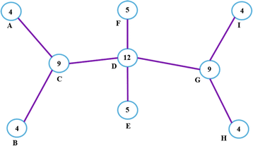

  

  Connectivity index graph (one-hop) of the WSN shown in Figure 2.

• 3. Each node broadcasts its connectivity index (S _i ) to all other nodes with a time to live (TTL) value equivalent to time spent through one-hop communication.

• 4. Each node then has to participate in a voting session in which the CH will be determined. Each node votes for the node that has the highest S _i value, as a result of the broadcast operation in step 3.

• 5. After the voting procedure, if a node receives at least one vote, it is assigned as the CH. After the voting session, the network members in Figure 4 select their CHs as shown in the Figure 5 ^b.

  Figure 5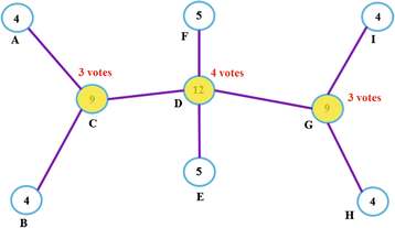

  

  Elected CHs (one-hop) and their votes, after the voting session for the WSN shown in Figure 2.

4 Revised version of Kachirski et al.’s connectivity-based approach for clustering

In the specific case of the network shown in Figure 2, there are nine members of the network, and three members (out of nine) are elected as cluster heads, as a result of the voting procedure (see Figure 5). As the network connectivity increases, we expect to have more connected members in the network resulting in less number of selected CHs. As an example, for the same configuration of the network in Figure 2, if we use two-hops connectivity for the node communications, we obtain the neighborhood graph as shown in Figure 6. By applying Equation 1 and then performing the voting session, the connectivity index graph (denoted on the nodes) and the CH selections would be as shown in Figure 7 ^b.

Figure 6

Established connections graph, indicating total number of two-hops neighbors for the WSN shown in Figure 2.

Figure 7

Connectivity index graph and elected CHs (two-hops) of the WSN shown in Figure 2.

This is quite an interesting result, since we were expecting to have less CHs by increasing the connectivity (number of maximum hops). This happens because of a fault in the voting procedure of Kachirski et al.’s [14] clustering algorithm. We realized that throughout the voting procedure, nodes are not voting for themselves even though they may have the highest connectivity. This may result in more CHs to be elected than needed. In order to fix this problem, we revised Kachirski et al.’s clustering algorithm by letting the nodes vote for themselves (if they have the highest connectivity index).

We applied the revised scheme to our example network (see Figure 2), and the result of the voting scheme is as shown in Figure 8 ^b. Here, the total number of CHs is one, resulting in less CHs (instead of three) compared to the original Kachirski et al.’s clustering algorithm, as expected (the fault is fixed).

Figure 8

Elected CHs (two-hops) of the WSN shown in Figure 2 by using the revised clustering scheme.

5 PCAC: Power- and Connectivity-Aware Clustering

In WSNs, energy is one of the scarce resources that needs to be conserved. As a result of the clustering algorithms, elected cluster heads become the highest energy-consuming nodes of the network, since they perform operations related to data aggregation, security, routing, etc., on behalf of other nodes.

Kachirski et al.’s [14] clustering algorithm (see Section 3), and it’s revised version (see Section 4) only consider a node’s connectivity with its neighbors while determining a CH. But they do not consider any parameter regarding the energies (nor the powers) of the nodes.

In order to increase the TLT of a WSN, energy (power) levels of the nodes also should be considered while determining the CHs. Therefore, in this section of our paper, we propose the PCAC algorithm built upon the revised version of (see Section 4) Kachirski et al.’s [14] clustering algorithm. We achieved this by introducing the power-level readings through connectivity index calculations (see Section 3, step 2). Our scheme determines the CHs according to these calculations. Besides, the voting scheme follows the revised version of Kachirski et al.’s clustering algorithm (nodes may vote for themselves).

The description of our proposed scheme is as follows:

• 1. Let C _i denote the number of established connections for node i, with total number of N nodes in the network. Each node calculates its own C _i value and sends it to all its neighbors.

• 2. After receiving C _k values from its neighbors k (where k≠i, for all i=1…N), a node i calculates the connectivity index (S _i ) as shown in Equation 2:

  $$ S_{i} = C_{i} + \sum_{k}{C_{k}} + \beta \times P_{i} $$

  ((2))

  In this equation, β is called power factor, and the P _i value represents the battery power level of each node i. β represents the correlation of the power level of each node (P _i ) to the connectivity index (S _i ) of that particular node. By this way, whenever a centrally located node starts to deplete its battery power, it is guaranteed that it will not be elected as a CH in the next CH-election phase. Equation 2 describes how, in our PCAC algorithm, each node’s connectivity index (S _i ) not only carries information regarding its connectivity (C) with its neighbors, but also the battery power level (P _i ) of that particular node.

  In our calculations, maximum value for P _i is chosen as 1.00, meaning that the battery power level of the node is 100% of its maximum level. For the given WSN shown in Figure 2, the connectivity indices and the voting results are shown in Figure 8. We recalculate the connectivity indices for that network according to Equation 2, and the new results are shown in Figure 9. Here, each green writing over the nodes represents the battery power level (percentage) of that node at the time that the clustering calculation is done.

  Figure 9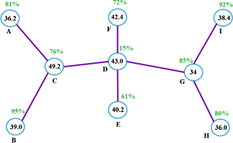

  

  Connectivity index graph (two-hops) of WSN shown in Figure 2, as a result of our PCAC algorithm.

• 3. Each node broadcasts its connectivity index (S _i ) to all other nodes with a TTL value equivalent to time spent through one-hop communication. TTL helps the network to prevent packet-replay attacks. Besides, TTL is used to discard late-arriving votes (because of network congestion) and lets the voting procedure be completed in a timely manner.

• 4. Each node then has to participate in a voting session in which the CH will be determined. Each node votes for the node that has the highest S _i value (nodes are allowed to vote for themselves), as a result of the broadcast operation in step 3.

• 5. After the voting procedure, if a node receives at least one vote, it is assigned as the CH. After the voting session, the network members in Figure 9 select their CHs as shown in the Figure 10 ^b.

  Figure 10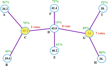

  

  Elected CHs (two-hops) of the WSN shown in Figure 2 by using our PCAC algorithm.

5.1 Observations on TLT, β, and τ

TLT is the most important parameter in WSNs. It determines the life time of the network. In our calculations and throughout this paper, TLT is determined as follows: whenever a node’s battery power depletes and disconnects from the network, its life time is considered as TLT of the network. In order to distinguish dead nodes from disconnected nodes, we use battery-low signal; whenever a node’s battery goes into weak stage, it broadcasts a ‘low battery’ message to all neighbors. If a neighbor disconnects after this message, then we consider this as the end of the network operation. Otherwise, the network resumes operation.

Energy consumption and TLT are inversely proportional: the more energy consumption a node has, the less TLT it will have. Both parameters are correlated to connectivity as follows: the higher the connectivity index (S _i ) of a node, the more messages (or packets) will pass through it. This means more transmissions consuming more node energy, thereby depleting its battery power (P _i ) faster. Therefore, TLT of the network is also reduced.

When a WSN uses our proposed PCAC algorithm, we expect two parameters to effect the TLT of thenetwork:

• Power factor (β): an optimum value of β can be determined by keeping every parameter in the network fixed and then by observing the TLT of the network with the change of β.

• Period of clustering (τ): it is the time period that determines the renewal of the cluster heads by re-applying the clustering algorithm. An optimum value of τ can be determined by keeping every parameter in the network fixed and then by observing the TLT of the network with the change of τ.

As an example, we simulated our PCAC algorithm on the network shown in Figure 9 with the simulator discussed in the next section (Section 6). Figure 11 shows the behavior of the TLT with the change of β, whereas Figure 12 shows the behavior of the TLT with the change of τ. According to the result of the simulations, we may conclude that, for the network configuration of Figure 9 and the parameter selection shown in Section 6.2, the optimum value of β is 200 (the TLT curve in Figure 11 saturates for β≥200) and the optimum value of τ is 45 (the TLT curve in Figure 12 gets the maximum value at τ=45 and starts decreasing as τ becomes bigger or smaller than this value).

Figure 11

Total life time vs. beta, for the WSN shown in Figure 2 by using our PCAC algorithm.

Figure 12

Total life time vs. period of clustering, for WSN shown in Figure 2 by using our PCAC algorithm.

5.2 Applicability of our proposed PCAC algorithm to nowadays WSNs

Our proposed PCAC algorithm is very applicable to nowadays WSNs. Because, current Commercial Off-The-Shelf (COTS) nodes, such as Wasp motes [15], provide the power reading of it’s batteries (as a percentage) as an available information which could be sent to other nodes. This information would be used directly by our proposed PCAC algorithm in order to determine the cluster heads.

6 Comparison of both schemes in terms of total life time of the WSN

In order to evaluate and compare the effect of both Kachirski et al.’s (revised) clustering algorithm and our proposed PCAC algorithm on the total life time of the WSNs, we created a simulation environment in M A T L A B ^TM[16]. The details of the simulation environment and the theoretical background are as follows:

6.1 Energy-consumption calculations

For energy-consumption calculations, we followed Heizelman et al.’s work [7]. We assume a simplified model (since radio wave propagation is mostly non-stable and difficult to model) for the radio hardware energy dissipation, where the transmitter dissipates energy by running the radio electronics and the power amplifier, whereas the receiver dissipates energy by running the radio electronics only, as shown in Figure 13.

Figure 13

Radio-energy-dissipation model used in our simulations [7].

We consider two different channel models depending on the distance between the transmitter and the receiver:

• 1. Near-field (free space - fs) channel model: if the distance between the transmitter and the receiver is less than a threshold (d ₀), then this model is used (also called d ² power-loss model).

• 2. Far-field (multi-path - mp) channel model: if the distance between the transmitter and the receiver is greater than a threshold (d ₀), then this model is used (also called d ⁴ power-loss model).

According to [5], the threshold value for the distance is calculated as follows:

$$ d_{0} = \frac{\sqrt{\epsilon_{\text{fs}}}}{\sqrt{\epsilon_{\text{mp}}}} $$

((3))

where ε _fs and ε _mp are constants related to free-space loss and multi-path loss, respectively.

In order to transmit m-bit data to a distance of d, the radio spends:

$$\begin{array}{*{20}l} E_{Tx}(m,d) &= E_{Tx-\text{elec}}(m) + E_{Tx-\text{amp}}(m,d)\\ &= \left\{ \begin{array}{ll} mE_{\text{elec}} + m\epsilon_{\text{fs}}d^{2}, & d < d_{0}\\ mE_{\text{elec}} + m\epsilon_{\text{mp}}d^{4}, & d \geq d_{0} \end{array} \right. \end{array} $$

((4))

In order to receive the same m-bit data, the radio spends:

$$ E_{Rx}(m) = E_{Rx-\text{elec}}(m) = mE_{\text{elec}} $$

((5))

The energy spent on the radio electronics circuitry, E _elec, is due to the digital modulation (transmitter side), digital demodulation (receiver side), error correction codes, and filtering, whereas the amplifier energy, E _{T x−amp}, is due to the electromagnetic spreading of the signal into the air and depends on the distance as mentioned above (see Equation 3).

Assume that each CH has N member nodes. CH dissipates energy by receiving the data from member nodes, aggregating those data, and finally transmitting the aggregate data to the base station (BS). We assume that BS is located far away from the nodes, and therefore, transmission between the CH and the BS follows the far-field channel model (d ⁴ power-loss model). During a single data frame, we calculate the energy dissipated in the CH as follows:

$$ \begin{aligned} E_{CH} & = \{E_{\text{aggregating\_data\_from\_member\_nodes}}\} \\ &\quad+ \{E_{\text{transmit\_aggregate\_data\_to\_BS}}\} \\ & = \{N (mE_{\text{elec}} + mE_{\text{DA}})\} + \left\{mE_{\text{elec}} + m \epsilon_{\text{mp}} d_{\text{toBS}}^{4}\right\} \end{aligned} $$

((6))

where m represents the total number bits in a data frame, m E _DA represents the energy dissipated during aggregating m-bit data, and finally d _toBS represents the distance between the CH and the BS.

Assume that each member node is located in the near field of the CH so that near-field channel model (d ² power-loss model) will be used for calculating the energy dissipated during data transmission from the member node towards the CH. Therefore, we calculate the energy dissipated in each member node as follows:

$$ E_{\text{member\_node}} = mE_{\text{elec}} + m \epsilon_{\text{fs}} d_{\text{toCH}}^{2} $$

((7))

where d _toCH represents the distance between the member node and the CH, and therefore, it takes different values for each node.

For all our simulations referred in our work, we followed the energy-consumption models of [7] and used the values for the energy-consumption-related parameters as shown in Table 1.

Table 1 Values for the energy-consumption-related parameters used through our simulations

6.2 Simulation parameters

The parameters that we used during the simulation are as follows:

• Each node in the network is identical to each other and has a starting energy of 2 J.

• There is a BS located outside of the network to collect the data from CHs.

• The deployment area is 100 m×100 m.

• Data flow from nodes to CHs. CHs aggregate the data and then forward to the BS.

• The header size for each frame is 200 bits.

• The data size for each frame is 4,000 bits.

• Data rate is 1 frame per 10 min (0.1 frames/min).

• We consider a packet drop rate of 5% for the transmission of each data frame due to the collisions and multi-path fading.

• We consider a stationary network meaning that both BS and the nodes are not moving.

• Each simulation is run 1,000 times, and an average value of the total life time (that falls into 95% confidence interval) is calculated. For example, for the simulation result presented in Section 6.4 (energy consumption graph of Kachirski et al.’s clustering algorithm), the distribution of the total life time is shown in Figure 14. Here, the lower bound and upper bounds of the confidence interval (95%), as well as the mean value, are shown on the graph. Figures 15 and 16 show the corresponding histogram plot and quantile-quantile plot, respectively. In these figures, the first plot represents our simulation data, and the second plots represent the normal distribution (Gaussian) that has the same mean value as our data. From these figures, we observe that our simulation result shows a normal distribution (in the quantile-quantile plot, our data cumulates on the x = y line). Therefore, we calculated the mean value for each simulation in this text to represent all the values resulted in 1,000 iterations.

  Figure 14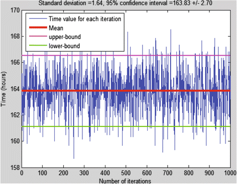

  

  Distribution of the simulation time.

  Figure 15

  

  Histogram plots of the simulation time compared to the normal distribution.

  Figure 16

  

  Quantile-quantile plots of the simulation time compared to the normal distribution.

6.3 Location of the nodes

Throughout our simulations, we assumed that both BS and the nodes are stationary; therefore, their positions are fixed. For the following sections, positions of the nodes and the BS will be as shown in Figure 17. Here, circular shapes represent the nodes (blue ones are the member nodes and the red ones are the CHs) CHs) whereas the square shape represents the BS. The red lines represent the connection between the CHs and the BS, whereas the blue lines represent the connections between the CHs and their member nodes. The whole deployment area is 100 m×100 m, and the location of the BS is [100 m, 100 m]. The nodes are deployed to the area with the following boundaries: [10 m, 10 m],[10 m, 30 m],[50 m, 10 m], and [50 m, 30 m].

Figure 17

Location of the nodes and the BS throughout the simulations.

6.4 Energy consumption of Kachirski et al.’s clustering algorithm (revised version)

We ran the revised version of Kachirski et al.’s clustering algorithm on our simulator with the parameters shown in Section 6.2 and the positions shown in Section 6.3. We considered one-hop connectivity for all nodes in the network. Figure 18 shows the total number of neighbors for each node (including the connection paths), connectivity indices, and results of the voting along with the elected CHs.

Figure 18

CH selection of a nine-node WSN with Kachirski et al.’s algorithm (revised version).

Figure 19 shows the energy-consumption performance of the mentioned algorithm with respect to time. We stopped the simulation whenever a single node dies (runs out of battery power), and we call this time as the ‘total life time of the network’, since at this point the network starts to disintegrate (segregation starts).

Figure 19

Energy consumption graph of Kachirski et al.’s clustering algorithm (revised version).

In Figure 19, we can see that node 8 depleted its energy faster than other nodes and therefore determined the network’s total life time as 163.8 h.

6.5 Energy consumption of our proposed PCAC algorithm

We ran our proposed PCAC algorithm on our simulator with the parameters shown in Section 6.2 and the positions shown in Section 6.3. We consider one-hop connectivity for all nodes in the network. As mentioned in Section 5, we selected β as 200 and τ is 45, in order to achieve the maximum TLT. Figure 20 shows the result of the clustering algorithm at times t=0 and t=t ₁(t ₁>0). Figure 21 shows the energy-consumption performance of our proposed algorithm with respect to time. In Figure 21, we can see that node 7 depleted its energy faster than other nodes and therefore determined the network’s TLT as 316.66 h. When compared to the revised version of Kachirski et al.’s clustering algorithm (see previous sub-section), relative performance improvement in TLT of the network is 93%.

Figure 20

CH selection of a nine-node WSN with our algorithm; (left) at time t=0, (right) at time t=t ₁(t ₁>0).

Figure 21

Energy-consumption graph of our PCAC algorithm.

6.6 Further comparisons

In order to provide further proof of performance improvement on life time, we repeated the same simulation setup with different network topologies with 7 nodes, 9 nodes, and finally 15 nodes (see Figure 22). We ran both clustering algorithms on these networks in three different maximum number of hops: one, two, and three. The resulting relative performance improvements on the total life time of the network are as shown in Table 2. Accordingly, we conclude that, as the maximum number of hops increases, our clustering algorithm becomes more beneficial. This is because more nodes become eligible to be elected as CHs as the maximum number of hops increases. According to our simulations, the relative performance improvement of clustering algorithm varies between 85% and 93% for one-hop neighborhood, 234% and 313% for two-hops neighborhood, and finally 366% and 463% for three-hops neighborhood, respectively.

Figure 22

Different network topologies with 7 and 15 nodes.

Table 2 Relative performance improvements (%) on the life time of the network when our PCAC algorithm is used

7 Some observations on the effect of clustering to the network performance

7.1 Effect of maximum number of hops on total number of cluster heads

As the maximum number of hops increases, the nodes in the network achieve more communications with the other member nodes, and as a result, the network requires less number of CHs. To support this hypothesis, we ran the CH selection algorithm on a 15-node network for three different maximum number of hops: one, two, and three. The resulting total number of neighbors, connectivity indices, voting results, and the elected CHs are shown in Figures 23, 24, and 25, respectively.

Figure 23

Clustering of 15-node network, one-hop communication case.

Figure 24

Clustering of 15-node network, two-hops communication case.

Figure 25

Clustering of 15-node network, three-hops communication case.

Accordingly, Figure 26 shows the plot of maximum number of hops versus the total number of elected CHs, for a 15-node network.

Figure 26

Maximum number of hops vs. total number of CHs for a 15-node network.

7.2 Effect of total number of cluster heads (maximum hops) on the total life time of the network

The positions of the BS and the WSN nodes are as shown in Figure 27. BS is located in the far field of the WSN, meaning that the distance between CHs and the BS is greater than 87.7 m. The simulation parameters are the same as shown in Section 6.2. β is chosen as 200 and the τ as 40 frames. By using these parameters and positions, we ran the simulation for four cases of the maximum hops: zero, one, two, and three. Figure 28 shows the behavior of TLT of the network with respect to maximum hops. Accordingly, we conclude that, as the maximum hops increases, the TLT of the network increases. From the slope of the curve, we can deduce that this increase saturated at a certain number of hops. This is the point where each node can reach any node in the network (six-hops in this case).

Figure 27

Location of the nodes and the BS.

Figure 28

Maximum hops vs. total life time of the network.

7.3 Effect of total number of nodes in a cluster on total life time of the network

We wondered about the effect of total number of the nodes in the network on the TLT of the network. To investigate this, we considered the same network shown in Figure 27 along with the simulation parameters the same as Section 7.2. The only parameter that is different here is the maximum hops. We kept it constant and equal to three. Then, we started the simulation with 15 nodes, and then, each time, we removed one of the end nodes and repeated the simulation till we are left with one node in the network. As a result, Figure 29 shows the behavior of the TLT of the network with respect to the total number of nodes in the network. Accordingly, we conclude that there is a certain number of nodes (six nodes in our case) in the network that allow the network to achieve maximum TLT (519.15 h in our case).

Figure 29

Total number of nodes vs. total life time of the network.

7.4 Effect of data rate on the total life time of the network

Here, we investigated the effect of frame rate of the nodes in the network on the TLT of the network. We considered the same network shown in Figure 27 along with the simulation parameters the same as Section 7.2. The only parameter that is different here is the maximum hops. We kept it constant and equal to three. Then, we started the simulation with 15 nodes, and then, each time, we changed the frame rate and repeated the simulation for various frame rates. As a result, Figure 30 shows the behavior of the TLT of the network with respect to the frame rate of the nodes in the network. Accordingly, we conclude that, as the frame rate increases, TLT decreases. This is an expected result, because, as the frame rate increases, more packets are sent between the nodes thus more energy is consumed.

Figure 30

Frame rate vs. total life time of the network.

7.5 Conclusions from the observations

There are three major trade-off situations that need to be balanced when implementing solutions (i.e., security, etc.) to a clustered WSN:

• 1. There is a trade-off between ‘maximum hop count’ and ‘total number of CHs’. As the maximum hop count increases, total number of CHs decreases and vice versa.

• 2. There is a trade-off between ‘total number of CHs’ and ‘TLT of the network’. There is an optimum number of CHs which lead the network to survive the most TLT possible (without having any partioning/segregation).

• 3. There is a trade-off between ‘data rate (frames/minute)’ and ‘TLT of the network’. As the data rate increases, more data need to be processed and more packets need to be transmitted causing more power to be spent; therefore, the TLT of the network decreases.

8 Conclusions

In this work, we provided the energy-consumption simulation results of the revised version of Kachirski et al.’s clustering algorithm and our proposed PCAC algorithm. According to these results, our proposed PCAC algorithm out-performed the revised version of Kachirski et al.’s clustering algorithm in terms of energy efficiency and also total life time of the network.

According to our simulation results, with our proposed PCAC algorithm, relative performance improvement (compared to the revised version of Kachirski et al.’s clustering algorithm) in total life time of the network varies between 85% and 93% for one-hop neighborhood, 234% and 313% for two-hops neighborhood, and finally 366% and 463% for three-hops neighborhood, respectively.

Here, we note that mobility can also be included as an another parameter in CH calculations (in Equation 2) for MANETs. For example, highly mobile nodes (Wasp motes [17] provide three-axis accelerometer reading which would be used to measure mobility) may be elected as CHs, because they might be in contact with most of the nodes in a certain amount of time. Since WSNs are mostly stationary, we did not consider any mobility in our calculations and left this part as a future work to be considered.

9 Endnotes

^a The same method would be applied in the case of multiple-hops (2,3,…, etc.) connections if needed.

^b CHs are highlighted with yellow color and also the votes they received are noted on top of them in red color writing.

References

I Butun, Y Wang, Y Lee, R Sankar, Intrusion prevention with two-level user authentication in heterogeneous wireless sensor networks. Int. J. Secur. Netw. 7(2), 107–121 (2012).
I Butun, S Morgera, R Sankar, A survey of intrusion detection systems in wireless sensor networks. Commun. Surv. Tutorials. 16(1), 266–282 (2013).
WR Heinzelman, A Chandrakasan, H Balakrishnan, in System Sciences, 2000. Proceedings of the 33rd Annual Hawaii International Conference On. Energy-efficient communication protocol for wireless microsensor networks (IEEE Piscataway,New Jersey, 2000), p. 10.
S Bandyopadhyay, EJ Coyle, in INFOCOM 2003. Twenty-Second Annual Joint Conference of the IEEE Computer and Communications. IEEE Societies, 3. An energy efficient hierarchical clustering algorithm for wireless sensor networks (IEEE Piscataways,New Jersey, 2003), pp. 1713–1723.
J Jia, Z He, J Kuang, Y Mu, in Wireless Communications Networking and Mobile Computing (WiCOM), 2010 6th International Conference On. An energy consumption balanced clustering algorithm for wireless sensor network (IEEE Piscataway,New Jersey, 2010), pp. 1–4.
M Ye, C Li, G Chen, J Wu, in Performance, Computing, and Communications Conference, 2005. IPCCC 2005. 24th IEEE International. EECS: an energy efficient clustering scheme in wireless sensor networks (IEEE Piscataway,New Jersey, 2005), pp. 535–540.
WB Heinzelman, AP Chandrakasan, H Balakrishnan, An application-specific protocol architecture for wireless microsensor networks. IEEE Trans. Wireless Commun. 1(4) (2002).
J-Y Chang, P-H Ju, An efficient cluster-based power saving scheme for wireless sensor networks. J. Wireless Commun. Netw. 2012(1), 1–10 (2012).
O Younis, S Fahmy, HEED: a hybrid, energy-efficient, distributed clustering approach for ad hoc sensor networks. Mobile Comput. IEEE Trans. 3(4), 366–379 (2004).
Q Chen, J Ma, Y Zhu, D Zhang, L Ni, An energy-efficient k-hop clustering framework for wireless sensor networks. Wireless Sens. Networks. 4373, 17–33 (2007).
MR Brust, A Andronache, S Rothkugel, Z Benenson, in Communication Systems Software and Middleware, 2007. COMSWARE 2007. 2nd International Conference On. Topology-based clusterhead candidate selection in wireless ad-hoc and sensor networks (IEEE Piscataway,New Jersey, 2007), pp. 1–8.
C Li, M Ye, G Chen, J Wu, in Mobile Adhoc and Sensor Systems Conference, 2005. IEEE International Conference On. An energy-efficient unequal clustering mechanism for wireless sensor networks (IEEE Piscataway,New Jersey, 2005).
S Shin, T Kwon, GY Jo, Y Park, H Rhy, An experimental study of hierarchical intrusion detection for wireless industrial sensor networks. Ind. Inform. IEEE Trans. 6(4), 744–757 (2010).
O Kachirski, R Guha, in System Sciences, 2003. Proceedings of the 36th Annual Hawaii International Conference On. Effective intrusion detection using multiple sensors in wireless ad hoc networks (IEEE Piscataway,New Jersey, 2003), p. 8.
Libelium, Wasp mote - wireless sensor networks 802.15.4 ZigBee Mote. (Libelium Inc.)Available At: http://www.libelium.com/products/waspmote.
Matlab, MATLAB simulation program by Mathworks Inc. (Mathworks Inc.)Available At: http://www.mathworks.com/.
Libelium, Libelium Wasp mote with 3D accelerometer. (Libelium Inc.)Available At: http://www.libelium.com/video-accelerometer/.
Acknowledgements
This research was supported by Basic Science Research Program through the National Research Foundation of Korea (NRF) funded by the Ministry of Education, Science and Technology (2013054460).
Author information
Authors and Affiliations
Corresponding author
Additional information
Competing interests
The authors declare that they have no competing interests.
Rights and permissions
Open Access This article is licensed under a Creative Commons Attribution 4.0 International License, which permits use, sharing, adaptation, distribution and reproduction in any medium or format, as long as you give appropriate credit to the original author(s) and the source, provide a link to the Creative Commons licence, and indicate if changes were made.
The images or other third party material in this article are included in the article’s Creative Commons licence, unless indicated otherwise in a credit line to the material. If material is not included in the article’s Creative Commons licence and your intended use is not permitted by statutory regulation or exceeds the permitted use, you will need to obtain permission directly from the copyright holder.
To view a copy of this licence, visit https://creativecommons.org/licenses/by/4.0/.
About this article
Cite this article
Butun, I., Ra, Ih. & Sankar, R. PCAC: Power- and Connectivity-Aware Clustering for Wireless Sensor Networks. J Wireless Com Network 2015, 83 (2015). https://doi.org/10.1186/s13638-015-0321-6
Received:
Accepted:
Published:
DOI: https://doi.org/10.1186/s13638-015-0321-6