Joint timing synchronization and channel estimation based on ZCZ sequence set in SC-MIMO-FDE system

Abstract

In this paper, we investigate the channel estimation and time synchronization problem based on the zero correlation zone (ZCZ) sequence set for single carrier multiple-input multiple-output frequency domain equalization (SC-MIMO-FDE). A factorized construction of ZCZ sequence set considering the properties of both ZCZ and nonzero correlation zone (NCZ) is proposed with efficient generator and correlator, which can be in favor of timing synchronization and channel estimation both in performance and computation complexity. Using the ZCZ sequence set, a new algorithm called twice section-maximum algorithm is put forward to eliminate energy interference among channels from different transmitting antennas to the same receiving antenna. The performance achieved by the developed algorithm which performs joint timing synchronization and channel estimation with lower computational cost is better than that of the conventional method.

1 Introduction

In wireless communication system, it is well known that timing synchronization (TS) and channel estimation (CE) are two main tasks achieved by training signal in the receiver. Since accurate TS and CE play important roles in improving the overall system performance, the design of the training sequence set which is known to both transmitter and receiver is the crucial point. Motivated by this, this paper takes TS and CE of single carrier multiple-input multiple-output frequency domain equalization (SC-MIMO-FDE) [1, 2] transmission mode into consideration. In [3–6], the periodic complementary sequence set (PCSS) is chosen to be the training sequence set. In the PCSS, there are N _T groups of sequences which are transmitted from N _T antennas, separately, and each group contains N _T different sequences. However, N _T sequences need N _T cyclic prefixes (CP) to counteract interference of multi-path time delay channel, which exaggerates overload. This problem is solved by generating special PCSS [6]; but it could not get rid of the restriction of the relation between length of CP L _CP, the length of PCSS L, and number of PCSS N _S transmitted in one antenna, which is L _CP≤L/N _S . In [7], the Zadoff-Chu (ZC) sequence is selected as the training sequence; but ZC sequence is multi-phase and introduces multiply operation in the receiver which costs much computational resource. This paper chooses zero correlation zone (ZCZ) sequence set as the training sequence set for the SC-MIMO-FDE system to overcome all drawbacks mentioned above.

ZCZ sequence set is first introduced to enhance TS robustness in code division multiple access (CDMA) system [8, 9]. It has also shown that ZCZ is the optimal CE training sequence for MIMO system [10–12]. However, few works use ZCZ sequence set to perform TS due to the existence of the uncertain side lobes of autocorrelation and cross-correlation in nonzero correlation zone (NCZ). The author pointed out that in his construction, there are only m shifting points where the correlation values are not equal to zero in NCZ area, where m is the size of the ZCZ sequence set; but the magnitude of those values are not mentioned, which is also one of the properties in NCZ [13].

There are two kinds of constructions of ZCZ sequence set mainly, whose optimized objects are the length of ZCZ. One is based on the properties of ZCZ sequence set either in its direct domain or transform domain [14]. The other is based on the fundamental sequence set, such as the following: those constructed in [15, 16] are based on complementary sequence set (CSS) [17], and those generated in [18, 19] are based on perfect sequence (PS) [20] using interleaving technique. All of these ZCZ sequence sets $\left (L,M,Z\right)$ generated above are bounded by a general bound Z<Z _g and achieve expected bound Z=Z _e , where L, M, and Z denote sequence length, sequence number, and ZCZ length, separately; Z _g =L/M [21], $Z_{e}=\left (k^{2}-2\right)L/\left (k^{2}M\right)$ [18], k is the number of polyphase. In this paper, we propose the factorized construction of ZCZ sequence set considering both ZCZ and NCZ, which is an extension of above constructions based on fundamental sequence set.

In order to achieve high speed of signal processing, efficient correlator is put forward for Golay sequence set [22, 23]. In addition, several efficient generations and correlations are also developed for PCSS [24–28]. The authors of [29, 30] have proposed efficient calculation of fast Fourier transform (FFT) of ZC sequence. Also, an efficient correlation method for the corresponding ZCZ sequence set is developed in [13].

In this paper, we focus on the investigation of the joint TS and CE based on ZCZ sequence by taking the advantage of the ZCZ in CE and overcoming the shortcoming in the TS in multi-path communication system. At the same time, in order to reduce the computational complexity and speed up the implementation, an efficient generator and correlator construction is obtained by extending the existing generation methods.

This paper is organized as follows. In Section 2, we present system model and state problems we need to address. In Section 3, a factorized construction of ZCZ sequence set is proposed to respond stating problem in Section 2 with efficient generator and correlator. Then, in Section 4, the constructed ZCZ sequence set is applied to joint MIMO TS and CE. At the same time, a new algorithm called twice section-maximum algorithm is put forward to eliminate channel energy interference. In Section 5, performance and computational complexity is analyzed in the simulation based on the selected ZCZ sequence set and the given communication scenario. And the last, conclusions are provided in Section 6.

Notations: In this paper, the correlation between two sequences is referred to periodic correlation if not specifically pointed out; and we will use upper (lower) boldface letters to denote matrix (column vectors). An N×N identity matrix, N×N all-zero matrix, M×N all-zero matrix, and M×N all-one matrix will be denoted as I _N , 0 _N , 0 _M×N , and 1 _M×N , respectively. Superscript H will denote the Hermitian transpose, T transpose, and ∗ conjugation. We will reserve ⊗ for Kronecker product, ⌈·⌉ for round up to an integer, $\left |\cdot \right |$ for absolute value operation, and $\mathbb {N}$ for the set of natural numbers without including zero; and $\text {mod}\left \{a,b\right \}$ denotes a modulo b, tr{·} tracing operation, E{·} averaging operation, round{·} rounding operation, max{·} maximum value operation, and diag{·} diagonalization. We define diag _n {·} as an all-zero N×N matrix except the $\left (N-\left |n\right |\right)\times \left (N-\left |n\right |\right)$ diagonal matrix in its top-right corner (n>0) or bottom-left corner (n<0), and diag₀{·}=diag{·}. Also, $\text {Circ}\left \{\mathbf {x},K,S\right \}$ denotes a circulant matrix with the kth column obtained by circularly shifting k+S elements on the column x, k=0,⋯,K−1. For example, $\mathbf {x}=\left [x_{0},x_{1},\cdots,x_{L-1}\right ]^{\mathrm {T}}$, then $\text {Circ}\left \{\mathbf {x},K,S\right \}=$

$$\left[ \begin{array}{cccc} x_{\text{mod}\left\{-S,L\right\}} &x_{\text{mod}\left\{-1-S,L\right\}} &\cdots &x_{\text{mod}\left\{1-S-K,L\right\}} \\ x_{\text{mod}\left\{1-S,L\right\}} &x_{\text{mod}\left\{-S,L\right\}} &\cdots &x_{\text{mod}\left\{2-S-K,L\right\}} \\ \vdots &\vdots &\ddots &\vdots \\ x_{\text{mod}\left\{L-1-S,L\right\}}&x_{\text{mod}\left\{L-2-S,L\right\}} &\cdots &x_{\text{mod}\left\{L-S-K,L\right\}} \end{array} \right]. $$

2 System model and problem statement

Consider a multi-path time delay and frequency-selective MIMO channel with N _T transmitting antennas and N _R receiving antennas. Under this model, the discrete-time signal r _q at qth receiving antenna is given by

$$ \mathbf{r}_{q}=\sum\limits_{p=0}^{N_{T}-1}\mathbf{S}_{p}\mathbf{h}_{p,q}+\mathbf{n}_{q},q=0,\cdots,N_{R}-1 $$

((1))

where $\mathbf {S}_{p}=\text {Circ}\left \{\mathbf {s}_{p},Z_{D},0\right \}$, $\mathbf {s}_{p}=\left [{s_{p}^{0}},{s_{p}^{1}},\cdots,{s_{p}^{L-1}} \right ]^{\mathrm {T}}$ is the training sequence transmitted by the pth antenna, and Z _D denotes the number of discrete-time channel impulse response (CIR) taps, L is the length of a training sequence; $\mathbf {h}_{p,q}=\left [h_{p,q}^{0}, \cdots,h_{p,q}^{i}, \cdots, h_{p,q}^{Z_{D}-1}\right ]^{\mathrm {T}}$, $h_{p,q}^{i}$ denotes the ith discrete-time CIR tap of the MIMO channel from the pth transmitting antenna to the qth receiving antenna; $\mathbf {n}_{q}=\left [n_{q}^{0},\cdots, {n_{q}^{i}}, \cdots, n_{q}^{L-1}\right ]^{\mathrm {T}}$ denotes a noise column vector in which ${n_{q}^{i}}$ follows identity distribution (i.i.d.) with the mean zero and the variance σ ². For ease of deduction, the form of system model in (1) is rewritten by

$$ \mathbf{r}_{q}=\mathbf{S}\mathbf{h}_{q}+\mathbf{n}_{q}, $$

((2))

where $\mathbf {S}=\left [\mathbf {S}_{0},\cdots,\mathbf {S}_{N_{T}-1}\right ]$, $\mathbf {h}_{q}=\left [\mathbf {h}_{0,q}^{\mathrm {T}},\ldots,\mathbf {h}_{N_{T}-1,q}^{\mathrm {T}}\right ]^{\mathrm {T}}$. Then, the least square (LS) estimator of h _q is given by

$$ \hat{\mathbf{h}}_{q}=\left[\hat{\mathbf{h}}_{0,q}^{\mathrm{T}},\ldots,\hat{\mathbf{h}}_{N_{T}-1,q}^{\mathrm{T}}\right]^{\mathrm{T}} =\left(\mathbf{S}^{\mathrm{H}} \mathbf{S} \right)^{-1} \mathbf{S}^{\mathrm{H}} \mathbf{r}_{q}, $$

((3))

where $\hat {\mathbf {h}}_{p,q}=\left [\hat {h}_{p,q}^{0}, \cdots,\hat {h}_{p,q}^{i}, \cdots, \hat {h}_{p,q}^{Z_{D}-1}\right ]^{\mathrm {T}}$. Note that $\mathbf {{h}}_{q}=\left (\mathbf {S}^{\mathrm {H}}\mathbf {S}\right)^{-1}\mathbf {S}^{\mathrm {H}} \left (\mathbf {r}_{q}-\mathbf {n}_{q}\right)$, the mean square error (MSE) of ${\hat {h}}_{p,q}^{i}$ is given by

$$ \begin{aligned} \text{MSE} &=\frac{1}{N_{T}Z_{D}}\text{tr}\left\{\mathrm{E}\left\{ \left(\hat{\mathbf{h}}_{q}- \mathbf{{h}}_{q} \right) \left(\hat{\mathbf{h}}_{q}- \mathbf{{h}}_{q} \right)^{\mathrm{H}} \right\}\right\} \\ &=\frac{\sigma^{2}}{N_{T}Z_{D}}\text{tr}\left\{\left(\mathbf{S}^{\mathrm{H}} \mathbf{S} \right)^{-1} \right\}, \end{aligned} $$

((4))

It is well known that the sufficient and necessary condition to reach classical Cramér-Rao low bound (CRLB) is

$$ \mathbf{S}_{i}^{\mathrm{H}}\mathbf{S}_{j}=\left\{ \begin{aligned} E_{\mathbf{s}_{i},\mathbf{s}_{j}}\mathbf{I}_{Z_{D} },i=j \\ \mathbf{0}_{Z_{D} },i \neq j \end{aligned} \right. $$

((5))

where $E_{\mathbf {s}_{i},\mathbf {s}_{j}}={\mathbf {s}_{i}}^{\mathrm {H}}\mathbf {s}_{j}$. The sequence set satisfying (5) is called an optimal training sequence set.

Note that (5) can be rewritten by

$$ \begin{aligned} {R}_{\mathbf{s}_{i},\mathbf{s}_{j}}(\tau)&=\sum\limits_{n=0}^{L-1} {s_{i}^{n}} \left(s_{j}^{\left(n+\tau\right)\text{mod}L}\right)^{*} \\ &=\left\{ \begin{aligned} E_{\mathbf{s}_{i},\mathbf{s}_{j}},\left(\tau=0, i=j\right)\\0, \left(0 < \left|\tau\right| \leq Z_{D}-1, i =j\right) \\ 0,\left(0 \leq \left|\tau\right| \leq Z_{D}-1, i \neq j\right) \end{aligned} \right., \end{aligned} $$

((6))

then it is clear that $\mathcal {Z}\left (L,N_{T},Z_{D}\right)$ meets (6) based on the definition of ZCZ sequence set [18], where $\mathcal {Z}\left (L,M,Z\right)$ is a ZCZ sequence set with the period of sequences L, the number of sequences M, and the length of ZCZ Z; and it means that $\mathcal {Z}\left (L,N_{T},Z_{D}\right)$ can serve as optimal training sequence set for CE in MIMO system.

There are already many different ways to construct ZCZ sequence set used for CE as discussed in Section 1, but few of them consider the properties of NCZ which need to be taken into account for TS. In the following section, we give a construction of the ZCZ sequence set which is suitable for joint TS and CE considering the properties of NCZ.

3 Factorized construction of ZCZ sequence set

The method of the factorized construction is introduced to apply to the generation of ZCZ sequence set based on base ZCZ sequence set, which has the shortest length according to the size of the set, with interleaving technique.

At the same time, the corresponding efficient correlator is proposed to speed up the implementation.

3.1 Efficient generator of ZCZ sequence set

The efficient generation of ZCZ sequence set is summarized as the following steps.

• ■ Step 1: Let the base ZCZ sequence set be $\mathcal {A}\,=\,\left \{\mathbf {a}_{m}\right \}_{m=0}^{M-1} =\mathcal {Z}\left (L_{a},M,Z_{a}\right)$, where

  $$\mathbf{a}_{m}=\left[a_{m,0},\cdots,a_{m,l},\cdots,a_{m,L_{a}-1}\right]^{\mathrm{T}}, $$

  $\left |a_{m,l}\right |=1$. We enlarge the length of above sequences from L _a to L=M ^N L _a by inserting M ^N−1 zeros after each element, $N\in \mathbb {N}$, defined by

  $$\mathbf{a}^{0}_{m}=\left[a_{m,0},\mathbf{0}_{1\times \left(M^{N}-1\right)},\cdots,a_{m,L_{a}-1},\mathbf{0}_{1\times \left(M^{N}-1\right)}\right]^{\mathrm{T}}. $$

  Then, let the initial matrix be $\mathbf {A}^{0}\,=\,\left [\mathbf {A}^{0}_{0},\cdots,\mathbf {A}^{0}_{m},\cdots,\mathbf {A}^{0}_{M-1}\right ]$, where $\mathbf {A}^{0}_{m}=\text {Circ}\left \{\mathbf {a}^{0}_{m},M^{N-1},mM^{N-1}\right \}$.

• ■ Step 2: Let U ⁿ (n=0,1,⋯,N−1) be the nth matrix given as $\mathbf {U}^{n}=\left [\mathbf {u}^{n}_{0},\cdots,\mathbf {u}^{n}_{m},\cdots,\mathbf {u}^{n}_{M-1}\right ]$, which satisfies $\left (\mathbf {U}^{n}\right)^{\mathrm {H}}\mathbf {U}^{n}=M\mathbf {I}_{M}$, where $\mathbf {u}^{n}_{m}=\left [u_{0,m}^{n},\cdots,u_{i,m}^{n},\cdots,u_{M-1,m}^{n}\right ]^{\mathrm {T}}$, $\left |u_{i,m}^{n}\right |=1$; and $\mathbf {u}^{n}_{m}$ is enlarged by filling in M ^N−1−n−1 zeros as

  $${\fontsize{8.8pt}{9.6pt}{\begin{aligned} \mathbf{v}^{n}_{m}=\left[u_{0,m}^{n},\mathbf{0}_{1\times \left(M^{N-1-n}-1\right)},\cdots,u_{M-1,m}^{n},\mathbf{0}_{1\times \left(M^{N-1-n}-1\right)}\right]^{\mathrm{T}} \end{aligned}}} $$

  Then, let unitary-like matrix be $\mathbf {V}^{n}\,=\,\left [\mathbf {V}^{n}_{0},\cdots \!,\mathbf {V}^{n}_{m},\cdots \!,\mathbf {V}^{n}_{M-1}\right ]$, where $\mathbf {V}^{n}_{m}=$

  $${\fontsize{8.8pt}{9.6pt}{\left\{ \begin{aligned} &\text{Circ}\left\{\mathbf{v}^{n}_{m},M^{N-2-n},mM^{N-2-n}\right\}&,&n=0,1,\cdots,N-2\\ &\mathbf{v}^{n}_{m}&,&n=N-1 \end{aligned} \right..}} $$

• ■ Step 3: Let W ⁿ be the nth coefficient matrix, given as W ⁿ=

  $${\fontsize{8.8pt}{9.6pt}{\left\{ \begin{aligned} &\mathbf{I}_{M^{N-2-n}}\otimes \text{diag}\left\{{w_{0}^{n}},{w_{1}^{n}},\cdots,w_{M-1}^{n}\right\}&,&n=0,\cdots,N-2\\ &\text{diag}\left\{{w_{0}^{n}},{w_{1}^{n}},\cdots,w_{M-1}^{n}\right\}&,&n=N-1 \end{aligned}\right.,}} $$

  where $\left |{w_{i}^{n}}\right |=1$.

• ■ Step 4: A recursive sequence generation method is proposed by A ⁿ⁺¹=A ⁿ V ⁿ W ⁿ. Then,

  $$ \begin{aligned} \mathbf{A}^{N}&=\left[\mathbf{a}^{N}_{0},\cdots,\mathbf{a}^{N}_{m},\cdots,\mathbf{a}^{N}_{M-1}\right]\\ &=\mathbf{A}^{0}\mathbf{V}^{0}\mathbf{W}^{0}\mathbf{V}^{1}\mathbf{W}^{1}\cdots \mathbf{V}^{N-1}\mathbf{W}^{N-1}. \end{aligned} $$

  ((7))

  Note that the matrix V ⁿ is the interleaving matrix, which interleave the columns of A ⁿ; and the matrix W ⁿ gives an coefficient to each column of A ⁿ V ⁿ.

Lemma 1.

In the above generation, $\left \{\mathbf {a}^{N}_{m}\right \}_{m=0}^{M-1}=\mathcal {Z}\left (L,M,Z\right)$, and the length of ZCZ satisfies Z≥M ^N Z _a . Specifically, if the ZCZ length between a _M−1 and a ₀ is equal to Z _a , which is the ZCZ length of $\mathcal {A}=\left \{\mathbf {a}_{m}\right \}_{m=0}^{M-1}=\mathcal {Z}\left (L_{a},M,Z_{a}\right)$, then Z=M ^N Z _a .

Proof 1.

See Appendix 1. □

There have been many similar properties of the length of ZCZ being obtained so far. For example, the bound of ZCZ length is deduced in [21], and the expected bound of ZCZ length of N-phase sequence set is shown in [18]. This lemma shows the worst case of the length of ZCZ of the interleaving constructed sequence set. In fact, the ZCZ length is not only determined by the ZCZ length of base sequence set but also the order of each ZCZ length between every two sequence among the set. Considering the complex cases of the order, we only give the best case using the shifting PS as base ZCZ sequence set in the following theorem. At the same time, the property in NCZ area is given and proofed.

Theorem 1.

Let PS $\mathbf {a}=\left [a_{0},a_{1},\cdots, a_{L_{a}-1}\right ]^{\mathrm {T}}$, where $\left |a_{i}\right |=1$; and let $\left \{\mathbf {a}_{m}=\text {Circ}\left \{\mathbf {a},1,-{mM}_{1}\right \}\right \}_{m=0}^{M-1}$, where L _a =M M ₁. Then, for $\left \{\mathbf {a}^{N}_{m}\right \}_{m=0}^{M-1}=\mathcal {Z}\left (L,M,Z\right)$, the length of ZCZ satisfies $Z\geq \left (M_{1}-1\right)M^{N}+\left (M-2\right)M^{N-1}$; and in NCZ, the area with nonzero value is bounded by ${mM}_{1}M^{N}+\left (M_{1}-1\right)M^{N}\leq \left |l\right |\leq \left (m+1\right)M_{1}M^{N}+M^{N}-1$, where m=0,1,⋯,M−2, and l is the shifting point in correlation.

Proof 2.

See Appendix 2. □

According to Theorem 1, the generalized ZCZ sequence set is illustrated in Fig. 1, where Z _MN and Z _MZ are the length of middle nonzero area and middle zero area in NCZ, and 0≤δ≤1 is a threshold, separately. Here, we list the properties of them:

• (p1) $Z\geq Z_{a}{N_{T}}^{N}+\left (N_{T}-2\right){N_{T}}^{N-1}$;

  Fig. 1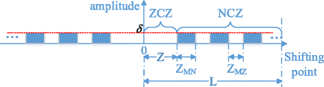

  

  Correlation properties in Theorem 1

• (p2) $Z_{\text {MN}}\leq \left (\left (m+1\right)M_{1}M^{N}+M^{N}-1 \right) - \left ({mM}_{1}M^{N}+\left (M_{1}-1\right)M^{N}\right) +1 \leq 2{M}^{N}$;

• (p3) $Z_{\text {MZ}} = L_{a}M^{N-1} - Z_{\text {MN}} \geq \left (L_{a}/M-2\right){M}^{N} = \left (M_{1}-2\right)M^{N}$;

• (p4) R _A ≤δ and R _C ≤δ.

Note that (p1), (p2), and (p3) can be directly obtained from Theorem 1; and by changing the coefficient matrix W ⁿ in step 3, the ZCZ sequence set which satisfies (p4) can be selected, where

$$\begin{aligned}</p><p class="noindent">&R_{A}=\text{max}\left\{\left|{R}_{\mathbf{a}^{N}_{i},\mathbf{a}^{N}_{j}}(\tau)\right|\right\}/E_{\mathbf{a}^{N}_{i},\mathbf{a}^{N}_{j}},\left(\tau \geq Z,i=j\right), \\ &R_{C}=\text{max}\left\{\left|{R}_{\mathbf{a}^{N}_{i},\mathbf{a}^{N}_{j}}(\tau)\right|\right\}/E_{\mathbf{a}^{N}_{i},\mathbf{a}^{N}_{j}},\left(\tau \geq Z,i\neq j\right). \end{aligned} $$

Since this factorized construction of ZCZ sequence set is an extension of existing construction based on interleaving method, here, we state the distinctive points which are different from the conventional one using the same technique. First, the interleaving construction is factorized by the matrix multiplication. This factorized formation is used widely in the construction and application of CSS [4–6, 25, 27, 28]. Note that it is the basis to deduce the efficient correlator in the next subsection. Second, since the ZCZ part is well qualified to perform CE thanks to the researches which have been done before, our works focus on the properties of NCZ part which contributes to TS: The coefficient matrix, which can be changed easily in application to generate different ZCZ sequence sets with different R _A and R _C , is added to the iteration construction; and the area with nonzero value in NCZ is determined by Theorem 1, given particular shifting PS as base ZCZ sequence set.

3.2 Efficient correlator of proposed ZCZ sequence set

Based on the proposed generation of ZCZ sequence set, an efficient correlator corresponding is derived and expressed in the following theorem.

Theorem 2.

Let $\mathbf {y}=\left [y_{0},\cdots,y_{L-1}\right ]^{\mathrm {T}}$, $\mathbf {Y}=\text {Circ}\left \{\mathbf {y},L,0\right \}$, then the efficient correlator between sequence y and each sequence $\mathbf {a}^{N}_{m},m=0,1,\cdots,M-1$, separately, is

$${} {\fontsize{8.8pt}{9.6pt}{\begin{aligned} \mathbf{Y}^{\mathrm{T}}\left[\mathbf{a}^{N}_{0},\mathbf{a}^{N}_{1},\cdots,\mathbf{a}^{N}_{M-1}\right]^{\ast}&=\mathbf{Y}^{\mathrm{T}}\left(\mathbf{A}^{N}\right)^{\ast}\\&= \mathbf{Y}^{\mathrm{T}}\left(\mathbf{A}^{0}\right)^{\ast}\!\left(\mathbf{V}^{0}\mathbf{W}^{0}\right)^{\ast}\cdots \left(\mathbf{V}^{N-1}\mathbf{W}^{N-1}\right)^{\ast} \end{aligned}}} $$

((8))

where the complexity of complex multiplication is j L L _a +N L M ² and addition is $jL\left (L_{a}-1\right)+NLM\left (M-1\right)$ in the condition that $\left \{\mathbf {a}_{m}\right \}_{m=0}^{M-1}$ are results of the circulation of j (j=1,2,⋯,M) sequences in $\left \{\mathbf {a}_{m}\right \}_{m=0}^{M-1}$.

Proof 3.

See Appendix 3. □

Table 1 illustrates the comparison of computation cost among direct correlator which computes correlation directly, radix-2 FFT corrector which converts correlation into multiplication by radix-2 FFT, the efficient correlator this paper proposed (j=1), and the correlator of the constructed ZCZ sequence set in [13]. From this table, it is obvious that the proposed efficient correlator decreases computation complexity from exponential order to linear order for iteration number N on both complex multiplication and addition, while the correlator in [13] decreases to 1/M complexity. Note that while the efficient correlator reduces large number of computation comparing with the direct correlator, it seems that there is no computational reduction speaking of the radix-2 FFT correlator. However, if we put the restrictions $\left \{a_{m,l}\right \}_{l=0}^{L_{a}-1}\in \left \{\pm 1,\pm j\right \}$, $\left \{u_{i,m}^{n}\right \}_{i=0}^{M-1}\in \left \{\pm 1,\pm j\right \}$, and $\left \{{w_{i}^{n}}\right \}_{i=0}^{M-1}\in \left \{\pm 1,\pm j\right \}$ on the generation process, then the elements in ZCZ sequence set belong to $\left \{\pm 1,\pm j\right \}$. Thus, in both the direct and the efficient correlator, there is no multiply operation, which reveals the advantage comparing to the radix-2 FFT correlator. But in [13], the alphabet size is harder to reduce to 2 or 4 even though the reduced alphabets method is used according to Section 3. So, the multiply operation cannot translate into a shifting operation. The comparison of computation cost among correlators is listed in Table 2.

Table 1 Computation complexity comparison of polyphase correlators

Table 2 Computation complexity comparison of binary/ quadriphase correlators

4 Joint MIMO TS and CE using ZCZ sequence set

In this section, we introduce how to use the ZCZ sequence as a training sequence for joint TS and CE. Using the base ZCZ sequence set $\mathcal {Z}\left (L_{a},N_{T},Z_{a}=L_{a}/N_{T}-1\right)$ which is obtained from shifting PS, the proper ZCZ sequence set $\mathcal {Z}\left (L={N_{T}}^{N}L_{a},N_{T},Z\right)=\left \{\mathbf {z}_{p}\right \}_{p=0}^{N_{T}-1}$ is generated as training sequence set, namely, s _p =z _p , which has the properties of (p1), (p2), (p3), and (p4). In order to achieve effectively the TS and CE, here, we further give two assumptions: (a1) $Z_{a}{N_{T}}^{N}+\left (N_{T}-2\right){N_{T}}^{N-1}\geq Z_{D}$; (a2) $\frac {L_{a}/N_{T}-2}{L_{a}/N_{T}}\approx 1$.

4.1 Mechanism of joint MIMO TS and CE

According to (2), it can be deduced that

$$ \mathbf{Z}^{\mathrm{H}} \mathbf{r}_{q}= \mathbf{Z}^{\mathrm{H}} \mathbf{S} \mathbf{h}_{q} +\mathbf{Z}^{\mathrm{H}} \mathbf{n}_{q}. $$

((9))

where $\mathbf {Z}=\left [\mathbf {Z}_{0},\cdots,\mathbf {Z}_{p},\cdots,\mathbf {Z}_{N_{T}-1}\right ]$, $\mathbf {Z}_{p}=\text {Circ}\left \{\mathbf {z}_{p},L,0\right \}$. Based on (a1) and (p1), it is deduced that $Z\geq Z_{a}{N_{T}}^{N}+\left (N_{T}-2\right){N_{T}}^{N-1}\geq Z_{D}$, then

$$\mathbf{Z}_{i}^{\mathrm{H}}\mathbf{S}_{j}=\left\{ \begin{aligned} E_{\mathbf{z}} \left[ \begin{array}{c} \mathbf{I}_{Z_{D}}\\ \mathbf{D}_{\mathbf{z}_{i},\mathbf{z}_{j}} \end{array} \right],i=j \\ E_{\mathbf{z}} \left[ \begin{array}{c} \mathbf{0}_{Z_{D}}\\ \mathbf{D}_{\mathbf{z}_{i},\mathbf{z}_{j}} \end{array}\right],i\neq j \end{aligned} \right., $$

then (9) can be expanded by

$${} {\fontsize{8.2pt}{9.6pt}{\begin{aligned} \mathbf{Z}_{p}^{\mathrm{H}}\mathbf{r}_{q}&=E_{\mathbf{z}} \left[ \begin{array}{ccccc} \mathbf{0}_{Z_{D}}& \cdots & \mathbf{I}_{Z_{D}} & \cdots & \mathbf{0}_{Z_{D}}\\ \mathbf{D}_{\mathbf{z}_{p},\mathbf{z}_{0}} & \cdots & \mathbf{D}_{\mathbf{z}_{p},\mathbf{z}_{p}} & \cdots & \mathbf{D}_{\mathbf{z}_{p},\mathbf{z}_{N_{T}-1}} \end{array} \right] \left[ \begin{array}{c} \mathbf{h}_{0,q} \\ \vdots \\ \mathbf{h}_{N_{T}-1,q} \end{array} \right] +\mathbf{Z}_{p}^{\mathrm{H}}\mathbf{n}_{q}\\ &=L \left[ \begin{array}{c} \mathbf{h}_{p,q}\\ \sum\limits_{i=0}^{N_{T}-1}\mathbf{D}_{\mathbf{z}_{p},\mathbf{z}_{i}}\mathbf{h}_{i,q} \end{array} \right] +\mathbf{Z}_{p}^{\mathrm{H}}\mathbf{n}_{q}, \end{aligned}}} $$

((10))

where $E_{\mathbf {z}}=E_{\mathbf {z}_{i},\mathbf {z}_{i}}=L\left (i=0,\cdots,N_{T}-1\right)$, and $\mathbf {D}_{\mathbf {z}_{p},\mathbf {z}_{i}}=\text {Circ}\left \{\mathbf {d}_{\mathbf {z}_{p},\mathbf {z}_{i}},Z_{D},0\right \}$ is a $\left (L-Z_{D}\right)\times Z_{D}$ matrix called disturbance impulse responses (DIRs), where $\mathbf {d}_{\mathbf {z}_{p},\mathbf {z}_{i}}=\left [R_{\mathbf {z}_{p},\mathbf {z}_{i}}\left (Z_{D}\right),R_{\mathbf {z}_{p},\mathbf {z}_{i}}\left (Z_{D}+1\right),\cdots,R_{\mathbf {z}_{p},\mathbf {z}_{i}}\left (L-1\right)\right ]^{\mathrm {T}}$.

By (10), the CE of h _p,q is easily obtained. In the following formula, we use (a2), (p2), (p3), and (p4) to deal with TS:

$$ \begin{aligned} \text{max}&\left\{\left|\sum\limits_{i=0}^{N_{T}-1}\mathbf{D}_{\mathbf{z}_{p},\mathbf{z}_{i}}\mathbf{h}_{i,q}\right|\right\}\leq \text{max}\left\{\sum\limits_{i=0}^{N_{T}-1}\left|\mathbf{D}_{\mathbf{z}_{p},\mathbf{z}_{i}}\mathbf{h}_{i,q}\right| \right\}\\ &\leq \delta \sum\limits_{i=0}^{N_{T}-1} \sum_{k=0}^{Z_{\text{MN}}-1}\left|{h}^{k}_{i,q}\right| \left(\mathrm{a2, p3, p4}\right) \\ &\leq 2\delta {N_{T}}^{N} \sum\limits_{i=0}^{N_{T}-1} \text{max}\left\{\left|\mathbf{h}_{i,q}\right|\right\} \left(\mathrm{p2}\right)\\ &=2\delta{N_{T}}^{N+1} \text{max}\left\{\left|\mathbf{h}_{p,q}\right|\right\}. \end{aligned} $$

((11))

According to (a2) and (p3), we have

$$ \begin{aligned} Z_{\text{MZ}}&\geq \left(L_{a}/N_{T}-2\right){N_{T}}^{N} \\ &=\frac{L_{a}/N_{T}-2}{L_{a}/N_{T}}L_{a}{N_{T}}^{N-1}\\ &>\frac{L_{a}/N_{T}-2}{L_{a}/N_{T}}Z \left(\text{bound in \cite{2000XiaohuTang}}\right)\\ &\geq \frac{L_{a}/N_{T}-2}{L_{a}/N_{T}}Z_{D}\approx Z_{D}. \end{aligned} $$

((12))

Thus, the second inequality of (11) is deduced; and the last equation of (11) is achieved by the requirement which is

$${} \text{max}\left\{\left|\mathbf{h}_{i,q}\right|\right\}=\text{max}\left\{\left|\mathbf{h}_{p,q}\right|\right\},i=0,1,\cdots,N_{T}-1. $$

((13))

If

$$ \delta\leq 1/\left(2{N_{T}}^{N+1}\right), $$

((14))

then

$$ \text{max}\left\{\left|\sum_{i=0}^{N_{T}-1}\mathbf{D}_{\mathbf{z}_{p},\mathbf{z}_{i}}\mathbf{h}_{i,q}\right|\right\}\leq \text{max}\left\{\left|\mathbf{h}_{p,q}\right|\right\}. $$

((15))

Using this, we can achieve TS by looking for the maximum value in $\left |\mathbf {Z}_{p}^{\mathrm {H}}\mathbf {r}_{q}\right |$. This mechanism is illustrated in Fig. 2. Note that the impulse responses which represent complex value are described in the form of absolute value in the figure.

Fig. 2

Joint TS and CE

However, in practice, because of the randomness of the MIMO channel, the energy of h _i,q , i≠p can be larger than that of h _p,q , which is called energy interference among channels. Thus, in that case, (13) is substituted by

$${} \text{max}\left\{\left|\mathbf{h}_{i,q}\right|\right\}>\text{max}\left\{\left|\mathbf{h}_{p,q}\right|\right\},\left(i\neq p,i=0,1,\cdots,N_{T}-1\right)\!. $$

Then, (15) could be changed by

$$\text{max}\left\{\left|\sum_{i=0}^{N_{T}-1}\mathbf{D}_{\mathbf{z}_{p},\mathbf{z}_{i}}\mathbf{h}_{i,q}\right|\right\}>\text{max}\left\{\left|\mathbf{h}_{p,q}\right|\right\}. $$

So, it is infeasible to rely on $\mathbf {Z}_{p}^{\mathrm {H}}\mathbf {r}_{q}$ to perform TS. The energy interference among channels is illustrated in Fig. 3.

Fig. 3

Energy interference among channels

4.2 Solutions of the energy interference among channels

To deal with the energy interference among channels for TS, the direct way, called solution 1, is only considering the largest energy of CIR such as h _i,q and discarding all the others which may be submerged by DIRs such as h _p,q , as illustrated in Fig. 3. Solution 1 is indicated by

$$ \text{max}\left\{\text{max}\left\{\left|\mathbf{Z}_{p'}^{\mathrm{H}}\mathbf{r}_{q}\right|\right\}\right\}_{p'=0}^{N_{T}-1}. $$

((16))

When the energy interference among channels is severe, just in the case like Fig. 3, (16) works well. However, when that interference is mild, meaning that energies of all channels are similar, (16) loses nearly $\left (N_{T}-1\right)/N_{T}$ information which is useful for TS. This deficiency of (16) makes the performance of TS decline.

To perform TS better in the situations that the energy interference among channels are both severe and mild, an easier way is taking account of all the correlation results in $\left \{\mathbf {Z}_{p}^{\mathrm {H}}\mathbf {r}_{q}\right \}_{p=0}^{N_{T}-1}$ jointly. This idea is indicated by (17).

$${} \sum_{p=0}^{N_{T}-1}\left|\mathbf{Z}_{p}^{\mathrm{H}}\mathbf{r}_{q}\right|=L \left[ \begin{array}{c} \sum\limits_{p=0}^{N_{T}-1}\left|\mathbf{h}_{p,q}\right|\\ \sum\limits_{p=0}^{N_{T}-1}\left|\sum\limits_{i=0}^{N_{T}-1}\mathbf{D}_{\mathbf{z}_{p},\mathbf{z}_{i}}\mathbf{h}_{i,q}\right| \end{array} \right] +\sum_{p=0}^{N_{T}-1}\left|\mathbf{Z}_{p}^{\mathrm{H}}\mathbf{n}_{q}\right|. $$

((17))

Similar to (11), it is deduced that

$$ \begin{aligned} &\text{max}\left\{\left|\sum\limits_{p=0}^{N_{T}-1}\left|\sum\limits_{i=0}^{N_{T}-1}\mathbf{D}_{\mathbf{z}_{p},\mathbf{z}_{i}}\mathbf{h}_{i,q}\right|\right|\right\}\\ \leq &\text{max}\left\{\sum\limits_{p=0}^{N_{T}-1}\sum\limits_{i=0}^{N_{T}-1}\left|\mathbf{D}_{\mathbf{z}_{p},\mathbf{z}_{i}}\mathbf{h}_{i,q}\right| \right\}\\ \leq& \delta N_{T} \sum\limits_{i=0}^{N_{T}-1} \sum_{k=0}^{Z_{\text{MZ}}-1}\left|{h}^{k}_{i,q}\right| \\ \leq& 2\delta {N_{T}}^{N+1} \sum\limits_{i=0}^{N_{T}-1} \text{max}\left\{\left|\mathbf{h}_{i,q}\right|\right\}. \end{aligned} $$

((18))

If it is satisfied that

$$ \text{max}\left\{\sum_{p=0}^{N_{T}-1}\left|\mathbf{h}_{p,q}\right|\right\}=\sum_{i=0}^{N_{T}-1} \text{max}\left\{\left|\mathbf{h}_{i,q}\right|\right\}, $$

((19))

then based on (14) and (18),

$$\text{max}\left\{\sum\limits_{p=0}^{N_{T}-1}\left|\sum\limits_{i=0}^{N_{T}-1}\mathbf{D}_{\mathbf{z}_{p},\mathbf{z}_{i}}\mathbf{h}_{i,q}\right|\right\}\leq \text{max}\left\{\sum\limits_{p=0}^{N_{T}-1}\left|\mathbf{h}_{p,q}\right|\right\}. $$

TS can be achieved by looking for the maximum absolute value in $\sum _{p=0}^{N_{T}-1}\left |\mathbf {Z}_{p}^{\mathrm {H}}\mathbf {r}_{q}\right |$ without considering (13); and it is presented in Fig. 4 vividly.

Fig. 4

Correlations summing solution of energy interference among channels

But in some cases, and they are not quite rare, the condition in (19) which needs to be fulfilled cannot be achieved. Note that the position of maximum of $\left |\mathbf {h}_{i,q}\right |$ is different from that of $\left |\mathbf {h}_{p,q}\right |$ to a large extent because of randomness of MIMO channel (i≠p); and even worse, the position of maximum of $\left |\mathbf {h}_{i,q}\right |$ may be corresponding to the position of a very small value of $\left |\mathbf {h}_{p,q}\right |$. In that case, the risk that CIRs are overwhelmed by DIRs is much higher. This bug is shown in Fig. 5.

Fig. 5

The bug of correlations summing solution

To fix the bug, the maximum of each $\left |\mathbf {h}_{p,q}\right |$, p=0,⋯,N _T −1 should be selected to add together to get $\sum _{i=0}^{N_{T}-1} \text {max}\left \{\left |\mathbf {h}_{i,q}\right |\right \}$ according to (18). To achieve this goal, $\left |\mathbf {Z}_{p}^{\mathrm {H}}\mathbf {r}_{q}\right |$ is grouped into N _X parts successively indicated by $\mathbf {c}_{p,q}^{n'}\phantom {\dot {i}\!}$, and the length of the each group is $l^{n'}\phantom {\dot {i}\!}$, n ^′=0,⋯,N _X −1. Then, find the value of (20) to perform TS for qth receiving antenna.

$$ \text{max}\left\{\sum_{p=0}^{N_{T}-1}\left\{\text{max}\left\{\left|\mathbf{c}_{p,q}^{n'}\right|\right\}_{n'=0}^{N_{X}-1}\right\} \right\} $$

((20))

To let (20) make sense in application, it needs to make sure the maximum of $\left \{\left |\mathbf {h}_{p,q}\right |\right \}_{p=0}^{N_{T}-1}\phantom {\dot {i}\!}$ be grouped to one group. First, $l^{n'}\phantom {\dot {i}\!}$ satisfies $l^{n'}\geq 2M_{P}\phantom {\dot {i}\!}$ with restriction lower better to avoid the bug, where M _P <Z _D is the maximum distance between positions of the maximum value of $\left \{\left |\mathbf {h}_{p,q}\right |\right \}_{p=0}^{N_{T}-1}\phantom {\dot {i}\!}$. Thus, $l^{n'}=2M_{P}\phantom {\dot {i}\!}$ or $l^{n'}=2M_{P}+1\phantom {\dot {i}\!}$. Second, it groups $\left |\mathbf {Z}_{p}^{\mathrm {H}}\mathbf {r}_{q}\right |$ two times to get two different sets of groups by starting from two different start points S _p1 and S _p2, where $\left |S_{p1}-S_{p2}\right |=M_{P}$. By doing so, it is guaranteed that the maximum of $\left \{\left |\mathbf {h}_{p,q}\right |\right \}_{p=0}^{N_{T}-1}\phantom {\dot {i}\!}$ be grouped in one of the two sets of groups. The process called solution 2 is demonstrated in Fig. 6.

Fig. 6

Solution 2 of energy interference among channels

Taking advantage of the idea of solution 2, we propose an algorithm called twice section-maximum algorithm to perform TS and CE jointly. In the following algorithm, we use $\mathcal {C}\left \{\mathbf {r}_{q},\mathcal {Z}\left (L,N_{T},Z\right)\right \}$ to denote the correlation operation between column vector r _q and N _T ZCZ sequences in the set $\mathcal {Z}\left (L,N_{T},Z\right)$ utilizing the efficient correlator obtained from Theorem 2.

5 Simulations

5.1 Communication scenario setting

To evaluate the performance of joint TS and CE using constructed ZCZ sequence set, numerical simulations are performed in millimeter wave (mmWave) channel [31] and channel model D of 802.11 ac [32] based on the SC-MIMO-FDE system. We assume 4 transmitting antennas and 4 receiving antennas to transmit 4 spacial data streams, and the number of transmit frame is 10,000. For mmWave channel, the small-scale MIMO channel fading model is a virtual model with 25 paths obtained by the timing overlap of the Saleh-Velenzuela (SV) model, the carrier frequency is set to be F _C =45 GHz in mmWave band, the chip rate is F _S =440 MHz, and the maximum multi-path time delay is T _M =100 ns. For channel model D of 802.11 ac, there are 18 channel paths. The carrier frequency is F _C =5.25 GHz, the chip rate is F _S =12.5 MHz, and the maximum multi-path time delay is T _M =400 ns. These parameters are summarized in Table 3.

Table 3 Simulation parameters

5.2 ZCZ sequence set selection

Since there are 4 transmitting antennas, and Z _D =T _M F _S ≤50, we construct a ZCZ quadriphase sequence set $\mathcal {Z}\left (256,4,56\right)$ based on Theorem 1, where Z=56>Z _D , Z _MN=22≤32, and Z _MZ=38≥32. When searching for the proper ZCZ sequence set, the restrictions of R _A <δ and R _C <δ are considered. By randomly changing coefficient matrix W ⁿ using the efficient generator, a ZCZ sequence set with δ=0.3 is found. While theoretical restriction in (14) is $\delta \leq 1/2{N_{T}}^{N+1}=1/128$ and more precise restriction in (18) is $\delta \leq 1/\left (Z_{\text {MN}}N_{T}\right)=1/88$, both of which seem unapproachable, but considering the fading and the random distribution of phase of CIR taps in the real communication system, δ is allowed to be much larger than the restriction, and practically the performance of δ=0.3 is excellent in the simulation. The generation parameters are listed as the following:

• (1) Base ZCZ sequence set is $\mathcal {A}=\left \{\mathbf {a}_{m}\right \}_{m=0}^{3}$, where $\mathbf {a}_{m}=\text {Circ}\left \{\mathbf {a},1,-4m\right \}$, and $\mathbf {a}=\left [1,1,1,1,1,j,-1,-j,1,-1,1,-1,1,-j,-1,j \right ]^{\mathrm {T}}$ is a PS.

• (2) Number of iterations is N=2.

• (3) U ⁰ and U ¹ are

  $$\mathbf{U}^{0}= \left[ \begin{array}{cccc} 1& 1& 1& 1 \\ 1& -1 &1 &-1 \\ 1& 1& -1 &-1 \\ 1 &-1 &-1 &1 \end{array} \right]; \mathbf{U}^{0}= \left[ \begin{array}{cccc} 1& 1& 1& 1 \\ 1& j &-1 &-j \\ 1& -1& 1 &-1 \\ 1 &-j &-1 &j \end{array} \right]. $$

• (4) Coefficients ${w_{m}^{n}}$ (m=0,1,2,3; n=0,1) are

  $$\left[ \begin{array}{cc} {w_{0}^{0}}& {w_{0}^{1}} \\ {w_{1}^{0}}& {w_{1}^{1}}\\ {w_{2}^{0}} & {w_{2}^{1}} \\ {w_{3}^{0}} &{w_{3}^{1}} \end{array} \right] = \left[ \begin{array}{cc} -1& -1 \\ -1& -1\\ j & j \\ -j &-j \end{array} \right]. $$

The autocorrelation and cross-correlation results with the largest R _A and R _C are shown in Figs. 7 and 8, respectively. For the detail of $\mathcal {Z}\left (256,4,56\right)$, see Table 4, where 0,1,2,3 represent 1,j,−1,−j.

Fig. 7

Normalized autocorrelation of ZCZ sequence set with maximum side lobes

Fig. 8

Normalized cross-correlation of ZCZ sequence set with maximum side lobes

Table 4 ZCZ sequence set

5.3 Performance and computational complexity analysis

In this section, we compare our works with Wang’s method [33] mainly. We use the ZC sequence with the length of 256 as MIMO training sequence in Wang’s method. And the length of CP is set to be 50≥Z _D , which satisfies the demand of Wang’s method. The training sequence transmitting arrangement of Wang’s method and this paper’s method are described in Fig. 9. According to this figure, our method cost almost as half as the preamble consumption of Wang’s method.

Fig. 9

Training sequence transmitting arrangement

Figures 10 and 11 show the precise rate of the three methods mentioned to deal with TS. Note that there exists CP=64 in front of each data block; it is feasible to put a start position in the range of CP tolerance called R, which is R=CP−T _M F _S . Suppose that the true symbol beginning position is P _T , then we treat it as a correct TS if $-R\leq \hat {P}_{q}^{n'_{0}}-P_{T}\leq 0$. It is clear that accuracy of solution 1 is degraded by overlooking approximately $\left (N_{T}-1\right)/N_{T}$ channel information. Solution 2 has an excellent performance in both the lower SNR area and higher SNR area. While the Wang’s method performs pretty good in the higher SNR area, it degrades badly in the lower SNR area. The reason is that it needs coarse TS before accurate TS, and the coarse TS uses slide correlation method, which is more sensitive to noise disturbance.

Fig. 10

Performance of TS (channel model D of 802.11ac)

Fig. 11

Performance of TS (mmWave channel)

Figure 12 shows the normalized mean square error (NMSE) performance of CE using the LS estimator. In the simulation, MIMO channels are normalized by $\frac {1}{N_{T}N_{R}}\sum _{q=0}^{N_{R}-1}\mathbf {h}_{q}^{\mathrm {H}}\mathbf {h}_{q}=1$. Based on (4), the CRLB of NMSE is

$${} {\fontsize{9.2pt}{9.6pt}{\begin{aligned} \mathrm{{NMSE}_{CRLB}}&=\text{MSE}/\mathrm{E}\left\{h_{p,q}^{i}\right\}\\ &=\frac{\sigma^{2}}{N_{T}Z_{D}}\text{tr}\left\{\left(\mathbf{S}^{\mathrm{H}} \mathbf{S} \right)^{-1} \right\}/\left(\frac{1}{Z_{D}N_{T}N_{R}}\sum_{q=0}^{N_{R}-1}\mathbf{h}_{q}^{\mathrm{H}}\mathbf{h}_{q}\right)\\ &=\frac{\sigma^{2}Z_{D}}{{\sigma_{D}^{2}}L}=\frac{\sigma^{2}N_{T}Z_{D}}{L}, \end{aligned}}} $$

((21))

Fig. 12

Performance of CE

where ${\sigma _{D}^{2}}$ is the energy of transmitting signal, and it is normalized by $N_{T}{\sigma _{D}^{2}}=1$, so the last equation in (21) is demonstrated; and the NMSE of CE is $\mathrm {{NMSE}_{\textit {CE}}}=\mathrm {E}\left \{\sum _{q=0}^{N_{R}-1}\hat {\mathbf {h}}_{q}^{\mathrm {H}}\hat {\mathbf {h}}_{q}\right \}/\mathrm {E}\left \{\sum _{q=0}^{N_{R}-1}\mathbf {h}_{q}^{\mathrm {H}}\mathbf {h}_{q}\right \}$. It indicates that both of the CE methods attain CRLB.

Table 5 gives a joint TS and CE computational cost comparison between the twice section-maximum algorithm and Wang’s method. In this simulation, L=256, N _R =N _T =4, N _X =8, L _a =16, N=2, Z _D =50, so the addition complexity of twice section-maximum algorithm is about 4×256×41, while Wang’s method 4×256×265; Since the elements of $\mathcal {Z}\left (256,4,56\right)$ are quadriphase, the complex multiplication in twice section-maximum algorithm is substituted by shifting operation, which is much faster than multiplication, while it is about 4×256×259. Overall, it is generalized that the twice section-maximum algorithm is more computational efficient.

Table 5 Computational cost comparison between joint TS and CE methods

6 Conclusions

A factorized construction of ZCZ sequence set with the efficient generator and correlator has been investigated and applied to TS and CE jointly for the SC-MIMO-FDE system. Considering the properties of ZCZ and NCZ, the efficient generator can generate ZCZ sequence set suitable for CE and TS simultaneously. Further, the twice section-maximum algorithm is proposed and behaves well to eliminate the energy interference among channels; and the efficient correlator reduces complex multiplication, which can be avoided for efficient quadriphase or binary correlator, and complex addition from exponential order to linear order. Both efficient correlator and mechanism of joint TS and CE can reduce the processing time for the receiver.

7 Appendix 1

Proof of Lemma 1

Let the shifting matrix be $\mathbf {T}_{l}=\text {Circ}\left \{\mathbf {e}_{L},L,l\right \}$, $l=0,\pm 1,\cdots,\pm \left (L-1\right)$, where e _L is a unite vector of the size L×1 with the first entry equal to 1. The base ZCZ sequence set $\mathcal {A}$ satisfies

$$ {R}_{\mathbf{a}_{i},\mathbf{a}_{j}}(\tau) =\left\{ \begin{aligned} E_{\mathbf{a}_{i},\mathbf{a}_{j}},\left(\tau=0, i=j\right)\\0, \left(0 < \left|\tau\right| \leq Z_{a}, i =j\right) \\ 0,\left(0 \leq \left|\tau\right| \leq Z_{a}, i \neq j\right) \end{aligned} \right.. $$

((22))

So, $\left (\mathbf {T}_{l}\mathbf {A}^{N} \right)^{\mathrm {H}}\mathbf {A}^{N}=$

$$\left(\mathbf{V}^{N-1}\mathbf{W}^{N-1}\right)^{\mathrm{H}}\cdots \left(\mathbf{T}_{l}\mathbf{A}^{0} \right)^{\mathrm{H}} \mathbf{A}^{0}\mathbf{V}^{0}\mathbf{W}^{0}\cdots \mathbf{V}^{N-1}\mathbf{W}^{N-1} $$

satisfies the two situations using (22):

• ■ (a) $\left |l\right | \leq M^{N}Z_{a}$

  $$\left(\mathbf{T}_{l}\mathbf{A}^{0} \right)^{\mathrm{H}}\mathbf{A}^{0} =\left\{ \begin{aligned} &\hat{\mathbf{R}}_{l}&,&\left|l\right|\leq M^{N-1}-1 \\ &\mathbf{0}_{M^{N}}&,& M^{N-1}\leq \left|l\right| \leq M^{N}Z_{a} \end{aligned} \right., $$

  where $\hat {\mathbf {R}}_{l}=\text {diag}_{l}\left \{E_{\mathbf {a}_{0}}\mathbf {R}_{l},E_{\mathbf {a}_{1}}\mathbf {R}_{l},\cdots,E_{\mathbf {a}_{M-1}}\mathbf {R}_{l}\right \}$ with the size of M ^N×M ^N, and $\mathbf {R}_{l}=\text {diag}_{l}\left \{1,1,\cdots,1\right \}$ with the size of M ^N−1 × M ^N−1. When $\left |l\right |\!\leq \! M^{N-1}\,-\,1$, $\left (\mathbf {T}_{l}\mathbf {A}^{N} \right)^{\mathrm {H}}\mathbf {A}^{N}=$

  $$\begin{aligned} &\left(\mathbf{V}^{N-1}\mathbf{W}^{N-1}\right)^{\mathrm{H}}\cdots\left(\mathbf{V}^{1}\mathbf{W}^{1}\right)^{\mathrm{H}} \hat{\mathbf{R}}_{l} \mathbf{V}^{0}\mathbf{W}^{0}\cdots \mathbf{V}^{N-1}\mathbf{W}^{N-1}\\ &=\left\{ \begin{aligned} &\mathbf{I}_{M}&,&l=0\\&\mathbf{0}_{M}&,&1\leq\left|l\right|\leq M^{N-1}-1 \end{aligned} \right.; \end{aligned} $$

  When $\left |l\right | \geq M^{N-1}$, $\left (\mathbf {T}_{l}\mathbf {A}^{N} \right)^{\mathrm {H}}\mathbf {A}^{N}=\mathbf {0}_{M}$.

• ■ (b) $\left |l\right |= M^{N}Z_{a}+1$

  $$ \left(\mathbf{T}_{l}\mathbf{A}^{0} \right)^{\mathrm{H}}\mathbf{A}^{0}\,=\,\left\{\!\! \begin{aligned} &\text{diag}_{1-M^{N}}\left\{R_{\mathbf{a}_{M-1},\mathbf{a}_{0}}\left(Z_{a}+1\right)\right\},l>0\\ &\text{diag}_{M^{N}-1}\left\{R_{\mathbf{a}_{0},\mathbf{a}_{M-1}}\left(-Z_{a}-1\right)\right\},l<0 \end{aligned} \right.. $$

  If the length of ZCZ between a _M−1 and a ₀ is Z _a , then $R_{\mathbf {a}_{M-1},\mathbf {a}_{0}}\left (Z_{a}+1\right)=R_{\mathbf {a}_{0},\mathbf {a}_{M-1}}\left (-Z_{a}-1\right)\neq 0$, so $\left (\mathbf {T}_{l}\mathbf {A}^{N} \right)^{\mathrm {H}}\mathbf {A}^{N}\neq \mathbf {0}_{M}$. Otherwise, the length of ZCZ between a _M−1 and a ₀ is larger than Z _a , then $R_{\mathbf {a}_{M-1},\mathbf {a}_{0}}\left (Z_{a}+1\right)=R_{\mathbf {a}_{0},\mathbf {a}_{M-1}}\left (-Z_{a}-1\right)= 0$, so $\left (\mathbf {T}_{l}\mathbf {A}^{N} \right)^{\mathrm {H}}\mathbf {A}^{N}= \mathbf {0}_{M}$.

  Combining (a) and (b), we can obtain the conclusion: If the length of ZCZ between a _M−1 and a ₀ is Z _a , then Z=M ^N Z _a ; Otherwise, Z>M ^N Z _a .

8 Appendix 2

Proof of Theorem 1

Based on the definition of PS, it is easy to deduce that

$${} {R}_{\mathbf{a}_{i},\mathbf{a}_{j}}(\tau) =\left\{ \begin{aligned} E_{\mathbf{a}}&,& \left(\text{mod}\left\{\tau,{MM}_{1}\right\}=\left(i-j\right)M_{1}, i \neq j\right) \\ 0&,&\left(\text{others}\right) \end{aligned} \right.. $$

((23))

• ■ (a) First, we prove $Z\geq \left (M_{1}-1\right)M^{N}+\left (M-2\right) M^{N-1}$.

• ■ (a. 1) $N=1\left (\mathbf {T}_{l}\mathbf {A}^{N} \right)^{\mathrm {H}}\mathbf {A}^{N}=\left (\mathbf {V}^{0}\mathbf {W}^{0}\right)^{\mathrm {H}}\left (\mathbf {T}_{l}\mathbf {A}^{0} \right)^{\mathrm {H}} \mathbf {A}^{0}\mathbf {V}^{0}\mathbf {W}^{0}$ satisfies the two situations:

• ■ (a. 1. 1) $\left |l\right | \leq \left (M_{1}-1\right)M$

  The proof is the same as case (a) in Appendix 1.

• ■ (a. 1. 2) $\left (M_{1}-1\right)M+1\leq \left |l\right | \leq \left (M_{1}-1\right)M+M-2 \left (\mathbf {T}_{l}\mathbf {A}^{0} \right)^{\mathrm {H}}\mathbf {A}^{0}=$

  $${} \left\{\begin{aligned} \text{diag}_{l-M_{1}M}&\left\{R_{\mathbf{a}_{M_{1}M-l},\mathbf{a}_{0}}\left(M_{1}\right),R_{\mathbf{a}_{M_{1}M-l+1},\mathbf{a}_{1}}\left(M_{1}\right),\right.&\\ & \left. \cdots,R_{\mathbf{a}_{M-l},\mathbf{a}_{l-\left(M_{1}-1\right)M-1}}\left(M_{1}\right) \right\},l>0&\\ \text{diag}_{l+M_{1}M}&\left\{R_{\mathbf{a}_{0},\mathbf{a}_{M_{1}M+l}}\left(-M_{1}\right),R_{\mathbf{a}_{1},\mathbf{a}_{M_{1}M+l+1}}\left(-M_{1}\right), \right.&\\ & \left.\cdots,R_{\mathbf{a}_{-l-\left(M_{1}-1\right)M-1},\mathbf{a}_{M-l}}\left(-M_{1}\right) \right\},l<0 & \end{aligned} \right.. $$

From (23), it is known that

$$ {R}_{\mathbf{a}_{i},\mathbf{a}_{j}}\left(M_{1} \right) =\left\{ \begin{aligned} E_{\mathbf{a}}&,&\left(i=j+1\right) \\ 0&,&\left(\text{others}\right) \end{aligned} \right., $$

((24))

and

$$ {R}_{\mathbf{a}_{i},\mathbf{a}_{j}}\left(-M_{1} \right) =\left\{ \begin{aligned} E_{\mathbf{a}}&,&\left(j=i+1\right) \\ 0&,&\left(\text{others}\right) \end{aligned} \right.. $$

((25))

So, $R_{\mathbf {a}_{M_{1}M-\left |l\right |+k},\mathbf {a}_{k}}\left (M_{1}\right)=0$ and $R_{\mathbf {a}_{k},\mathbf {a}_{M_{1}M-\left |l\right |+k}}\left (-M_{1}\right)=0$, $k=0,1,\cdots,\left |l\right |-\left (M_{1}-1\right)M-1$. Then, $\left (\mathbf {T}_{l}\mathbf {A}^{0} \right)^{\mathrm {H}}\mathbf {A}^{0}=\mathbf {0}_{M}$, and $\left (\mathbf {T}_{l}\mathbf {A}^{N} \right)^{\mathrm {H}}\mathbf {A}^{N}=\mathbf {0}_{M}$.

Combining (a. 1. 1) and (a. 1. 2), it is obtained that $Z\geq \left (M_{1}-1\right)M+\left (M-2\right)$.

• ■ (a. 2) N>1

  Using the ZCZ sequence set generated in (a. 1), we can easily get $Z\geq \left (M_{1}-1\right)M^{N}+\left (M-2\right)M^{N-1}$ according to Lemma 1.

  Combining (a. 1) and (a. 2), $Z\geq \left (M_{1}-1\right)M^{N}+\left (M-2\right)M^{N-1}$ is proved.

• ■ (b) Now, we prove both the autocorrelation and cross-correlation have $Z_{N}\leq 4\left (M-1\right)M^{N}$ nonzero values.

• ■ (b. 1) When ${mM}_{1}M^{N}+M^{N}\leq \left |l\right |\leq {mM}_{1}M^{N}+ \left (M_{1}-1\right)M^{N}-1$, $\left (\mathbf {T}_{l}\mathbf {A}^{0} \right)^{\mathrm {H}}\mathbf {A}^{0}=\mathbf {0}_{M}$ is deduced based on (23), where m=0,1,⋯,M−1. Thus, $\left (\mathbf {T}_{l}\mathbf {A}^{N} \right)^{\mathrm {H}}\mathbf {A}^{N}=\mathbf {0}_{M}$.

• ■ (b. 2) When $0<\left |l\right |<M^{N}$, $\left (\mathbf {T}_{l}\mathbf {A}^{N} \right)^{\mathrm {H}}\mathbf {A}^{N}=\mathbf {0}_{M}$ according to case (a) in Appendix 1.

  Except case (b. 1) and (b. 2) where ZCZ across whole correlation, the area with nonzero value is bounded by ${mM}_{1}M^{N}+\left (M_{1}-1\right)M^{N}\leq \left |l\right |\leq \left (m+1\right)M_{1}M^{N} +M^{N}-1$, m=0,1,⋯,M−2.

9 Appendix 3

Proof of Theorem 2

The efficient correlator can be easily obtained by

$$\begin{aligned} \mathbf{Y}^{\mathrm{T}}\left(\mathbf{A}^{N}\right)^{\ast}&=\mathbf{Y}^{\mathrm{T}} \left(\mathbf{A}^{0}\mathbf{V}^{0}\mathbf{W}^{0}\mathbf{V}^{1}\mathbf{W}^{1}\cdots \mathbf{V}^{N-1}\mathbf{W}^{N-1}\right)^{\ast}\\ &=\mathbf{Y}^{\mathrm{T}}\left(\mathbf{A}^{0}\right)^{\ast}\left(\mathbf{V}^{0}\mathbf{W}^{0}\right)^{\ast}\cdots \left(\mathbf{V}^{N-1}\mathbf{W}^{N-1}\right)^{\ast}. \end{aligned} $$

Next, we analyze computational complexity of the correlator step by step.

• ■ (a) Computational complexity of A ⁰:

  Let $\mathbf {Y}^{\mathrm {T}}\left (\mathbf {a}^{0}_{m}\right)^{*}=\mathbf {g}_{m}^{0}$, then

  $$ \mathbf{Y}^{\mathrm{T}}\left(\mathbf{A}^{0}\right)^{\ast}=\mathbf{G}^{0}=\left[\mathbf{G}_{0}^{0},\cdots,\mathbf{G}_{m}^{0},\cdots,\mathbf{G}_{M-1}^{0}\right], $$

  where $\mathbf {G}_{m}^{0}=\text {Circ}\left \{\mathbf {g}_{m}^{0},M^{N-1},mM^{N-1}\right \}$. So, only $\mathbf {g}_{m}^{0}$ is needed to construct $\mathbf {g}_{m}^{0}$; and it takes L M L _a complex multiplication and $LM\left (L_{a}-1\right)$ complex addition. In general, if $\left \{\mathbf {a}_{m}\right \}_{m=0}^{M-1}$ are results of the circulation of j (j=1,2,⋯,M) sequences in $\left \{\mathbf {a}_{m}\right \}_{m=0}^{M-1}$, $\left \{\mathbf {a}_{m}^{0}\right \}_{m=0}^{M-1}$ are results of the circulation of j sequences in $\left \{\mathbf {a}_{m}^{0}\right \}_{m=0}^{M-1}$, too. Thus, j sequences in $\left \{\mathbf {g}_{m}^{0}\right \}_{m=0}^{M-1}$ are needed to construct $\left \{\mathbf {g}_{m}^{0}\right \}_{m=0}^{M-1}$; and it takes j L L _a complex multiplication and $jL\left (L_{a}-1\right)$ complex addition.

• ■ (b) Computational complexity of V ⁱ W ⁱ (0≤i≤N−2):

  Let $\mathbf {G}^{i+1}=\mathbf {G}^{i}\left (\mathbf {V}^{i}\mathbf {W}^{i}\right)^{*}$. If

  $$ \mathbf{G}^{i}=\left[\mathbf{G}_{0}^{i},\cdots,\mathbf{G}_{m}^{i},\cdots,\mathbf{G}_{M-1}^{i}\right], $$

  where $\mathbf {G}_{m}^{i}=\text {Circ}\left \{\mathbf {g}_{m}^{i},M^{N-1-i},mM^{N-1-i}\right \}$. Then,

  $$ \mathbf{G}^{i+1}=\left[\mathbf{G}_{0}^{i+1},\cdots,\mathbf{G}_{m}^{i+1},\cdots,\mathbf{G}_{M-1}^{i+1}\right], $$

  where $\mathbf {G}_{m}^{i+1}=\text {Circ}\left \{\mathbf {g}_{m}^{i+1},M^{N-2-i},mM^{N-2-i}\right \}$. So, only $\mathbf {g}_{m}^{i+1}$ is needed to construct $\mathbf {g}_{m}^{i+1}$; and it takes L M ² complex multiplication and $LM\left (M-1\right)$ complex addition.

• ■ (c) Computational complexity of V ^N−1 W ^N−1:

  Since V ^N−1 W ^N−1 is a matrix with the size M×M and G ^N−1 is a matrix L×M, it is easy to see that $\mathbf {G}^{N}=\mathbf {G}^{N-1}\left (\mathbf {V}^{N-1}\mathbf {W}^{N-1}\right)^{*}$ takes L M ² complex multiplication and $LM\left (M-1\right)$ complex addition.

  Combining (a), (b), and (c), we can obtain the conclusion: The efficient correlator takes j L L _a +N L M ² complex multiplication and $jL\left (L_{a}-1\right)+NLM\left (M-1\right)$ complex addition in the condition that $\left \{\mathbf {a}_{m}\right \}_{m=0}^{M-1}$ are results of the circulation of j sequences in $\left \{\mathbf {a}_{m}\right \}_{m=0}^{M-1}$.

References

D Falconer, SL Ariyavisitakul, A Benyamin-Seeyar, B Eidson, Frequency domain equalization for single-carrier broadband wireless systems. IEEE Commun. Mag.40(4), 58–66 (2002).
AJ Paulraj, DA GORE, RU Nabar, H Bolcskei, An overview of MIMO communications—a key to gigabit wireless. Proc. IEEE.92(2), 198–218 (2004).
SQ Wang, A Abdi, Low-complexity optimal estimation of MIMO ISI channels with binary training sequences. IEEE Signal Proc. Lett.13(11), 657–660 (2006).
HM Wang, XQ Gao, B Jiang, XH You, W Hong, Efficient MIMO channel estimation using complementary sequences. IET Commun.1(5), 962–969 (2007).
HM Wang, XQ Gao, B Jiang, W Hong, Improved channel estimator for MIMO-SCBT systems using quadriphase complementary sequences. IEICE Trans. Commun.94:, 342–345 (2011).
HM Wang, Efficient generator and correlator for MOPCSSs and their application to MIMO channel estimation. IEICE ComEX.1:, 16–22 (2012).
XQ Gao, B Jiang, XH You, ZW Pan, YS Xue, E Schulz, Efficient channel estimation for MIMO single-carrier block transmission with dual cyclic timeslot structure. IEEE Trans. Commun.55(11), 2210–2223 (2007).
PZ Fan, N Suehiro, N Kuroyanagi, XM Deng, Class of binary sequences with zero correlation zone. Electron. Lett.35(10), 777–779 (1999).
PZ Fan, Spreading sequence design and theoretical limits for quasisynchronous CDMA systems. EURASIP J. Wirel. Commun. Netw.1:, 19–31 (2004).
SA Yang, JS Wu, Optimal binary training sequence design for multiple-antenna systems over dispersive fading channels. IEEE Trans. Veh. Technol.51(5), 1271–1276 (2002).
PZ Fan, WH Mow, On optimal training sequence design for multiple-antenna systems over dispersive fading channels and its extensions. IEEE Trans. Veh. Technol.53(5), 1623–1626 (2004).
R Zhang, X Cheng, M Ma, B Jiao, Interference-avoidance pilot design using ZCZ sequences for multicell MIMOOFDM systems. Global Communications Conference (GLOBECOM), 3-7 December 2012, Anaheim, California:5056–5061.
BM Popovic, O Mauritz, Generalized chirp-like sequences with zero correlation zone. IEEE Trans. Inf. Theory.56(6), 2957–2960 (2010).
YC Liu, CW Chen, YT Su, New constructions of zero-correlation zone sequences. IEEE Trans. Inf. Theory.59(8), 4994–5007 (2013).
R Appuswamy, AK Chaturvedi, 52. IEEE Trans. Inf. Theory.8:, 3817–3826 (2006).
CG Han, TS Hashimoto, N Suehiro, A new construction method of zero-correlation zone sequences based on complete complementary codes. IEICE Trans. Fundam. Electron. Commun. Comput. Sci.E91-A(12), 3698–3702 (2008).
CC Tseng, C Liu, Complementary sets of sequences. IEEE Trans. Inf. Theory.18(5), 644–6552 (1972).
H Torii, M Nakamura, N Suehiro, A new class of zero-correlation zone sequences. IEEE Trans. Inf. Theory.50(3), 559–565 (2004).
HG Hu, G Gong, New sets of zero or low correlation zone sequences via interleaving techniques. IEEE Trans. Inf. Theory.56(4), 1702–1713 (2010).
PZ Fan, M Darnell, The synthesis of perfect sequences. Cryptography and coding (Springer, Berlin, 1995).
XH Tang, PZ Fan, S Matsufuji, Lower bounds on correlation of spreading sequence set with low or zero correlation zone. Electron. Lett.36(6), 551–552 (2000).
SZ Budisin, Efficient pulse compressor for Golay complementary sequences. Electron. Lett.27(3), 219–220 (1991).
BM Popovic, Efficient Golay correlator. Electron. Lett. 35(17), 1427–1428 (1999).
CD Marziani, J Urena, A Hernandez, M Mazo, FJ Alvarez, JJ Garcia, P Donato, Modular architecture for efficient generation and correlation of complementary set of sequences. IEEE Trans. Signal Proc.55(5), 2007.
MN Hadad, MA Funes, PG Donato, DO Carrica, Efficient simultaneous correlation of M mutually orthogonal complementary sets of sequences. Electron. Lett.47(11), 673–674 (2011).
E Garcia, J Urena, JJ Garcia, MC Perez, D Ruiz, Efficient generator/correlator of GPC sequences for QS-CDMA. IEEE Commun. Lett.16(10), 1676–1679 (2012).
MA Funes, PG Donato, MN Hadad, DO Carrica, M Benedetti, Improved architecture of complementary set of sequences correlation by means of an inverse generation approach. IET Signal Process.6(8), 724–730 (2012).
E Garcia, J Urena, JJ Garcia, MC Perez, Efficient architectures for the generation and correlation of binary CSS derived from different kernel lengths. IEEE Trans. Signal Proc.61(19), 4717–4728 (2013).
S Beyme, C Leung, Efficient computation of DFT of Zadoff-Chu sequences. Electron. Lett.45(9), 461–463 (2009).
BM Popovic, Efficient DFT of Zadoff-Chu sequences. Electron. Lett.46(7), 502–503 (2010).
J Zhu, HM Wang, W Hong, Large-scale fading characteristics of indoor environments channel at 45 GHz. Antennas Wirel. Propag. Lett.14:, 735–738 (2015).
, in IEEE Std 802.11 ac - 2013 (Amendment to IEEE Std 802.11 - 2012, as amended by IEEE Std 802.11ae - 2012, IEEE Std 802.11aa - 2012, and IEEE Std 802.11ad - 2012). IEEE Standard for Information technology—Telecommunications and information exchange between systemsLocal and metropolitan area networks—Specific requirements—Part 11: Wireless LAN Medium Access Control (MAC) and Physical Layer (PHY) Specifications – Amendment 4: Enhancements for Very High Throughput for Operation in Bands below 6 GHz, (2013), pp. 1–425.
CL Wang, HC Wang, Optimized joint fine timing synchronization and channel estimation for MIMO systems. IEEE Trans. Commun.59(4), 1089–1098 (2011).
Acknowledgments
This work was supported by 863 Program of China under Grant 2015AA01A703, National Natural Science Foundation of China under Grants 61471120, and 61372101.
Author information
Authors and Affiliations
Corresponding author
Additional information
Competing interests
The authors declare that they have no competing interests.
Rights and permissions
Open Access This article is distributed under the terms of the Creative Commons Attribution 4.0 International License(http://creativecommons.org/licenses/by/4.0/), which permits unrestricted use, distribution, and reproduction in any medium, provided you give appropriate credit to the original author(s) and the source, provide a link to the Creative Commons license, and indicate if changes were made.
About this article
Cite this article
Wang, Y., He, S., Sun, Y. et al. Joint timing synchronization and channel estimation based on ZCZ sequence set in SC-MIMO-FDE system. J Wireless Com Network 2016, 49 (2016). https://doi.org/10.1186/s13638-016-0542-3
Received:
Accepted:
Published:
DOI: https://doi.org/10.1186/s13638-016-0542-3