- Research
- Open access
- Published:
Maximizing the stable throughput of high-priority traffic for wireless cyber-physical systems
EURASIP Journal on Wireless Communications and Networking volume 2016, Article number: 53 (2016)
Abstract
In wireless cyber-physical systems (CPS), more and more traffic with different priorities is required to be timely transmitted over wireless networks such as 802.11. In order to make full use of 802.11 networks to provide quality of service for wireless CPS, we are concerned with the throughput stability issue (i.e., how much traffic load can be sustained in an 802.11 network). Recent studies on the stability in 802.11 networks have arrived at contradictory conclusions. In this paper, we first delve into the reasons behind these contradictions. Our study manifests that the maximum stable throughput is not simply larger than, less than, or equal to the saturation throughput as argued in previous works. Instead, there exist two intervals, over which the maximum stable throughput follows different rules: over one interval, it may be far larger than the saturated throughput; over the other, it is tightly bounded by the saturated throughput. Most existing related research fails to differentiate the two intervals, implying that the derived results are inaccurate or hold true partially. We then point out that for the parameter settings in the 802.11 enhanced distributed channel access (EDCA) standard, high-priority (HP) traffic can achieve a stable throughput far higher than the saturated throughput, according to the rules we find. This indicates that the prior recommendation by other authors, advocating operating a wireless LAN far below the saturation load to achieve stable throughput and avoid unbounded delay, might be too conservative for many settings. We next propose an idle-sense-based scheme to maximize the stable throughput that HP traffic can achieve, when they coexist with low-priority (LP) traffic. Finally, we ran extensive simulations to verify the effectiveness of the revealed rules and the proposed scheme. This study helps utilize the limited bandwidth of wireless networks fully.
1 Introduction
Today, wireless cyber-physical systems (CPS) [1–6] have received a great deal of attention, since it provides great convenience in terms of information collection, distribution, and processing and control. In wireless CPS, more and more traffic with different priorities is required to be timely transmitted over wireless networks such as IEEE 802.11 (Wi-Fi), IEEE 802.15.1 (Bluetooth), and IEEE 802.15.4 (ZigBee). This is an extremely challenging task, as the wireless communication characteristics (such as random access, packet losses, time-varying delay, and limited channel capacity) significantly affect the stability and the performance of wireless CPS. Therefore, much effort has been put to study the achievable capacity or throughput [7–13]. In this paper, we assume that wireless CPS adopts 802.11 protocols for communication and study how to maximize the stable throughput of high-priority traffic.
It has been well known that the stability of 802.11 networks is a notorious problem due to their distributed, random access nature. From Aloha [14] to IEEE 802.11 Wi-Fi networks [15], we cannot even answer a very simple problem: what is the maximum stable throughput (i.e., the network throughput equalling the aggregate input traffic load). For example, even for the simplest network version (such as buffered aloha networks), the throughput stability is still in discussion [16]. Therefore, this problem has attracted a great deal of attention such as [7, 8, 16–20].
Recent studies [19–22] considered the throughput stability problem in a one-hop 802.11 distributed coordination function (DCF) network and arrived at contradictory conclusions. In [21], the authors asserted that (a) the maximum stable throughput can only be achieved in the nonsaturation regime (where nodes do not always have packets to transmit) and that (b) it can be much higher than the saturation throughput while providing satisfactory quality of service (QoS). In [22], the authors also observed that the stable throughput may rise higher than the saturation throughput before the network is saturated. However, in [19], the authors argued that to ensure stability, the throughput should not be allowed to exceed the level of the saturation throughput. They recommended operating a DCF network far below the saturation load to achieve stable throughput and to avoid unbounded mean packet delay and delay jitter. Finally, the authors in [20] thought that the saturation throughput can be stable.
In this paper, we investigate this contradictory in general IEEE 802.11 enhanced distributed channel access (EDCA) [15] wireless LANs. 802.11 DCF (that provides a uniform channel contention access) is a special case of 802.11 EDCA (that provides a prioritized channel contention access). Compared with DCF, EDCA can support quality of service for real-time applications and therefore has received continuing attention [23, 24]. In EDCA, nodes belonging to high-priority (HP) access categories (ACs) are configured with a maximum contention window (CW) as small as 16, while nodes belonging to low-priority (LP) ACs are configured with a maximum CW as large as 1024. Such configurations enable HP nodes to enjoy a high opportunity to access the channel. In this paper, we consider an EDCA network with one HP AC and one LP AC (note that when the LP AC does not exist, the EDCA system reduces to the DCF system). Each AC behaves like a DCF network and has two configurable CWs: the minimum and maximum CWs (i.e., Wmin and Wmax). By default, we assume that Wmin =Wmax; [25] showed that the 802.11 system with such a configuration is similar to the slotted p-persistent CSMA system and can successfully emulate the 802.11 system with Wmin ≠Wmax. However, we also run an experiment (i.e., Experiment 3 in Section 4) to illustrate the performance similarity when Wmin ≠Wmax and when Wmin =Wmax.
Our study manifests that the maximum stable throughput is not simply larger than, less than, or equal to the saturation throughput as argued in [19–22]. We show that given the node number, there exists a unique optimal HP CW. The HP throughput is only achieved at the optimal HP CW in the saturation regime. The optimal HP CW partitions the whole HP CW range into two intervals (as shown in Figs. 2 and 4): over one interval, the maximum stable HP throughput may be significantly higher than the saturation throughput while the total packet delay is still very small; over the other, the maximum stable HP throughput is tightly bounded by the saturation throughput. For example, as illustrated in Fig. 4, when CW = 20, the simulated maximum stable throughput of 2.12 Mbps is far larger than the saturation throughput of 0.65 Mbps, while the mean total packet delay is only around 2 ms. Note that the assertion (a) in [21] generally does not hold true because this assertion is drawn from simulations based on constant-bit-rate (CBR) traffic. Most existing related research fails to differentiate the two intervals, implying that the derived results are inaccurate or hold true partially.

Γ(n,β) and Γ(k) as n and W vary, where k=n β and β=1/(W+1)

Maximum stable HP throughput when W varies and W opt=348 for a two-AC EDCA network without a backoff mechanism. Note that W<W opt corresponds to k>k opt
We then apply the revealed rules to study the CW settings of 802.11 EDCA, where HP ACs are configured with a CW as small as 16, while LP ACs are configured with a CW as large as 1024. We point out that such CW settings will enable an HP AC to achieve a stable throughput far higher than the saturated throughput. This indicates that the prior recommendation by other authors, advocating operating a wireless LAN far below the saturation load to achieve stable throughput and avoid unbounded delay, might be too conservative for many settings. Furthermore, we next propose an idle-sense-based scheme [26] to maximize the stable throughput that HP traffic can achieve, when they coexist with LP traffic.
The rest of this paper is organized as follows. Section 2 models the exact and asymptotic HP throughput. Section 3 investigates the maximum stable HP throughput. Section 4 illustrates the maximum stable HP throughput and verifies our augments via simulation. Section 5 concludes this paper.
2 HP throughput
The considered EDCA system, running in the basic mode and ideal channel conditions, consists of one HP AC and one LP AC. Each node has an infinite buffer size. All data packets from HP and LP nodes are transmitted to the AP, and the AP acts purely as the receiver of data packets.
The LP AC has n 0 nodes. Each LP node has the same packet size L 0 and always generates a random backoff count uniformly distributed in [ 0,W 0] for each new transmission or retransmission, where W 0>1. We assume that each LP node is in saturation operation (i.e., the node always has packets to transmit) because here we study the maximum stable throughput that the HP AC can achieve, regardless of how the LP offered load varies.
The HP AC has n nodes. Each HP node has the same packet size L and packet arrival rate λ and always generates a random backoff count uniformly distributed in [ 0,W] for each new transmission or retransmission, where W>1.
When n 0=0, the considered EDCA system reduces to a DCF system without a backoff mechanism.
2.1 Exact HP throughput
We now express the total throughput of HP nodes.
Let β 0∈(0,1) be the saturated attempt rate (i.e., the number of transmission attempts per slot) for each LP node and then we have β 0=2/(W 0+1) from (8) in [27]; note that when Wmin ≠Wmax, the saturated attempt rate is given by (7) in [27]. Let \(\phantom {\dot {i}\!}C_{0}=(1-\beta _{0})^{n_{0}}\ \)be the probability that none of the n 0 LP nodes transmits packets.
Let β∈(0,1) be the general (i.e., saturated or nonsaturated) attempt rate for each HP node. Let Ω be the mean time that elapses for one decrement of the backoff counter. Then, we have
In (1), P e is the probability of an idle slot; P b (\( P_{b_{0}}\)) is the probability that at least one of the n HP (n 0 LP) nodes transmits when none of the n 0 LP (n HP) nodes transmits packets; P c is the probability of a collision involving both HP and LP nodes. σ is the length of one idle MAC slot and is set to 20 ms in IEEE 802.11b. T b (\(T_{b_{0}}\)) ≫σ is the mean time of a successful transmission for each HP (LP) node and is assumed to equal the mean time of a collision involving HP (LP) nodes only; we adopt this assumption for simplifying the analysis, and this assumption can be removed easily [28]; T b (\(T_{b_{0}}\)) can be calculated by T pkt(L) in Table 1, where L denotes the packet size of HP or LP nodes. T c (\(=\max (T_{b},T_{b_{0}})\)) is the mean time for a collision involving both HP and LP nodes.
2.1.1 Exact HP throughput
Given the HP node number n and the general HP attempt rate β, the total HP throughput, Γ(n,β), is defined to be the number of bits transmitted successfully by HP nodes in the time interval of Ω. Then, Γ(n,β) is expressed as
where P s is the probability of a successful transmission from any of the n HP nodes, when none of the n 0 LP nodes transmits packets.
2.1.2 Saturated HP throughput
Let β s be the saturated HP attempt rate, which is equal to β s =2/(W+1) from (8) in [27]. We then call Γ(n,β s ) the saturated HP throughput.
2.2 Asymptotic HP throughput
We call \(k\triangleq \lim \limits _{n\rightarrow \infty }n\beta \in \lbrack \! 0,\infty)\) the asymptotic total HP attempt rate and define a constant η as follows:
2.2.1 Asymptotic HP throughput
Let \(\Gamma (k) \triangleq \lim \limits _{\textit {n}\rightarrow \infty }\Gamma (n,\beta)\) be the asymptotic HP throughput. Theorem 1 below expresses Γ(k) and shows that Γ(k) has a unique maximum value Γ(k opt), where k opt= arg maxk∈[0,∞)Γ(k) is called the optimal total HP attempt rate.
Theorem 1.
(a) Γ(k)≥0 is continuous in [ 0,∞) and is given by
where η∈(0,1).
(b) Γ(k) is increasing in [0,k opt ] and is decreasing (k opt ,∞), where
where W0(·) is one branch of the Lambert W(z) function [29], W(z)e W(z)=z, for any complex number z.
Proof.
Please refer to the Appendix.
In general, Γ(k) can well approximate Γ(n,β) as shown in Fig. 1. Hereafter, we use Γ(k) as a theoretical proxy for Γ(n,β). The dashed circle curve in Fig. 1 illustrates Γ(k). Note that (i) when \(k=k_{s}\triangleq n\beta _{s}\), we call Γ(k s ) the asymptotic saturated HP throughput and have Γ(k s )≤Γ(k opt) obviously, and (ii) when C 0=1 and \( T_{b}=T_{b_{0}}\phantom {\dot {i}\!}\) (i.e., no LP nodes exist), k opt reduces to the solution to (10) in [26].
3 Maximum stable HP throughput
Let us define the stable HP throughput first.
Stable HP throughput: The HP throughput Γ(k) is said to be stable if for a given aggregate input traffic load, n λ L, (a) there exists a theoretical k>0 so that the total HP throughput Γ(k)=n λ L and (b) the theoretical k is achievable, namely, all HP nodes are able to jointly and spontaneously tune their respective CWs to produce such a k.
Remarks.
(i) The statement that k is achievable implies Γ(k)=n λ L, but the converse is not true; the difference is that the k in the original statement represents a realistic value while the k in the converse statement would represent a theoretical value. (ii) We give an example where k is unachievable. Consider the settings n=50, W=5, and L=1000, as shown in Fig. 2. We have k s =2n/(W+1)≈16.7>k opt=0.2866. Theoretically, k may assume the value k opt since k∈ [ 0,k s ]=[ 0,k opt]∪(k opt,k s ]. However, k=k opt is unachievable because the throughput is increasing in k∈ [ 0,k opt] and the simulated maximum stable throughput is about 2.18 Mbps, which is far less than 4.3 Mbps corresponding to k=k opt. (iii) The statement that k is achievable implies that the nodes can produce such a k, but not vice versa, because producing a k (say, k=0.2866) possibly requires that the offered load should be far larger than the throughput Γ(k).
Proposition 1 below presents a conjecture about the achievable interval of k.
Proposition 1.
There exists a k max∈(0,k opt]∩(0,k s ] so that k∈[ 0,k max) is achievable, k=k max is not necessarily achievable, and k∈(k max,k s ] is unachievable.
From Proposition 1, Γ(k max) is a tight upper bound on the stable HP throughput, namely, any traffic load below Γ(k max) is stable. Note that (i) the throughput Γ(k max) might be unstable, meaning that we possibly need to inject a much higher traffic load than Γ(k max) in order to attain Γ(k max); (ii) Γ(k max)≤Γ(k opt) and Γ(k max) is different from Γ(k s ), but they might be equal sometimes, for example, when (0,k s ]⊂(0,k opt], which will be explained later. In the following, we investigate Γ(k max) when the HP CW is either statically configured or dynamically adjustable.
3.1 Maximum stable HP throughput for static HP CW configurations
From Theorem 1, given n, there exists an optimal attempt rate, β opt=k opt/n, where k opt is given by (5). Further, we can calculate the optimal CW, W opt, as follows.
where [·] is the round function.
We point out that W opt partitions the whole contention window range into two intervals: [ 1,W opt) and (W opt,∞); for W∈[ 1,W opt), the maximum stable HP throughput Γ(k max) may be significantly higher than the saturation throughput, while for (W opt,∞), the maximum stable HP throughput Γ(k max) is tightly bounded by the saturation throughput.
We now explain our arguments as follows. Given n and W, the per-node and total saturated attempt rates are β s =2/(W+1) and k s =n β s , respectively. Γ(k max) varies depending on the relationship between k s and k opt.
3.1.1 The case of k s ≤k opt
When k s ≤k opt, we conjecture Γ(k max)=Γ(k s ) because (i) Γ(k)≤Γ(k s ) for any k≤k s from Theorem 1 (b) and (ii) any HP node can really transmit packets at the attempt rate of β s in saturated operation.
3.1.2 The case of k s >k opt
When k s >k opt, there exists k 0∈[ 0,k opt] such that Γ(k 0)=Γ(k s ) from the intermediate value theorem, since Γ(k)≥0 is continuous and 0≤Γ(k s )≤Γ(k opt). Consequently, we have Γ(k)≥Γ(k 0)=Γ(k s ) for any k∈ [ k 0,k opt]⊂[ 0,k s ] since Γ(k) is increasing over [ k 0,k opt].
Consider the possible situation where k max∈[ k 0,k opt]. This would imply that Γ(k max)≥Γ(k s ) and that Γ(k max) would appear before the saturation operation since k max≤k s . Such a phenomenon has been observed in Fig. 5 in our previous paper [28], and such a maximum throughput is called the “presaturation throughput peak” in [19].
However, contrary to the opinion expressed in [19] that such a presaturation throughput peak might not be sustainable and therefore the traffic load should be maintained far below the saturation load for DCF with a backoff mechanism, our simulation results show that for some CW settings, such a presaturation throughput peak is sustainable. Furthermore, it can be far above the saturation load, while the total packet delay can be very low. For example, as illustrated in Fig. 4, when CW = 20 (which is a case of k s >k opt), the simulated maximum stable throughput = 2.12 Mbps is far larger than the saturation throughput of 0.65 Mbps, while the mean total packet delay is only about 2 ms.
An intuitive explanation is as follows. A very large attempt rate such as that required for saturated operation can cause too many collisions and lead to a reduced throughput. By limiting the attempt rate, we can potentially achieve a higher throughput than the saturated throughput, while maintaining stability. Nevertheless, finding Γ(k max) is a challenging task in the case when k s >k opt and we leave this topic for future research.
3.2 Maximum stable HP throughput for adjustable HP CW configurations
If the HP CW W is dynamically adjustable, we can make the maximum total HP attempt rate converge to the optimal rate k opt, then Γ(k max)=Γ(k opt), thereby maximizing the stable HP throughput.
To this end, we envisage two possible schemes to attain the optimal throughput. The first scheme is a centralized scheme. In this scheme, whenever an existing HP node leaves or a new HP node joins the network, the AP updates the number of HP nodes, n, and then broadcasts it. Upon receiving the updated value of n, each HP node sets W=W opt, where W opt is given by (6).
The second scheme is a distributed scheme based on the idle sense idea in [26]. The core of the idle sense idea is an AIMD algorithm, which has the property of converging to equal values of the control variable [30]. This distributed scheme can automatically adapt to the change in the number of HP nodes and therefore requires less control overhead than the centralized scheme. In the original idle sense scheme, all nodes have the same priority. Each node constantly estimates the mean number of consecutive idle slots between two transmission attempts and then compares the estimated mean number with an optimal mean number (maximizing the system throughput). From the comparison result, each node either increases or decreases its CW so as to make the mean number converge to the optimal value, consequently approximating the maximum throughput. Unlike the original idle sense scheme, our application aims to maximize the HP throughput and therefore we apply the original scheme to each HP node only.
Let θ opt represent the optimal mean number of consecutive idle slots between two transmission attempts observed by a HP node. Note that the number of consecutive idle slots follows a Geometric distribution with parameter 1−P e and \(\lim \limits _{\textit {n}\rightarrow \infty }P_{e}=e^{-k}C_{0}\). We have
Again, when C 0=1, θ opt reduces to (12) in [26].
We call the second scheme the idle-sense-based scheme, which is presented below.
3.2.1 The idle-sense-based scheme
Each HP node runs the idle sense scheme in Fig. 6 in [26], except replacing the calculation method of the optimal mean number (i.e., (12) in [26]) by θ opt in (7).
4 Model verification
In this section, we validate the effectiveness of the prediction of the maximum stable HP throughput. We use the TU-Berlin 802.11e simulator (http://www2.tkn.tu-berlin.de/research/802.11e_ns2/) in ns2 version 2.28 as a validation tool. In the 802.11e simulator, we disable the binary exponential backoff algorithm by letting the maximum CW be equal to the minimum CW (i.e., Wmax =Wmin), set the retry limit to 7 (setting a larger retry limit, say 100, just produces a negligible impact on the simulation results by our experiments), and use the DumbAgent routing protocol, whose header is 40 bytes. We set the buffer size to 1000 packets, which is used to mimic an infinite buffer. The other protocol parameter settings are listed in Table 1. In addition, we set W 0=400, n 0=10, and L 0=500 bytes for the LP AC unless otherwise specified.
The target of the simulation is to obtain the maximum stable throughput as the CW varies. In simulation, given the input traffic load n λ L, let Γ sim denote the obtained throughput. Γ sim is said to be stable if the error between Γ sim and n λ L is less than 1 %, namely,
For each simulation value, the running time is 200 s when k≤k opt, whereas it is 1000 s otherwise to exclude the phenomenon that the system once evolves to saturation operation and will never get out of it again, as explained in Fig. 6 in [19]. Note, however, that we do not observe a distinct change in simulation results when the simulation time is set to 1000 s, in comparison with 200 s. In addition, for readability, we only plot the theoretical saturated throughput in Figs. 2 and 4, but its accuracy has been widely validated in [27, 28, 31].
We ran four experiments to verify our augments. We now explain the four experiments.
Experiment 1 to illustrate the error between Γ(k) and Γ(n,β): In the first experiment, we demonstrate that the asymptotic throughput Γ(k) can well approximate the exact throughput Γ(n,β). Theoretically, the approximation condition is n≫β. In practice, the approximation is already good when n is moderately larger than β, which is readily satisfied. Figure 1 plots Γ(k) and Γ(n,β) for a two-AC wireless LAN when n=2,3,…,20, W=10, 30, 100 and L=1000 bytes, where k=n β=2n/(W+1). From this figure, we can see that the Γ(k) curve closely matches the Γ(n,β) curve for each W even when n=2. For example, for n=2, β=0.1818,0.0645, and 0.0198, and the approximation error = 9, 4, and 1.5 % when W=10,30,100, respectively. This indicates that (i) the approximation condition is not restrictive and (ii) the approximation accuracy increases as W increases.
Experiment 2 to illustrate the relationship between the maximum stable throughput and the saturation throughput: In the second experiment, we consider Poisson arrivals and demonstrate the maximum stable HP throughput and the mean total packet delay when the HP CW is statically configured. In this experiment, we set n=50 and L=1000 bytes. The optimal total HP attempt rate k opt is 0.2866 and therefore the optimal per-node HP CW is W opt=348. We ran this experiment for the EDCA and DCF systems; Figs. 2 and 4, respectively, explain our observations.
Figure 2 plots the saturated HP throughput and the simulated maximum stable HP throughput, when W= 5, 10, 20, 60, 100, 348, 360, 400, 700, 1000, 1300, 1600, and 1900. In two subfigures, we plot W on a log-scale for readability, but we label the corresponding W value in linear units near the curve points. Note that since k s =2n/(W+1), W<W opt implies k s >k opt and, conversely, W>W opt implies k s <k opt. We now explain how the experiment was conducted and discuss its result.
-
When W≥348, for each W, we increase the input offered load according to (0.9+j0.05)Γ(k) Mbps as j increases from 1 to 3 and then find the maximum stable throughput and the corresponding total delay. From the figure, we see that when W increases from 348 to 1900, the simulated maximum stable HP throughput decreases while the corresponding delay increases quickly. The simulation curve of the maximum stable throughput is slightly below the theoretical curve of the saturation throughput, confirming that the saturation throughput is a tight upper bound on the stable throughput.
-
When W<348, for each W, we increase the input offered load according to j Γ(k opt)/8 Mbps as j increases from 1 to 8, and then find the maximum stable throughput and the corresponding total delay. From the figure, we see that when W increases from 5 to 100, the simulated throughput increases from 2.1 to 3.8 Mbps while the corresponding delay increases from 2 to 16 ms. In contrast, the theoretical saturation throughput underestimates the simulation result, especially when W is small. For example, when W=20, the predicted throughput value is 0.19 Mbsp while the simulated throughput is 2.68 Mbps and the simulated delay is 3.8 ms only. This observation suggests that for some CW settings, the recommendation in [19] calling for operating a wireless LAN far below the saturation load might be too conservative.
The recommended settings for voice transmission in EDCA are backoff factor = 2, Wmin = 8, and Wmax = 16. As a result, the corresponding mean CW is less than 20. Even if we were to adopt such Wmin and Wmax settings (including a backoff mechanism) for HP nodes in our simulations, we can safely deduce that the saturation throughput will still significantly underestimate the maximum stable throughput, from the huge gap between the simulated stable throughput and the theoretical saturation throughput when W≤20 in Fig. 2.
Figure 3 plots the simulated total packet delay, corresponding to the simulated maximum stable HP throughput in Fig. 2. From this figure, we have the following observations.
-
When W≥348, the total delay increases as W increases. There are two reasons. Reason 1: a larger W will cause a larger contention delay, thereby increasing the total delay. Reason 2, as explained in Fig. 2, over this interval, the maximum stable throughput approximates the saturated throughput; it indicates that the traffic load is heavy and therefore more collisions will occur, thereby increasing the total delay as well.
Fig. 3 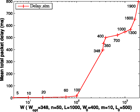
Total packet delay in ms when W varies and W opt=348 for a two-AC EDCA network without a backoff mechanism. Note that W<W opt corresponds to k>k opt
-
When W<348, the total delay is low. Particularly, when W is far less than 348, the total delay is much low. For example, when W decreases from 100 to 5, the total delay decreases from tens of milliseconds to several milliseconds. The main reason is, as explained in Fig. 2, over this interval, the system traffic load is very light and is far less than the saturated load; therefore, each arrived packet can be delivered to the receiver quickly, leading to a much low delay.

Figures 4 and 5, respectively, repeats Figs. 2 and 3, except that only the HP AC exists (i.e., it is the DCF system without a backoff mechanism), n=30, L=500 bytes, k opt=0.1904, and W opt=315. As expected, the results observed in the DCF system are very similar to those in the two-AC system, when k s ≤k opt and k s >k opt.

Maximum stable HP throughput when W varies and W opt=315 for a DCF network without a backoff mechanism. Note that W<W opt corresponds to k>k opt

Total packet delay in milliseconds when W varies and W opt=315 for a DCF network without a backoff mechanism. Note that W<W opt corresponds to k>k opt
Experiment 3 to illustrate the performance similarity when Wmin ≠ Wmax and when Wmin = Wmax: To illustrate that a DCF system with Wmin ≠Wmax exhibits throughput and delay properties that are very similar to that with Wmin =Wmax, we consider the default EDCA CW configuration for voice traffic, namely, [Wmin, Wmax] = y[8, 16]. We map the CW configuration with Wmin ≠Wmax to that with Wmin =Wmax \(\triangleq \left [2/\beta _{s}-1\right ] \), where β s is the saturated attempt rate for Wmin ≠Wmax. For example, when n=30, L=500 bytes, we have the CW mapping: [Wmin, Wmax] = [8, 16] → [Wmin, Wmax] = [13, 13] and k s =n β s =30×2/(13+1)=4.2857≫k opt=0.1904. We then consider Poisson traffic and run simulations to obtain the following simulation results. Table 2 compares the maximum stable throughput, the saturated throughput, and the total delay before and after mapping and shows that the mapping pair has very similar performance. From this table, when Wmin ≠Wmax, the corresponding simulation results are respectively 1.9731 and 0.2038 Mbps, 1.7398 ms; when Wmin =Wmax, they are respectively 1.9751 Mbps, 0.2042 Mbps, and 1.9743 ms. This comparison indicates that like Wmin =Wmax, when k s is sufficiently greater than k opt, the DCF system when Wmin ≠Wmax may achieve a stable throughput far higher than the saturated throughput, while providing satisfactory QoS.
Experiment 4 to verify the effectiveness of the proposed idle-sense-based scheme: The fourth experiment considers CBR voice traffic and determines the maximum number of admitted HP nodes, n max, that ensures throughput stability, when the idle-sense-based scheme is used, and for the static cases of W=300 and 20. We take the theoretical value of n max to be ⌊Γ(k opt)/(λ L)⌋ for the adjustable HP CW case and ⌊Γ(k s )/(λ L)⌋ for the static HP CW case. The simulation value of n max is the maximum number of HP nodes satisfying (8). In this experiment, we calculate n max when all HP nodes are assigned, alternately, the G.711-100, G.711-50, iLBC, G.729, and G.723a voice codecs (which are shown in Table 3 and are from Table IV (b) in [31]), where each type of voice traffic is modeled as CBR traffic. The theoretical and simulation values of n max are listed in Table 4. We now explain the obtained results.
-
In the case of the idle-sense-based scheme, Table 4 shows that each simulation value of n max is exactly equal to its theoretical value (except for the G.711-50 voice codec) and is the maximum (except for the G.723a voice codec) when compared with the cases of W=300 or W=20. At the same time, we also observe that the total delay for each voice codec is less than 25 ms. This manifests that (i) the idle-sense-based scheme can maximize the stable HP throughput while maintaining a low total delay and (ii) Γ(k opt) is a tight upper bound on the stable throughput for the idle-sense-based scheme.
Table 3 Parameters for voice packets Table 4 Comparison of n max between the theoretical results and the simulation results for voice codecs shown in Table 3 -
For the case of W=300, we have W≥W opt. From Table 4, the prediction error of n max between the theoretical and simulation results for each voice codec is at most one. This indicates that Γ(k s ) is a tight upper bound on the stable throughput, as expected in this case. However, the total delay for each voice codec except G.711-50 is significantly larger than 25 ms.
-
For the case of W=20, we have W<W opt. From Table 4, the prediction of n max is reasonably accurate for the G.711-100 and G.711-50 voice codecs since W=20 approximates their respective optimal CWs, but the prediction is far less accurate for the iLBC, G.729, and G.723a voice codecs since W=20 is far less than their respective optimal CWs. This indicates that the saturation throughput might significantly underestimate the maximum stable throughput, as expected in this case. Comparing the case of W=300 with the cases of W=20, we can see that each simulation value of n max in the latter is reasonably less than that in the former. However, the total delay for each voice codec is less than 25 ms in the latter and hence is significantly less than that in the former. This indicates that it is attractive to set a small CW value in order to obtain a satisfactory quality of service.
5 Conclusions
In wireless cyber-physical systems, more and more data will be transmitted over wireless networks such as 802.11 networks. To fully utilize the bandwidth of 802.11 networks for supporting wireless CPS applications, in this paper, we study the maximum stable throughput in 802.11 networks. We reveal that the maximum stable throughput follows different rules in two partitioned intervals and point out that failing to differentiate the two intervals is the fundamental reasons causing the existing contradictory conclusions. Applying the rules, we assert that for the parameter settings in 802.11 EDCA standard, high-priority traffic can achieve a stable throughput far higher than the saturation throughput, which contradicts the existing augments. Furthermore, we propose a CW-adjustable scheme to maximize the stable throughput of high-priority traffic. This study provides new insights on the unsaturation performance and helps utilize the limited bandwidth of wireless networks fully.
6 Appendix
Proof of Theorem ??.
We first prove that 0<η<1. Note that
If \(T_{b}\geq T_{b_{0}}\phantom {\dot {i}\!}\), we have
On one hand, since \(T_{b}\geq T_{b_{0}}\phantom {\dot {i}\!}\) and \(\phantom {\dot {i}\!}T_{b_{0}}\gg \sigma \), we have
On the other hand, since 0<C 0<1, we have
In short, when \(T_{b}\geq T_{b_{0}}\phantom {\dot {i}\!}\), we have 0<η<1.
If \(\phantom {\dot {i}\!}T_{b}<T_{b_{0}}\), we have
On one hand, since T b ≫σ and 0<C 0<1, we have
On the other hand, since 0<T b −σ<T b , we have
In short, when \(T_{b}<T_{b_{0}}\phantom {\dot {i}\!}\), we have 0<η<1.
We now prove (a). First, we note
Then, applying the Poisson distribution to approximate the binomial distributions in (1) and (2), we have
and
Next, we calculate Γ(k) as follows.
We now prove (b). To maximize Γ(k), we set the first derivative of Γ(k) to zero and have
Hence, we have
Finally, since only \(\mathcal {W}_{0}(-\eta e^{-1})>-1\) for −η e −1∈(−1/e,0), we have
\(\blacksquare \)
References
EA Lee, Cyber physical systems: design challenges, Technical Report No. UCB/EECS-2008-8. Available at http://www.eecs.berkeley.edu/Pubs/TechRpts/2008/EECS-2008-8.pdf.
W Kang, K Kapitanova, SH Son, RDDS: a real-time data distribution service for cyber-physical systems. IEEE Trans. Ind. Inform.8(2), 393–405 (2012).
EA Lee, The past, present and future of cyber-physical systems: a focus on models. Sensors. 15:, 4837–4869 (2015).
S Cheng, Z Cai, J Li, X Fang, in INFOCOM. Drawing dominant dataset from big sensory data in wireless sensor networks (IEEE, 2015). http://ieeexplore.ieee.org/xpl/login.jsp?tp=&arnumber=7218420&url=http%3A%2F%2Fieeexplore.ieee.org%2Fxpls%2Fabs_all.jsp%3Farnumber%3D7218420.
J Li, S Cheng, H Gao, Z Cai, Approximate physical world reconstruction algorithms in sensor networks. IEEE Trans. Parallel Distrib. Syst.25(12), 3099–3110 (2014).
S Cheng, Z Cai, J Li, Curve query processing in wireless sensor networks. IEEE Trans. Veh. Technol.64(11), 5198–5209 (2015).
BJ Kwak, NO Song, LE Miller, Performance analysis of exponential backoff. IEEE/ACM Trans. Networking. 13(2), 343–355 (2005).
H Zhai, X Chen, Y Fang, How well can the IEEE 802.11 wireless LAN support quality of service?IEEE Trans. Wirel. Commun.4(6), 3084–3094 (2005).
X Zheng, J Li, H Gao, Z Cai, Capacity of wireless networks with multiple types of multicast sessions. MOBIHOC (ACM New York, NY, USA, 2014). http://dl.acm.org/citation.cfm?id=2632985.
Z Cai, Z Chen, G Lin, A 3.4713-approximation algorithm for the capacitated multicast tree routing problem. Theor. Comput. Sci.410(52), 5415–5424 (2008).
Z Cai, R Goebel, G Lin, Size-constrained tree partitioning: approximating the multicast k-tree routing problem. Theor. Comput. Sci.412(3), 240–245 (2011).
Z Cai, G Lin, G Xue, in Proceedings of 11th Annual International Conference on Computing and Combinatorics 2005(COCOON). Improved approximation algorithms for the capacitated multicast routing problem (Springer Berlin Heidelberg, 2005), pp. 136–145. http://link.springer.com/chapter/10.1007%2F11533719_16.
X Guan, A Li, Z Cai, T Ohtsuki, Continuous data aggregation and capacity in probabilistic wireless sensor networks. Mob. Netw. Appl.20(2), 147–156 (2015).
N Abramson, The ALOHA system—another alternative for computer communication. Proc. Fall Joint Comput. Conf. AFIP Conference. 44:, 281–285 (1970).
IEEE Std. 802.11-2007, Part 11: Wireless LAN Medium Access Control (MAC) and Physical Layer (PHY) Specifications, June 2007.
L Dai, Stability and delay analysis of buffered ALOHA networks. IEEE Trans. Wirel. Commun.11(8), 2707–2719 (2012).
G Fayolle, E Gelenbe, J Labetoulle, Stability and optimal control of the packet switching broadcast channel. J. Assoc. Comput. Mach.24(3), 375–386 (1977).
WA Rosenkrantz, D Towsley, On the instability of the slotted ALOHA multiaccess algorithm. IEEE Trans. Automat. Contr.28(10), 994–996 (1983).
YJ Zhang, SC Liew, DR Chen, Sustainable throughput of wireless LANs with multipacket reception capability under bounded delay-moment requirements. IEEE Trans. Mob. Comput.9(9), 1226–1241 (2010).
L Dai, X Sun, A unified analysis of IEEE 802.11 DCF networks: Stability, throughput and delay. IEEE Trans. Mob. Comput.12(8), 1558–1572 (2013).
H Zhai, Y Kwon, Y Fang, Performance analysis of IEEE 802.11 MAC protocols in wireless LANs. Wirel. Commun. Mob. Comput.4(8), 917–931 (2004).
D Malone, K Duffy, D Leith, Modeling the 802.11 distributed coordination function in non-saturated heterogeneous conditions. IEEE/ACM Trans. Networking. 15(1), 159–172 (2007).
X Yao, W Wang, S Yang, Y Cen, X Yao, T Pan, IPB-frame adaptive mapping mechanism for video transmission over IEEE 802.11e WLANs. Comput. Commun. Rev.44(2), 5–12 (2014).
Y Javed, A Baig, M Maqbool, Enhanced quality of service support for triple play services in IEEE 802.11 WLANs. EURASIP J. Wirel. Commun. Netw.2015(1), 1–14 (2015).
F Cali, M Conti, E Gregori, Dynamic tuning of the IEEE 802.11 protocol to achieve a theoretical throughput limit. IEEE/ACM Trans. Networking. 8(6), 785–799 (2000).
M Heusse, F Rousseau, R Guillier, A Duda, in Proceedings of ACM Sigcomm. Idle sense: an optimal access method for high throughput and fairness in rate diverse wireless LANs (ACM New YorkNY, USA, 2005). http://dl.acm.org/citation.cfm?id=1080107.
G Bianchi, Performance analysis of the IEEE 802.11 distributed coordination function. IEEE J. Sel. Areas Commun.18(3), 535–547 (2000).
QL Zhao, DHK Tsang, T Sakurai, Modeling nonsaturated IEEE 802.11 DCF networks under arbitrary buffer size. IEEE Trans. Mob. Comput.10(9), 1248–1263 (2011).
RM Corlessa, GH Gonnet, DEG Hare, DJ Jeffrey, DE Knuth, On the Lambert W function. Adv. Comput. Math.5:, 329–359 (1996).
D Chiu, R Jain, Analysis of the increase and decrease algorithms for congestion avoidance in computer networks. J. Comput. Networks ISDN. 17(1), 1–14 (1989).
QL Zhao, DHK Tsang, T Sakurai, A simple critical-offered-load-based CAC scheme for IEEE 802.11 DCF networks. IEEE/ACM IEEE/ACM Trans. Networking. 19(5), 1485–1498 (2011).
Acknowledgements
This work is partially supported by the Macao Science and Technology Development Fund under Grant (No. 104/2014/A3 and No. 013/2014/A1), NNSF of China under Grant 61373027 and NSF of Shandong Province under Grant ZR2012FM023.
Author information
Authors and Affiliations
Corresponding author
Additional information
Competing interests
The authors declare that they have no competing interests.
Rights and permissions
Open Access This article is distributed under the terms of the Creative Commons Attribution 4.0 International License(http://creativecommons.org/licenses/by/4.0/), which permits unrestricted use, distribution, and reproduction in any medium, provided you give appropriate credit to the original author(s) and the source, provide a link to the Creative Commons license, and indicate if changes were made.
About this article

Cite this article
Zhao, Q., Sakurai, T., Yu, J. et al. Maximizing the stable throughput of high-priority traffic for wireless cyber-physical systems. J Wireless Com Network 2016, 53 (2016). https://doi.org/10.1186/s13638-016-0551-2
Received:
Accepted:
Published:
DOI: https://doi.org/10.1186/s13638-016-0551-2