A frequency-sharing weather radar network system using pulse compression and sidelobe suppression

Abstract

To mitigate damages due to natural disasters and abruptly changing weather, the importance of a weather radar network system (WRNS) is growing. Because radars in the current form of a WRNS operate in distinct frequency bands, operating a WRNS consisting of a large number of radars is very costly in terms of frequency resource. In this paper, we propose a novel WRNS in which multi-site weather radars share the same frequency band. By employing pulse compression with nearly orthogonal polyphase codes and sidelobe removal processing, a weather radar of the proposed frequency-sharing WRNS addresses inter-site and intra-site interferences simultaneously. Through computer simulations, we show the feasibility of the proposed system taking the performance requirement of a typical single weather radar into account.

1 Introduction

The number of natural disasters has been increasing sharply since 1970 [1]. According to the statistics report in [2], over 330 natural disasters occurred in 2013 and took lives of a significant number of people (21,610) and caused serious economic damages ($156.7 billion). In an attempt to prevent damages from natural disasters, several research institutes (e.g., Oklahoma University) and governmental agencies (e.g., National Oceanic and Atmosphere Administration (NOAA)) have been collaborating with each other to develop a weather radar network system (WRNS) that enables forecasting unusual weather phenomena effectively.

A WRNS is composed of multiple weather radars, which are deployed in different geographical positions for monitoring the weather phenomena nearby. More specifically, each radar transmits radio pulse signal periodically, captures the signal that has been backscattered from weather targets, and extracts important parameters from the signal (e.g., reflectivity and radial velocity) for characterizing the current weather status. Although the current form of a WRNS works adequately, it has a significant limitation in terms of the frequency efficiency.

Frequency spectrum is a fundamental resource for wireless communication and remote sensing, but we lack the resource due to explosive demands for mobile communications. Despite the problem of frequency scarcity, the goal of the current deployment of a WRNS is not aligned with the frequency efficiency. To be specific, radars in the current WRNSs operate in distinct frequency bands; thus, the total bandwidth that is required for a WRNS increases linearly with the number of radar deployments. For example, in the US WRNS, 160 radars are deployed throughout the USA, each of which requires 5 MHz bandwidth [3]. Although a frequency reuse scheme can be employed in the deployment, we must allocate a significantly wide frequency band to the WRNS, which is extremely costly.

A simple solution is to make multiple radars share the same frequency band. Frequency sharing can be realized by operating radars separately in other domains than the frequency domain: as in wireless communications area, we can consider the time domain and code domain. In the approach of frequency sharing by separating radars in the time domain, only one radar operates for a certain period of time and, after the period, one of the other radars starts to operate in a given order. The main problem in this approach is that the time interval from a radar’s pulse emission to the next pulse emission grows linearly with the number of radars that share the spectrum. Due to the limitation of observation time, the increase in the pulse-to-pulse time interval reduces the amount of sensing data averaged over the whole observation time, which degrades estimation and forecasting accuracies.

In this paper, we consider frequency sharing by separating radars in the code domain, in which each radar is distinguished by exploiting its own code “orthogonal” to those of the other radars. (In a WRNS, the word “orthogonal” is used in a different sense, which will be defined in Section 3). By separating the radars of a WRNS in the code domain, we can avoid the problem of the decrease in estimation accuracy in the time domain approach. In the code domain approach, we need to employ the technique of pulse compression [4]. Pulse compression is a technique employed in a single radar (which is not necessarily a weather radar) system in order to improve the performances of range resolution and sensitivity together under the limited peak power. Meanwhile, in this paper, the technique of pulse compression is adopted for achieving the objective of frequency sharing in a WRNS in combination with orthogonal codes. Specifically, a radar transmits a pulse modulated with its own (pulse compression) code in waveform generation; on the reception mode, the radar can extract its own signal by canceling out the signals from other radars via the matched filter (MF).

Translating the idea of frequency sharing by using orthogonal codes into a feasible WRNS is an extremely difficult problem in itself. The difficulty is mainly attributed to the extremely significant signal interferences, which hinder accurate estimation of weather parameters. The interferences in a WRNS can be categorized into (1) inter-site interference and (2) intra-site interference.

Inter-site interference occurs when multiple radars share the same frequency band. Specifically, a signal associated with one radar can interfere with those associated with other radars. The interference inevitably distorts the received signals of the radars, thereby leading to inaccurate estimations of weather parameters. On the other hand, intra-site interference happens even when there is only one radar operating in the frequency band. It can be regarded as a kind of self-interference due to partial overlap of the multiple backscattered signals that occur when the radar signal is backscattered by closely located multiple targets. This intra-site interference becomes highly serious in a radar system that employs a long pulse (e.g., pulse compression radar) and that deals with volume-type targets (e.g., weather radar).

There have been several studies to mitigate inter-site interferences by proposing nearly orthogonal codes. In [5], an algorithm was proposed for deriving nearly orthogonal codes that can be exploited in multi-static radar network systems. In [6, 7], a design framework was proposed for generating polyphase codes that can be adopted for orthogonal netted radar systems. On the other hand, several studies have focused on mitigating intra-site interferences. For example, in [8], an algorithm was proposed to use an inverse filter in order to reconstruct real peaks from the received signal. In [9], effective sidelobe suppression algorithms were introduced for discrete point targets and contiguous scattering targets, which we refer to as the CLEAN algorithm in this paper. In [10], a combination of the phase distortion and spectrum modification techniques was proposed for sidelobe suppression in a single weather radar with pulse compression. Unfortunately, none of the previous approaches in [5–10] is appropriate to successfully address the two challenges (intra-site and inter-site interferences) simultaneously.

In this paper, we propose a novel WRNS in which multi-site weather radars operate in the same frequency band, with the key issue of overcoming the two challenges described above simultaneously. The proposed system suppresses the inter-site interference by adopting pulse compression with nearly orthogonal codes, and at the same time, removes the intra-site interference based on a well-known sidelobe suppression mechanism. Through computer simulations, the proposed frequency-sharing WRNS is shown to be feasible even when the performance requirement of conventional single weather radar systems is applied.

The following two points set our work apart from previous works on weather radar systems:

• The novelty of this paper mainly lies in the design of an architecture of a novel WRNS that enables the constituent radars to share the same frequency band. In Fig. 1, we have presented the architecture of the proposed frequency-sharing WRNS. In the transmission mode, each radar transmits a pulse modulated with a distinct code from nearly orthogonal pulse compression codes. Then, in the reception mode, each radar captures signals backscattered by weather targets, which contain the signals originated from other radars also. The received signal first goes through the MF, which results in suppression of the inter-site interference. Subsequently, by applying an additional process of sidelobe suppression, the intra-site interference is mitigated effectively.

  Fig. 1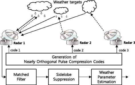

  

  System architecture of the proposed frequency-sharing WRNS

• We have conducted an elaborate study on feasibility of the WRNS. Specifically, the estimation accuracies on two weather parameters, reflectivity and velocity, satisfied the performance requirements of a typical single weather radar, WSR-88D, under the expected SIR condition. To the best of our knowledge, this study is the first to validate the feasibility of frequency-sharing weather radar systems.

The rest of this paper is organized as follows. We will first present the system model of a WRNS in Section 2. In Section 3, the key techniques for frequency sharing in the WRNS are described. Next, the performance of the proposed system is evaluated through computer simulations in Section 4. Finally, our work will be concluded in Section 5.

2 System model

In this section, we present a system model of a WRNS, which is defined as a group of weather radars that have the same prior information (e.g., code set) and reside in the same frequency channel. Before explaining the details, we have first summarized the nomenclature and main assumptions of this paper in Tables 1 and 2. The assumption on reflection model is made because granularity for measuring weather parameters is a range bin in reality. By using a virtual point target for representing weather scatterers (hydrometeors) in each range bin, we can greatly simplify the reflection model while maintaining estimation accuracies on weather parameters. For this reason, this assumption has been used in a number of weather radar studies [8, 11]. The second assumption is made because this feasibility study focuses on weather conditions in which a target velocity rarely changes over the observation time as in the case of, for example, (stable) rain fall or snow fall.

Table 1 Nomenclature

Table 2 Main assumptions

Assume a WRNS consisting of N mono-static weather radars with pulse compression, where the nth radar is denoted by Radar-n. To understand how each radar can extract weather parameters in the presence of other radar signals, we focus on the operations of removing interferences and reconstructing target information in a specific radar (we call this radar the main radar) and regard the other radars as interferers (we call these radars interfering radars). Without loss of generality, we consider Radar-1 as the main radar and Radars- 2,3,⋯,N as interfering radars throughout this paper.

Each radar periodically switches its antenna mode between the transmission and reception modes. Specifically, in the transmission mode, the radar transmits its pulse in the current direction of the antenna; it switches the mode to the reception mode and captures radar signals in the air for a while. Then, it switches back to the transmission mode for transmitting the next pulse. Here, the interval between two adjacent transmissions is called the pulse repetition time (PRT), and is denoted by T. Note that, in order to improve observation performance for a specific direction, a radar stays in the direction during a number of repetitions of the two modes: we denote this number of repetitions by K.

2.1 Pulse transmission

We assume that all the radars in the WRNS considered in this study employ pulse compression. The purpose of employing pulse compression in our system is entirely different from that in conventional single radar systems. In conventional single radars, pulse compression is employed in order to improve both performances of range resolution and sensitivity (i.e., target detection capability) under the limitation of peak power [12]. On the other hand, in the WRNS of this study, pulse compression is for removing interferences from other radars by employing mutually uncorrelated codes, which will be addressed in detail in Section 3.

In the transmission mode, Radar-1 transmits a pulse modulated with its own code, where each sub-pulse represents an element of the code in order. Let us denote the pulse (equivalently, pulse compression code) of Radar-1 by

$$\begin{array}{@{}rcl@{}} \boldsymbol s_{1} = \left[ s_{1}[\!1], s_{1}[\!2], \cdots, s_{1}[\!L]\!\right], \end{array} $$

((1))

where L is the code length and corresponds to the pulse duration time τ=L Δ τ. Here, Δ τ denotes the sub-pulse duration time.

2.2 Reflection of pulse by weather targets

As illustrated in Fig. 2, a pulse transmitted by Radar-1 is reflected by weather targets and returns to Radar-1. Whenever the pulse is reflected by a weather target, its amplitude and phase change according to the reflectivity and velocity of the target. As a weather target actually consists of a tremendous number of weather scatterers, it is extremely difficult to individually consider and model the impact of each scatterer on the reflection of the radar signal. Thus, we employ a simple approach that has been adopted and validated in many previous studies [8, 11]. In the approach, the radar signal’s path is divided into multiple resolution volumes (a.k.a. range bins) and it is assumed that there exists a single virtual point target in each range bin. Then, the channel impulse response of a target is defined as the aggregated impacts of all scatterers in the corresponding range bin on the reflection. This approach is illustrated in Fig. 2, in which a series of black circles indicates the virtual (point) targets. For further simplification, we integrate the effect of signal propagation into the channel responses of the targets.

Fig. 2

System model of a WRNS

Let

$$\begin{array}{@{}rcl@{}} \boldsymbol h_{1}^{(k)} = \left[h_{1}^{(k)}[\!1], h_{1}^{(k)}[\!2], \cdots, h_{1}^{(k)}[\!L_{T}] \right] \end{array} $$

((2))

denote the impulse response of the reflection channel for the kth (k=1,2,⋯,K) transmitted pulse of Radar-1, which returns the pulse to its source. Here, L _T =T/Δ τ is the length equivalent to the PRT. As described above, the reflection channel represents all the reflections caused by the virtual weather targets in the direction that the antenna of Radar-1 is facing. Specifically, the impulse response $h_{1}^{(k)}[\!i]$ of the ith virtual target can be expressed as

$$\begin{array}{@{}rcl@{}} h_{1}^{(k)}[\!i]=A_{1}[\!i]\text{exp}\left\{j\phi_{1}^{(k)}[\!i]\right\}. \end{array} $$

((3))

The amplitude A ₁[ i]>0 in (3) is dependent on the reflectivity of the weather target as

$$\begin{array}{@{}rcl@{}} {A_{1}^{2}}[i] = k_{R} \frac{G_{t}G_{r} Z_{1}[\!i]}{{d_{1}^{2}}[\!i]} \end{array} $$

((4))

based on the weather radar equation [13]. Here, Z ₁[ i] is the reflectivity of the ith target in the current direction of Radar-1, $d_{1}[\!i] = \frac {1}{2}ci \Delta \tau$ is the distance between the target and radar with c denoting the speed of light, G _t and G _r are the antenna gains for transmission and reception, respectively, and the constant k _R depends on the radar parameters such as 3-dB beamwidth, pulse duration time, and wavelength. Note that G _t and G _r rely on the path of the radar signal, which will be addressed in detail later in Section 4.1.3.

The phase $\phi _{1}^{(k)}[\!i]$ in (3) is associated with the velocity of the weather target. Specifically, it can be expressed as [14]

$$\begin{array}{@{}rcl@{}} \phi_{1}^{(k)}[\!i] = k \varphi_{1}[\!i] + \Delta \varphi_{1} [\!i], \end{array} $$

((5))

where

$$\begin{array}{@{}rcl@{}} \varphi_{1}[\!i] = -\frac{4\pi T}{\lambda} v_{1}[\!i] \end{array} $$

((6))

is the average phase change for the PRT due to the (average) radial velocity v ₁[ i] of the ith target and λ is the wavelength of the radar signal. The term Δ φ ₁[ i] indicates the variance of the phase change, which is associated with the variation of the velocity of the target. In this feasibility study, we assume Δ φ ₁[ i]=0 for simplicity.

2.3 Reception of reflected pulses

If we ignore the signals of interfering radars, we can express the signal received in the kth reception mode of Radar-1 by $\boldsymbol s_{1} * \boldsymbol h_{1}^{(k)} + \boldsymbol n$. Here, n is a complex Gaussian noise with mean zero. Now recall that there exist other weather radars (Radars-2, 3, ⋯, N), the signals of which could interfere with that of Radar-1. Taking this into account, we have the received signal as

$$\begin{array}{@{}rcl@{}} \boldsymbol r^{(k)} = \boldsymbol s_{1} * \boldsymbol h_{1}^{(k)} + \sum\limits_{n=2}^{N} \boldsymbol s_{n} * \boldsymbol g_{n,1} +\boldsymbol n. \end{array} $$

((7))

Here, for n=2,3,⋯,N, g _n,1 is the impulse response of the reflection channel between the interfering Radar-n and the main Radar-1.

In (7), the term $\boldsymbol s_{1} * \boldsymbol h_{1}^{(k)}$ contains the intra-site interference mentioned in Section 1: specifically, the difference between $\boldsymbol s_{1} * \boldsymbol h_{1}^{(k)}$ and $\boldsymbol h_{1}^{(k)}$ can be considered as the intra-site interference. On the other hand, the term $\sum \limits _{n=2}^{N} \boldsymbol s_{n} * \boldsymbol g_{n,1}$ corresponds to the inter-site interference.

2.4 Problem definition

To introduce a WRNS that shares the same frequency band, the main challenge lies in overcoming signal distortion that results from the intra-site and inter-site interferences. Such distortion hinders accurate estimation of weather parameters such as the reflectivity and velocity. We can formulate this problem as follows:

Problem: Given the received signals $\left \{\boldsymbol r^{(k)}\right \}_{k=1}^{K}$ at Radar-1, which have been contaminated by both of the intra-site and inter-site interferences, estimate the reflectivity Z ₁ and velocity v ₁ of the weather targets.

Our problem is, roughly speaking, to estimate the reflection channel $\boldsymbol h_{1}^{(k)}$, sometimes called the main reflection channel, because the reflectivity and velocity are directly related with the amplitude and phase of $\boldsymbol h_{1}^{(k)}$ as shown in (3)–(6).

3 Key techniques for frequency sharing

In order to solve the problem of this study, we employ two key techniques: (1) pulse compression with a nearly orthogonal code set and (2) signal processing for sidelobe suppression that further refines the output of the MF.

Let us now describe the details.

3.1 Pulse compression with (nearly) orthogonal code set

3.1.1 Matched filtering

The received signal (7) in Radar-1 is fed into the MF that matches the transmitted pulse, the output of which is given as

$$\begin{array}{@{}rcl@{}} \boldsymbol y_{MF}^{(k)} &=& \boldsymbol r^{(k)} * \boldsymbol s_{1}^{MF} \\ &=& \boldsymbol h_{1}^{(k)}*\boldsymbol R_{1,1} + \sum\limits_{n=2}^{N} \boldsymbol g_{n,1}*\boldsymbol R_{n,1} +\boldsymbol n * \boldsymbol s_{1}^{MF}, \end{array} $$

((8))

where

$$\begin{array}{@{}rcl@{}} \boldsymbol s_{1}^{MF} = \frac{1}{L} \times \left[ s_{1}[\!L], s_{1}[\!L-1], \cdots, s_{1}[\!1] \right] \end{array} $$

((9))

is the impulse response of the MF of Radar-1. Here, $\boldsymbol R_{n_{1},n_{2}}\,=\,\left [ R_{n_{1},n_{2}}[\!-L\,+\,1], R_{n_{1},n_{2}}[\!-L\,+\,2], \cdots, R_{n_{1},n_{2}}[\!L\,-\,1]\!\right ]$ is the normalized correlation of $\boldsymbol s_{n_{1}}$ and $\boldsymbol s_{n_{2}}$ defined by

$$\begin{array}{@{}rcl@{}} R_{n_{1},n_{2}}[\!i] = \frac{1}{L} \sum\limits_{j=\max(1,1-i)}^{\min(L,L-i)} s_{n_{1}}[\!j]s_{n_{2}}^{*}[\!j+i] \end{array} $$

((10))

for i=−L+1,−L+2,⋯,L−1 and n ₁,n ₂=1,2,⋯,N: it is the autocorrelation if n ₁=n ₂; otherwise, it is the cross-correlation.

3.1.2 Orthogonal code set

Let us denote the set of pulse compression codes by the N×L matrix

$$\begin{array}{@{}rcl@{}} S = \left[\begin{array}{cccc} s_{1}[\!1] & s_{1}[\!2] & \cdots & s_{1}[\!L] \\ \vdots & \ddots & \vdots \\ s_{N}[\!1] & s_{N}[\!2] & \cdots & s_{N}[\!L] \end{array}\right], \end{array} $$

((11))

where the nth row corresponds to s _n . Now assume that S satisfies

$$\begin{array}{@{}rcl@{}} R_{n,n}[i] = \left\{\begin{array}{ll} 1, & \ i=0\\ 0, & \ i\neq0\end{array}\right. \end{array} $$

((12))

for n=1,2,⋯,N, and

$$\begin{array}{@{}rcl@{}} R_{n_{1},n_{2}}[\!i] = 0, \ \ \ \ \text{all~}i \end{array} $$

((13))

for n ₁≠n ₂. In this paper, we will refer to such a code set as an orthogonal code set.

When an orthogonal code set is employed, the output of the MF in (8) is simply given as

$$\begin{array}{@{}rcl@{}} \boldsymbol y_{MF}^{(k)} = \boldsymbol h_{1}^{(k)} + \boldsymbol n * \boldsymbol s_{1}^{MF}. \end{array} $$

((14))

Here, as the magnitude of the noise n is normally very small compared with $\left |\boldsymbol h_{1}^{(k)}\right |$, $\boldsymbol y_{MF}^{(k)}$ can be considered as an approximated $\boldsymbol h_{1}^{(k)}$. In addition, because

$$\begin{array}{@{}rcl@{}} Z_{1} [i] &=& \frac{{d_{1}^{2}}[\!i]}{k_{R} G_{t} G_{r}} {A_{1}^{2}} [\!i] \\ &=& \frac{{d_{1}^{2}}[\!i]}{k_{R} G_{t} G_{r}} \left| h_{1}^{(k)} [\!i]\right|^{2}, \ \text{for any~} k \in \left\{1,2,\cdots,K\right\} \\ &=& \frac{{d_{1}^{2}}[\!i]}{k_{R} G_{t} G_{r}} \frac{1}{K} \sum\limits_{k=1}^{K} \left| h_{1}^{(k)} [\!i]\right|^{2} \end{array} $$

((15))

from (3) and (4), the estimate $\hat {Z}_{1}[\!i]$ of the reflectivity Z ₁[ i] can be obtained as

$$\begin{array}{@{}rcl@{}} \hat{Z}_{1} [\!i] &=& \frac{{d_{1}^{2}}[\!i]}{k_{R} G_{t} G_{r}} \frac{1}{K} \sum\limits_{k=1}^{K} \left| y_{MF}^{(k)}[\!i] \right|^{2}. \end{array} $$

((16))

Here, the replacement of “for any k” with the average over k is for reducing the estimation error due to the noise. Similarly, because

$$ \begin{aligned} v_{1} [\!i] &= -\frac{\lambda}{4 \pi T} \left({\phi}_{1}^{(k+1)}[\!i] - \phi_{1}^{(k)}[\!i] \right), \text{for any} \ k \in \left\{1,2,\cdots,K-1\right\} \\ &= -\frac{\lambda}{4 \pi T} \angle{\left\{ h_{1}^{(k+1)}[\!i] \left(h_{1}^{(k)}[\!i]\right)^{*} \right\}}, \ \text{for any~} k \in \left\{1,2,\cdots,K-1\right\} \\ &= - \frac{\lambda}{4 \pi \!T} \frac{1}{K-1}\sum\limits_{k=1}^{K-1} \angle{\left\{ h_{1}^{(k+1)}[\!i] \left(h_{1}^{(k)}[\!i]\right)^{*} \right\}} \end{aligned} $$

((17))

from (3), (5), and (6), the estimate $\hat {v}_{1}[\!i]$ of the reflectivity v ₁[ i] can be obtained as

$$\begin{array}{@{}rcl@{}} \hat{v}_{1} [\!i] = - \frac{\lambda}{4 \pi T} \frac{1}{K-1}\sum\limits_{k=1}^{K-1} \angle{\left\{ y_{MF}^{(k+1)}[\!i] \left(y_{MF}^{(k)}[\!i]\right)^{*} \right\}}. \end{array} $$

((18))

3.1.3 Design of nearly orthogonal code set

It is impossible to design an orthogonal code set that perfectly satisfies both (12) and (13). Hence, an alternative is to design a code set that satisfies the conditions as closely as possible. In this paper, we call such a code set a nearly orthogonal code set.

There have been many studies on designing nearly orthogonal code sets [5–7, 15]. For example, in the design method proposed in [5], a simple full search algorithm was employed based on Hadamard and Fourier matrices that have the property $R_{n_{1},n_{2}}[\!0] = 0$ for n ₁≠n ₂: it is noteworthy that the cost function of this method is defined in terms of the peak values of correlations, not energies. In [6], a hybrid optimization method combining simulated annealing (SA) with a traditional iterative code selection was proposed to design a nearly orthogonal polyphase code set. In [7], another optimization method based on cross entropy technique was proposed, where a structural constraint to maintain Doppler tolerance was considered together with the orthogonality conditions.

Among the previously proposed methods for designing nearly orthogonal code sets, we adopt the polyphase code design method in [6]. The cost function of the design method is given by

$$ E = \sum\limits_{n=1}^{N} \sum\limits_{i=1}^{L-1} \left|R_{n,n}[\!i]\!\right|^{2}\,+\, \alpha \sum\limits_{n_{1}=1}^{N-1}\sum\limits_{n_{2}=n_{1}+1}^{N}\sum\limits_{i=-L+1}^{L-1}\left|R_{n_{1},n_{2}}[\!i]\!\right|^{2}, $$

((19))

where the first term is the sum of sidelobe energies of autocorrelations and the second term is the sum of cross-correlation energies. Here, α≥0 is the weighting coefficient. The minimization of (19) is accomplished through two steps: the first step is to reach near the global minimum by employing SA, and the second is to tune the solution more finely by an iterative code selection algorithm. The detailed procedure of the design method can be summarized as in Table 3.

Table 3 Procedure for the design of a nearly orthogonal polyphase code set

Once we design a nearly orthogonal code set, the performance of the designed code set can be quantified by the following two measures: the autocorrelation sidelobe peak (ASP)

$$\begin{array}{@{}rcl@{}} ASP(n) = 20 \log \left(\max\limits_{i \neq 0} \left|R_{n,n}[\!i]\right| \right) \end{array} $$

((20))

of the nth code, and cross-correlation peak (CP)

$$\begin{array}{@{}rcl@{}} CP(n_{1},n_{2}) = 20 \log \left(\max \left|R_{n_{1},n_{2}}[\!i] \right|\right) \end{array} $$

((21))

of the n ₁th and n ₂th codes (n ₁≠n ₂) in dB. Considering conditions (12) and (13) of an orthogonal code set, it is clear that the smaller the values of ASPs and CPs of a nearly orthogonal code set are, the closer the code set is to an orthogonal code set.

3.2 Iterative sidelobe removal

When a nearly orthogonal code set is employed for pulse compression, the output of the MF in (8) can be rewritten as

$$ \boldsymbol y_{MF}^{(k)} = \boldsymbol h_{1}^{(k)} + \boldsymbol h_{1}^{(k)}* \bar{\boldsymbol R}_{1,1} + \sum\limits_{n=2}^{N} \boldsymbol g_{n,1}*\boldsymbol R_{n,1} +\boldsymbol n * \boldsymbol s_{1}^{MF}, $$

((22))

where $\bar {\boldsymbol R}_{1,1}$ is the sidelobe component of R ₁ with the ith element

$$\begin{array}{@{}rcl@{}} \bar{R}_{1,1} [\!i] = \left\{\begin{array}{ll} 0, & \ i=0\\ R_{1,1}[\!i], & \ \text{otherwise}.\end{array}\right. \end{array} $$

((23))

Unlike the MF output (14) where an orthogonal code set is employed, there exist two additional terms $\boldsymbol h_{1}^{(k)}* \bar {\boldsymbol R}_{1,1}$ and $\sum \limits _{n=2}^{N} \boldsymbol g_{n,1}*\boldsymbol R_{n,1}$ in (22), which makes it difficult to directly estimate $\boldsymbol h_{1}^{(k)}$ from the MF output. The first term is caused by the non-zero autocorrelation sidelobe, i.e., $\bar {\boldsymbol R}_{1,1} \neq \boldsymbol 0$, and therefore, can be regarded as distortion from autocorrelation sidelobe. In contrast, the second one comes from the non-zero cross-correlation, i.e., R _n,1≠0, and can be regarded as residual interferences from other radars after matched filtering.

The degree of performance degradation due to the distortion from autocorrelation sidelobe is much more serious than that due to the residual interferences. The reasons can be explained as follows. (A) the amplitude of the main reflection channel $\boldsymbol h_{1}^{(k)}$ is usually much larger than that of the interfering channel g _n,1 because the antenna reception gain G _r in $\boldsymbol h_{1}^{(k)}$ is likely to be much higher than that in g _n,1: we will elaborate the first reason later in Section 4.1.3. (B) Contiguous deployment of weather targets leads to an overlap between autocorrelation sidelobes of adjacent targets, which vastly distorts the MF output even with the code of low autocorrelation sidelobe. For this reason, a pulse compression radar system dealing with weather targets [16] has focused on addressing the distortion from autocorrelation sidelobe.

To improve the performance further, we need an additional signal processing for mitigating the distortion from autocorrelation sidelobe, which can be integrated with a nearly orthogonal code set. In this study, we apply an iterative sidelobe removal algorithm based on the CLEAN algorithm [9], which was proven to remove sidelobe components effectively in a binary-coded pulse compression radar system dealing with contiguous scattering targets. The core of the modified CLEAN algorithm are twofold. First, the algorithm tries to determine whether the current peak of the MF output comes from a real (probably the strongest) target or a spurious one based on the sidelobe level change test. Here, a spurious peak can occur by overlap of multiple sidelobes from real targets, which disrupts accurate estimation of target information. Second, for the peak determined as a real target, the algorithm estimates its sidelobe component and gracefully removes it. By iterating these steps, the algorithm gradually removes sidelobe components from the MF output, and at the same time, reconstruct (estimate) the impulse response from targets. We have summarized the detailed procedure for the iterative sidelobe removal in Table 4. Note that, in the sidelobe level change test described in 3-e of the procedure, we use the criterion “ |Q(a ₀)−Q(a ₁)|<γ β M Q(R ₁)” while “ Q(a ₀)−Q(a ₁)<γ β M Q(R ₁)” was used in the CLEAN algorithm: our criterion results in better performance in sidelobe removal than the CLEAN algorithm.

Table 4 Procedure for the iterative sidelobe removal

As we will show in the next section, the iterative sidelobe removal procedure produces an output y ^(k) which approximates the main reflection channel $\boldsymbol h_{1}^{(k)}$. Finally, by using y ^(k) instead of the MF output $\boldsymbol y_{MF}^{(k)}$ in (16) and (18), the estimates of the reflectivity and velocity can be obtained as

$$\begin{array}{@{}rcl@{}} \hat{Z}_{1} [\!i] &=& \frac{{d_{1}^{2}}[\!i]}{k_{R} G_{t} G_{r}} \frac{1}{K} \sum\limits_{k=1}^{K} \left| y^{(k)}[\!i] \right|^{2} \end{array} $$

((24))

and

$$\begin{array}{@{}rcl@{}} \hat{v}_{1} [\!i] = - \frac{\lambda}{4 \pi T} \frac{1}{K-1}\sum\limits_{k=1}^{K-1} \angle{\left\{ y^{(k+1)}[\!i] \left(y^{(k)}[\!i]\right)^{*} \right\}}, \end{array} $$

((25))

respectively.

4 Simulation results

In this section, we examine the feasibility of the proposed frequency sharing scheme for a WRNS through computer simulations. All programs for the simulations have been implemented in MATLAB and are available in [17].

4.1 Simulation conditions

4.1.1 Configuration of the radar network

We first assume a simple radar network consisting of N = 3 weather radars with pulse compression. In the radar network, as described in Section 2, Radar-1 operates as the main radar while Radar-2 and Radar-3 operate as interfering ones against the main radar. Next, we artificially construct three reflection channels: $\boldsymbol h_{1}^{(k)}$ (from Radar-1 to Radar-1), g _2,1 (from Radar-2 to Radar-1), and g _3,1 (from Radar-3 to Radar-1). Specifically, we design a set of three functions, which are then adopted as the amplitudes of the impulse responses of the three reflection channels. For the phase components of the impulse responses, each of which is associated with the velocities of the weather targets in the corresponding reflection channel as (5) and (6), we simply set all the velocities of the weather targets in each reflection channel to a constant: specifically, v ₁[ i]=15, v _2,1[ i]=5, and v _3,1[ i]=−5.

In this feasibility study, we employ two amplitude sets for computer simulations. We have shown the amplitude sets in Fig. 3, where every member function has been normalized with its maximum magnitude. (Although the functions seem continuous, they are actually in the discrete-time domain.) In Set A, in order to make the analysis simple and clear, we assume that the main reflection channel $\boldsymbol h_{1}^{(k)}$ consists of two steps of reflectivity (“high” and “low”) and only the interference from Radar-2 exists. In Set B, it is assumed that both of the interferences from Radar-2 and Radar-3 exist and the amplitude functions are more complicated. Note that the member functions should be re-scaled according to the preset signal-to-interference ratio (SIR) of the radar network before being given as the amplitudes of the reflection channels.

Fig. 3

Normalized amplitudes of the reflection channels $\boldsymbol h_{1}^{(k)}$, g _2,1, and g _3,1

4.1.2 Design of pulse compression codes

By using the design method described in Section 3.1.3, we have designed a nearly orthogonal polyphase code set with length L=128 and P=4 phases for N=3 radars: specifically, we have obtained the 3×128 code set matrix S=[s _n [ i] ] for n=1,2,3 and i=1,2,⋯,128 with $s_{n}[\!i] \in \left \{1,\exp \left (j\frac {\pi }{2}\right),\exp \left (j\pi \right),\exp \left (j\frac {3\pi }{2}\right)\right \}$.

Remember that the performance of a nearly orthogonal code set can be quantified in terms of the ASP and CP in (20) and (21). The ASPs and CPs of the designed code set are as follows:

$$ \begin{aligned} ASP(1) =-21.50,\,& ASP(2)\,=\,-21.00, & \!ASP(3)\,=\,-20.41, \\ CP(1,2)\,=\,-19.22,\,& CP(1,3)\,=\,-18.55,& \!CP(2,3)\,=\,-19.47. \end{aligned} $$

((26))

Because we address signal processing of the received signal in the main radar only, the correlations R _1,1, R _2,1, and R _3,1 are only needed as apparent in (8). We have shown the magnitudes of those correlations in Fig. 4.

Fig. 4

Magnitudes of correlations R _1,1, R _2,1, and R _3,1

4.1.3 Expected SIR

In this paper, the SIR at Radar-1 in the WRNS is evaluated as

$$\begin{array}{@{}rcl@{}} \text{SIR} = 20 \log \frac{\left\|\boldsymbol s_{1} * \boldsymbol h_{1}^{(k)}\right\|}{\left\|\sum\limits_{n=2}^{3} \boldsymbol s_{n} * \boldsymbol g_{n,1} \right\|} \end{array} $$

((27))

in dB, where ∥·∥ is the Euclidean norm.

Because a radar amplifies the received signals with its antenna gain G _r , the gain should be included in calculating the SIR. In this paper, G _r has already been considered as a factor of the channel amplitude as shown in (4). Here, we should note that a weather radar employs a directional antenna, of which the gain is maximum in the antenna direction (mainlobe direction) and the maximum gain is much larger than the gains of other directions (sidelobe direction): for example, in a typical single weather radar WSR-88D [18], the gain difference between the mainlobe and sidelobe directions is at least 29 dB.

For simplicity, in our simulation, we exploit two different gain values when Radar-1 amplifies the received signals: the mainlobe gain along the mainlobe direction, and the sidelobe gain along the sidelobe directions. Based on the discussions above, the sidelobe gain is set to the value less than the mainlobe gain by 29 dB. In the WRNS we consider, the backscattered signal $\boldsymbol s_{1} * \boldsymbol h_{1}^{(k)}$ originated by the Radar-1 is assumed to be amplified with the mainlobe gain, whereas the signals s _n ∗g _n,1 (n≠1) from interfering radars are assumed to be amplified with the sidelobe gain. This is because when a WRNS operates actually, most energy in $\boldsymbol s_{1} * \boldsymbol h_{1}^{(k)}$ is concentrated on the mainlobe direction in most cases; in contrast, only a small fraction of energy in s _n ∗g _n,1 (n≠1) is concentrated on the direction.

From this simplification, the SIR of the WRNS can be expected to be around 29 dB if we assume that other factors (antenna H/W, weather conditions, etc.) are the same or similar over the weather radars in the network.

4.1.4 Performance requirements

Performance of the proposed WRNS can be quantified in terms of errors in the estimations of reflectivity and velocity. Specifically, the error in reflectivity estimation (simply, reflectivity error) in dB is calculated as

$$\begin{array}{@{}rcl@{}} Z_{err}[\!i] &=& 10\log \hat{Z}_{1}[\!i] - 10\log Z_{1}[\!i] \\ &=& 10\log \frac{1}{K} \sum\limits_{k=1}^{K} \left| y^{(k)}[\!i] \right|^{2} - 10\log \left| h_{1}^{(k)}[\!i] \right|^{2} \end{array} $$

((28))

from (15) and (24). Here, recall that y ^(k) is the output of the iterative sidelobe removal algorithm. For convenience, we define a new symbol |y _av |² of which ith (i=1,2,⋯,L _T ) element is $\frac {1}{K}\sum \limits _{k=1}^{K} \left |y^{(k)}[\!i]\right |^{2}$: this can be regarded as an estimate of the squared amplitude $\left | \boldsymbol h_{1}^{(k)}\right |^{2}$ of the main reflection channel. In simulations, we set the value of K to 10.

The performance requirements of the WSR-88D on reflectivity and velocity estimations are as follows [19]: (A) when the signal-to-noise ratio (SNR) is higher than 10 dB, the reflectivity error should be less than 1 dB, and (B) when the SNR is higher than 8 dB, the velocity error should be less than 1 m/s. Although the WSR-88D is a single radar (not radar network) and a simple pulse radar (not pulse compression radar), we refer to the criteria of the WSR-88D in the evaluation of the proposed WRNS. Taking the worst case in the requirements into account, we set the SNR of the WRNS to 8 dB in simulations.

4.2 Result from Set A

4.2.1 When the SIR is 29 dB

Let us first see the performance of the proposed scheme when Set A is employed for the reflection channels and the SIR is set to its expected value of 29 dB. Figure 5 shows the outputs obtained in each step for processing the received signals. The results are generally in accordance with the expectation from the discussions depicted in Section 3. In short, it is clearly observed that the main radar operates successfully satisfying the performance requirement for the conventional weather radars under the influence of interferences from other radars in the same frequency band. Specifically, we can make the following observations. (A) Compared with the received signal shown in the sub-figure (b), the MF output in the sub-figure (c) is much closer to the main reflection channel in the sub-figure (a), especially in terms of the magnitude. (B) Nonetheless, it is not reasonable to consider the MF output as a good approximation to the main reflection channel. As discussed in Section 3.2, the difference between the main reflection channel and MF output comes from three factors: the distortion from autocorrelation sidelobe, residual interferences from other radars, and noise. Among these factors, the effect of the residual interferences from other radars is negligible compared with that of the distortion from autocorrelation sidelobe in this case because the SIR is as high as around 30 dB. (C) Through the iterative sidelobe removal algorithm, we can effectively mitigate the distortion from autocorrelation as shown in the sub-figure (d). Finally, the distortion from the remaining high-frequency noise is removed by averaging the outputs of the sidelobe removal process as shown in the sub-figure (e). (D) In the sub-figures (f) and (g), it is observed that the performances on the reflectivity and velocity estimations practically satisfy the requirements from the WSR-88D. Specifically, the errors are around zero in the high reflectivity region. (E) Based on a comparison of the variance of the reflectivity errors with that of the velocity errors, it can be inferred that the phase estimation is more sensitive to noise than the amplitude estimation.

Let us first see the performance of the proposed scheme when Set A is employed for the reflection channels and the SIR is set to its expected value of 29 dB. Figure 5 shows the outputs obtained in each step for processing the received signals. The results are generally in accordance with the expectation from the discussions depicted in Section 3. In short, it is clearly observed that the main radar operates successfully satisfying the performance requirement for the conventional weather radars under the influence of interferences from other radars in the same frequency band. Specifically, we can make the following observations. (A) Compared with the received signal shown in the sub-figure (b), the MF output in the sub-figure (c) is much closer to the main reflection channel in the sub-figure (a), especially in terms of the magnitude. (B) Nonetheless, it is not reasonable to consider the MF output as a good approximation to the main reflection channel. As discussed in Section 3.2, the difference between the main reflection channel and MF output comes from three factors: the distortion from autocorrelation sidelobe, residual interferences from other radars, and noise. Among these factors, the effect of the residual interferences from other radars is negligible compared with that of the distortion from autocorrelation sidelobe in this case because the SIR is as high as around 30 dB. (C) Through the iterative sidelobe removal algorithm, we can effectively mitigate the distortion from autocorrelation as shown in the sub-figure (d). Finally, the distortion from the remaining high-frequency noise is removed by averaging the outputs of the sidelobe removal process as shown in the sub-figure (e). (D) In the sub-figures (f) and (g), it is observed that the performances on the reflectivity and velocity estimations practically satisfy the requirements from the WSR-88D. Specifically, the errors are around zero in the high reflectivity region. (E) Based on a comparison of the variance of the reflectivity errors with that of the velocity errors, it can be inferred that the phase estimation is more sensitive to noise than the amplitude estimation.

Fig. 5

Output of each processing step when SIR = 29 dB for Set A. a Channel amplitudes: the main reflection channel $\left |\boldsymbol h_{1}^{(k)}\right |$ (dotted line), and interfering channel (solid line). b Received signal r ^(k) in the first reception mode (k=1). c MF output $\boldsymbol y_{MF}^{(1)}$ with respect to the input r ⁽¹⁾. d Output y ⁽¹⁾ of the sidelobe removal with respect to the input $\boldsymbol y_{MF}^{(1)}$. e Estimate |y _av |² of the squared amplitude $\left |\boldsymbol h_{1}^{(k)}\right |^{2}$ of the main reflection channel. f Reflectivity error. g Velocity error

4.2.2 When the SIR is 8 dB

We next consider a case where the SIR condition is worse than 29 dB. From a similar reason of determining the SNR, we can set the SIR to 8 dB for the worst case to see the feasibility of the proposed WRNS. Note that, however, the SIR is generally expected to be around 29 dB in an actually operating WRNS and the possibility of this worst case is not high.

We have shown a simulation result in Fig. 6. It is observed that, as in the case of the SIR of 29 dB, each of the processing steps faithfully carries out its own role expected. Due to the degradation of the SIR from 29 to 8 dB, however, the operation performance of the main radar does not satisfy the requirement of the WSR-88D although it partially satisfies the requirement near the high reflectivity region. From the results, if we consider the requirements strictly, we note that the proposed WRNS needs to be improved to satisfy the requirements in the worse case SIR scenario (8 dB).

Fig. 6

Output of each processing step when SIR = 8 dB for Set A. For detailed explanation for each sub-figure, see the notes at the bottom of Fig. 5

4.2.3 Performance versus SIR

Let us now investigate the average performance of the proposed WRNS with respect to the SIR. For every value of the SIR from 10 to 40 dB at the interval of 5 dB, we have first obtained the reflectivity error Z _err [ i] and velocity error v _err [i] through a simulation as in the sub-figures (f) and () of Figs. 5 and 6, and then calculated the averages and standard deviations of the two absolute errors over the whole range (all i’s): we denote these measures by mean(|Z _err |), std(|Z _err |), mean(|v _err |), and std(|v _err |).

To make the results more reliable, these four measures have been averaged over 50 repetitions of the simulations. In Fig. 7, we have shown the average error with respect to the SIR.

Fig. 7

Estimation performance with respect to the SIR for Set A

From the results, it is observed that the operation performance of the main radar on reflectivity estimation satisfies the requirement of the WSR-88D when the SIR is higher than around 18 dB in terms of the mean. Even if we take the standard variation into account in addition to the mean, the main radar still operates successfully satisfying the requirement when the SIR is around its expected value (29 dB). Similarly, the performance on velocity estimation also satisfies the requirement when the SIR is around its expected value.

4.3 Result from Set B

As a more complicated scenario, let us now adopt Set B instead of Set A. The simulation results are shown in Figs. 8, 9, and 10. Generally, we can make observations similar to those in the case of Set A. Particularly, it is observed that the operation performance of the main radar satisfies the requirement under the expected SIR condition although the number of interfering radars increases and the reflection channels get more complicated.

Fig. 8

Output of each processing step when SIR = 29 dB for Set B. For detailed explanation for each sub-figure, see the notes at the bottom of Fig. 5

Fig. 9

Output of each processing step when SIR = 8 dB for Set B. For detailed explanation for each sub-figure, see the notes at the bottom of Fig. 5

Fig. 10

Estimation performance with respect to the SIR for Set B

5 Conclusions

In this paper, we have proposed a novel weather radar network system (WRNS) in which multi-site weather radars share the same frequency band. In the proposed frequency-sharing WRNS, the inter-site interference and intra-site interference are removed simultaneously by adopting pulse compression with nearly orthogonal polyphase codes and an iterative sidelobe removal algorithm.

Through computer simulations, we have validated the feasibility of the proposed frequency-sharing WRNS. Specifically, the estimation accuracies on two weather parameters, reflectivity and velocity, satisfied the performance requirements of a typical single weather radar, WSR-88D, under the expected SIR condition. We have also observed that the estimation accuracies are not satisfactory when the SIR is lower than the expected level. These results pave the ground for possible improvements of the proposed system, which will be the theme of our future work.

In addition to the fact that (to the best of our knowledge) this study is the first to validate the feasibility of frequency-sharing weather radar systems, the beauty of this work is that we can apply the proposed architecture to other radar applications in which the scarcity of frequency resource is serious. For example, the proposed architecture with minor modifications (e.g., selection of codes) can be employed in vehicular radar systems in which radars share the same frequency band.

References

Billion-Dollar U.S, Weather and Climate Disasters 1980-2014 National Centers for Environmental Information. http://www.ncdc.noaa.gov/billions/events. Accessed 08 Apr 2016.
D Guha-Sapir, P Hoyois, R Below, Annual Disaster Statistical Review 2013: The Numbers and Trends (CRED, Brussel, 2014).
2700–2900 MHz: 4b. Meteorological Aids Service. http://www.ntia.doc.gov/files/ntia/publications/compendium/2700.00-2900.00_01MAR14-1.pdf. Accessed 08 Apr 2016.
EC Farnett, GH Stevens, in Radar Handbook, ed. by MI Skolnik. Pulse compression radar (McGraw-HillNew York, 1990), pp. 1–39. Chap. 10.
N Lee, J Chun, in Proceedings of the IEEE Radar Conf. Orthogonal pulse compression code design for waveform diversity in multistatic radar systems, (2008), pp. 1–6.
H Deng, Polyphase code design for orthogonal netted radar systems. IEEE Tr. Signal Process. 52(11), 3126–3135 (2004).
HA Khan, Y Zhang, C Ji, CJ Stevens, DJ Edwards, D O’Brien, Optimizing polyphase sequences for orthogonal netted radar. IEEE Signal Process. Lett. 13(10), 589–592 (2006).
AS Mudukutore, V Chandrasekar, RJ Keeler, Pulse compression for weather radars. IEEE Tr. Geosci. Remote Sens. 36(1), 125–142 (1998).
H Deng, Effective clean algorithm for performance-enhanced detection of binary coding radar signals. IEEE Tr. Signal Process. 52(1), 72–78 (2004).
H Wang, Z Shi, J He, Compression with considerable sidelobe suppression effect in weather radar. EURASIP J. Wirel. Comm. Netw. 2013(97), 1–8 (2013).
NJ Bucci, H Urkowitz, in Proceedings of the IEEE Nat. Radar Conf. Testing of doppler tolerant range sidelobe suppression in pulse compression meteorological radar, (1993), pp. 206–211.
F O’Hora, J Bech, Improving weather radar observations using pulse-compression techniques. Meteorol. Appl. 14(4), 389–401 (2007).
MA Richards, Fundamentals of Radar Signal Processing (McGraw-Hill, New York, 2005).
RK Hersey, MA Richards, JH McClellan, in Proceedings of the IEEE Radar Conf. Analytical and computer model of a doppler weather radar system, (2002), pp. 438–444.
SR Park, I Song, S Yoon, J Lee, A new polyphase sequence with perfect even and good odd cross-correlation functions for ds/cdma systems. IEEE Tr. Vehic. Techn. 51(5), 855 (2002).
JM Kurdzo, BL Cheong, RD Palmer, G Zhang, JB Meier, A pulse compression waveform for improved-sensitivity weather radar observations. J. Atmos. Ocean. Technol. 31(12), 2713 (2014).
MATLAB Source Codes. http://kr.mathworks.com/matlabcentral/fileexchange/55192-wrns-simulator. Accessed 08 Apr 2016.
National Research Council, Weather Radar Technology Beyond NEXRAD (National Academy Press, Washington, D.C., 2002).
DS Zrnic, Doppler Radar for USA Weather Surveillance (NOAA National Severe Storms Laboratory, Norman, 2012).
Acknowledgements
The authors wish to thank the Associate Editor and anonymous reviewers for their constructive suggestions and helpful comments. This work was supported by the ICT R &D program of MSIP/IITP [B0101-16-222, Development of Core Technologies to Improve Spectral Efficiency for Mobile Big-Bang] and by the National Research Foundation of Korea, with funding from MSIP, under Grant NRF-2015R1A2A1A01005868.
Author information
Authors and Affiliations
Corresponding author
Additional information
Competing interests
The authors declare that they have no competing interests.
Authors’ contributions
H-KM, M-SS, IS, and J-HL proposed a novel weather radar network system (WRNS) in which multi-site weather radars operate in the same frequency band. The proposed system suppresses the inter-site interference by adopting pulse compression with nearly orthogonal codes, and, at the same time, removes the intra-site interference based on a sidelobe suppression technique. H-KM, M-SS, IS, and J-HL showed the feasibility of the proposed frequency-sharing WRNS through computer simulations, taking the performance requirement of a typical single weather radar, WSR-88D, into account. All authors read and approved the final manuscript.
Rights and permissions
Open Access This article is distributed under the terms of the Creative Commons Attribution 4.0 International License(http://creativecommons.org/licenses/by/4.0/), which permits unrestricted use, distribution, and reproduction in any medium, provided you give appropriate credit to the original author(s) and the source, provide a link to the Creative Commons license, and indicate if changes were made.
About this article
Cite this article
Min, HK., Song, MS., Song, I. et al. A frequency-sharing weather radar network system using pulse compression and sidelobe suppression. J Wireless Com Network 2016, 100 (2016). https://doi.org/10.1186/s13638-016-0595-3
Received:
Accepted:
Published:
DOI: https://doi.org/10.1186/s13638-016-0595-3