FICTC: fault-tolerance-and-interference-aware topology control for wireless multi-hop networks

Xuecai Bao; Chengzhi Deng

doi:10.1186/s13638-016-0690-5

Research
Open Access
Published: 19 August 2016

FICTC: fault-tolerance-and-interference-aware topology control for wireless multi-hop networks

Xuecai Bao^1,2 &
Chengzhi Deng^1,2

EURASIP Journal on Wireless Communications and Networking volume 2016, Article number: 190 (2016) Cite this article

1135 Accesses
1 Citations
Metrics details

Abstract

K-connectivity-based topology control can improve fault-tolerant performance of multi-hop wireless networks. Existing algorithms mainly focused on preserving the same k-connectivity between any two nodes. However, in practical network deployments, the algorithms enforcing k-connectivity degrade network performance, when the topology requires heterogeneous nodal fault-tolerant requirements. In this paper, we aim to develop interference-aware topology control based on the different k _ij connectivities between any two nodes and propose a fault-tolerance-and-interference-aware topology control (FICTC) algorithm. It can be proved that FICTC can meet different fault-tolerant requirements between any two nodes, and is the optimum solution for min-max network interference. Simulation results show that FICTC not only leads to weaker interference, but also achieves higher throughput and lower end-to-end (E2E) delay than existing fault-tolerant topology control schemes.

Introduction

In wireless multi-hop networks (WMNs), source and destination nodes leverage two or more hops for information delivery. WMNs have several well-known examples, such as wireless mesh network, ad hoc networks, and wireless sensor networks (WSNs). In these scenarios, energy-efficiency and network capacity are the most two concerned issues. Topology control techniques, as highlighted in [1], are promising to address both issues. Generally, topology control can be divided into two classes, namely, connectivity-preserving topology control and k-connected fault-tolerant topology control, respectively. The connectivity-preserving topology control aims to maintain network connectivity via smaller nodal transmit powers. There also exist algorithms concerning the trade-off between energy conservation and network connectivity [2–11].

However, under such a paradigm, nodes or link failures lead to performance degradation, even causing service interruption. In order to ensure fault-tolerance, k-connectivity topology control has been studied [12–17]. These mentioned algorithms focused on finding a sub-graph with k-node-disjoint paths between any two nodes, wherein most of them aim to find k-connected sub-graphs consuming minimum total power or minimized maximum power. Besides, some algorithms investigated the topology control based on minimizing the maximum interference rather than addressing the fault-tolerant requirement [18–21].

However, in practical network deployments, it is not required that each node has to be k-connected to other nodes, i.e., only a few nodes requiring k-connected, while remaining nodes are less k-connected, i.e., the practical networks often require different k _ij connectivities between any two nodes.

Therefore, the purpose of this paper is to solve the topology control problem that minimizes the maximum node interference for WMNs with different k _ij connectivity requirements between any two nodes. In this paper, we firstly analyze the differences between specific k _ij connectivity and k-connected requirements and present the problem formulation. Then, we propose a fault-tolerance-and-interference-aware topology control (FICTC) algorithm, which not only satisfies different fault-tolerance requirements between any two nodes but also minimizes the maximum nodal interference. The main contributions of this paper are as follows.

(1)
We investigate the practical requirement of topology control with different k _ij connectivity requirements between any two nodes and the difference of network performance influence between specific k _ij connectivity and k-connected requirements.
(2)
We integrate the minimize the maximum node interference into the topology control with different k _ij connectivity requirements between any two nodes and present the detail steps of our proposed algorithms.
(3)
We achieve minimizing the maximum node interference for attaining specific k _ij connectivity between any two nodes and the finally extensive experiments by simulations to evaluate the performance of the proposed algorithms.

The rest of the paper is organized as follows. Section 2 summarizes related works for k-connected topology control. Section 3 defines the network and interference model, and presents the problem formulation of topology control with fault-tolerance constraints. We then present FICTC and theoretical analysis of the proposed FICTC in Section 4. The distributed implementation of the proposed FICTC is presented in Section 5. Performance evaluation of FICTC and comparisons with other state-of-the-art algorithms are given in Section 6. Section 7 concludes our work and contributions.

Related work

Topology control can reduce interference and energy consumption. Moreover, it can improve network performance, such as network capacity, fault-tolerance, and scalability [2–24]. Typically, topology control algorithms can be categorized by preserving 1-connectivity and k-connectivity, respectively. For preserving 1-connectivity, current works mainly focused on prolonging network lifetime and increasing network capacity, without considering topology fault-tolerance [2–11, 25]. To achieve fault-tolerance, algorithms that construct k-connected topologies have been proposed [12–24]. In [12], the relationship between k-connectivity and node degree was described. Then, the authors presented an algorithm that can preserve k-connectivity. However, the minimum node degree was not given. Fukunaga et al. [22] derived an analytical expression of minimum node degree for constructing k-connected topology with a high probability. Based on Yao structure (YAO_p,_k+1), Li et al. proposed an algorithm to sustain k-connectivity. The key issue is to assume there are p equal cones around one node and choose k + 1 closest nodes in each cone. Li et al. [23] proposed the communications-based train control (CBTC) algorithm. In CBTC, each node needs to link at least one node in every cone of degree a centered at this node. Meanwhile, they proved that it can preserve k-connectivity when a < 2π/3 k. Li et al. [13] developed centralized FGSS_k and localized FLSS_k algorithms, which both guarantee k-connectivity when a unit disk graph (UDG) is k-connected. The FGSS_k and FLSS_k are min-max optimal. Miyao et al. [14] gave out a k-connectivity-preserving algorithm with lower time complexity, called local tree-based reliable topology (LTRT). However, it only guarantees k-edge connectivity while takes no account of k-node connectivity. Wang et al. [15] proposed a k-connected energy-aware algorithm and proved the total power consumption is minimum. Bagci et al. [16] presented a distributed fault-tolerant algorithm. Zhao et al. [17, 18, 24] studied the schemes based on cooperative communication to achieve topology control, and Guo et al. [19] present a more efficient fault-tolerant topology control with k-connectivity. By exploiting the advantage of cooperative communications, it can achieve path energy-efficiency and lower power consumption. Ao et al. [20] consider topology control with opportunistic interference cancelation. Luo et al. [21] provide the optimization problem of joint topology control and authentication design in mobile ad hoc networks with cooperative communications. Burkhart et al. [26] revealed that the minimum total power does not lead to minimum interference. Recently, mobile crowd sensing-based method [27–29] is proposed to process social sensing data.

Although the above algorithms can perform k-connectivity with high energy efficiency, few researches consider heterogeneous nodal fault-tolerant requirements, i.e., node v _i should be k _ij-connected to node v _j and there are different k _ij connectivities between any two nodes.

Fault-tolerance-and-interference-aware topology control

Description of FICTC algorithm

In this section, we present the proposed algorithm, fault-tolerance-and-interference-aware topology control (FICTC). Before providing the FICTC, we first introduce the idea of FICTC and then describe in detail the procedure of FICTC.

According to Section 4, our optimization objective is to minimize the maximum of link interference LIS(v _i, v _j) under topology fault-tolerant requirement N _ft(v _i,v _j) > k _ij for any two different node pair, i.e., our proposed topology control not only considers the link interference but also considers the different fault-tolerance requirement for any two node pair in topology.

In order to achieve the different fault-tolerance requirement for any two node pair, according to Menger’s theorem in [34], the k _ij connectivity between node v _i and v _j is equivalent to having k _ij disjoint paths between node v _i and v _j. Therefore, the achievement of k _ij connectivity for any two node pair means the solution of k _ij disjoint paths for any two node pair, that is, the key issue is how to effectively calculate the disjoint paths. Furthermore, in a process of calculating disjoint paths between any two nodes, the maximum interference in these paths is minimized. According to [34], the number of disjoint paths is equal to that of minimum vertex separation set. Unfortunately, there are no solutions to the number of minimum vertex separation set in a given graph. By the splitting operation of each node, the minimum vertex separation set is obtained via solving the minimum edge cut set. Then, according to max-flow min-cut, the minimum edge cut set can be solved by maximizing the integral flow in a unit capacity network. For a k-node-disjoint paths problem, a unit capacity network is obtained by the node-splitting technique from the original network. In order to guarantee minimized maximum link interference for each node, we use Prim’s minimum spanning tree algorithm to obtain the node-disjoint paths. In this context, the specific steps for our proposed FICTC are described in Algorithm 1.

In Algorithm 1, the procedure in FICTC has five phases, namely, setting the fault-tolerant requirement k _ij,, splitting operation, finding an augment path, updating link capacity on augment path, and merging the augment path into the output topology. The procedure of finding an augment path is computed repeatedly until the number of disjoint paths between any two different nodes meets fault-tolerant requirement of the k _ij connectivity between any two different nodes. Detailed descriptions are as follows:

1)
Setting the fault-tolerant requirement of k _ij connectivity

According the above description, we know the fault-tolerant requirement of k _ij connectivity is equivalent to the solution of k _ij disjoint paths between any two nodes. Therefore, the following phases will define the k _ij disjoint paths between any two nodes as constraint condition.

2)
Splitting operation

As shown in Fig. 4, each node v _i is replaced with v _i” and v _i’. Meanwhile, the link of e = (v _i, v _j.) is two direct links e’ = (v ₁”, v ₂’) and e” = (v ₂”, v ₁’). The direct links (v _i’- > v _i”), (v _i”- > v _j’), and (v _j”- > v _i’) have two weight values, which respectively are the unit capacity and the value of link interference, that is, (c, LIS). For example, in Fig. 4, the c(v ₁’, v ₁”), c(v ₂’, v ₂”), c(v ₁”, v ₂’), and c(v ₂”, v ₁’) are set to 1. Furthermore, the value of LIS(v ₁’, v ₁”) and LIS(v ₂’, v ₂”) are set to 0. The value of LIS(v ₁”, v ₂’) and LIS(v ₂”, v ₁’) are both 8. In addition, c(v ₁”, v ₂’) = 1 denotes the direct of link v ₁” → v ₂’.
Fig. 4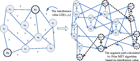
Example of calculating the augment paths
Full size image

3)
Finding an augment path

Finding the augment path is a key step in obtaining k _ij node-disjoint paths. As showed in Fig. 4, the augment path is marked by a dotted line. Specifically, in Fig. 4, the source and destination are, respectively, v ₁ and v ₉. As long as v ₉ is selected as a node in the minimum spanning tree (MST) found based on the links weight LIS(G), the calculation of the augment path is achieved, and the algorithm enters next step.

4)
Updating link capacity on augment path

After calculating the augment path, the unit capacity of directed link is updated. For example, in Fig. 5, for the link (v ₁”, v ₅’), c(v ₁”, v ₅’) = c(v ₁”, v ₅’)-1 = 0, and c(v ₅’,v ₁”) = c(v ₅’,v ₁”) + 1 = 1, the link changes to the reverse direction. The other links on the augment path execute the same operation.
Fig. 5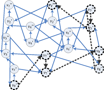
Example of updating the capacity of link
Full size image

5)
Merging the augment path to the output topology

When the number of augment paths is not less than k _ij, the disjoint paths between v _i and v _j are found. In this context, we need to merger the augment path into the output topology. As shown in Fig. 6, the two augment paths between v ₁ and v ₈ are added into the output topology.
Fig. 6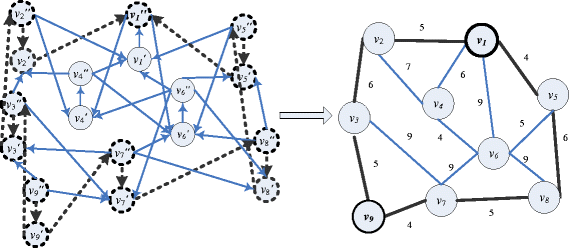
Example of merging the augment paths
Full size image

Main procedure is summarized in Algorithm 1.

Theoretical analysis of the proposed FICTC

To identify the theoretical performance of FICTC, we present some theorems to prove the performance.

Theorem 1

Give a network G(V,E), let v _x,v _y as two different nodes in G(V,E) the min-edge-cut set between v _x and v _y is equivalent to the maximum integer flow in unit capacity network.

Proof

From max-flow min-cut theorem, the maximum flow between v _x and v _y is equal to the sum capacity of the minimum cut edge set. In addition, the maximum capacity is equal to the number of the minimum cut edge set, when the network is with unit capacity. In a unit capacity network, the capacity of each edge is 1; hence, the min-cut set between v _x and v _y is equivalent to the maximum integer flow in a unit capacity network.

Theorem 2

Given a network G(V,E), let v _x,v _y as two different nodes in G(V,E) the number of node-disjoint paths is equal to the maximum integer flow in a unit capacity network obtained by the node-splitting technique.

Proof

From Menger’s theorem [34], the number of node-disjoint paths between any two nodes is equal to that of minimum vertex separation. Since the network is unit capacity obtained by node-splitting, the number of minimum vertex separation is equal to the minimum edge cut set obtained via Theorem1. Thus, we prove the theorem.

Theorem 3

Given an initial network G(V,E), the maximum link interference of the topology G _d(V’,E’) constructed by the proposed FICTC is minimized.

Proof

Suppose G(V,E) meet the fault-tolerant constraint. According Section 6, FICTC achieves the optimal topology via node-disjoint paths set R between any two nodes, which are obtained by Prim’s minimum span tree algorithm. If we can prove the link maximum interference in path P∈R in G _d(V',E') is minimized, we can conclude that the result is true.

Now, we prove by contradiction that each node-disjoint path P in G _d(V’,E’) is minimized. Let T be the minimum span tree and P be a augment path between v _x and v _y, where P∈T and P∈R. Assume the link maximum interference in path P in G _d(V’,E’) is not minimized. Then, there exist links e and e’, where e∈E(T), e’∈E(G-T), LIS(e’) < LIS(e), and LIS(P- e + e’) = LIS(P) -LIS(e) + LIS(e’) < LIS(P). Since P∈T and there is only one path between any two nodes in T, the number of paths between v _x and v _y is 1. Hence, LIS(T- e + e’) = LIS(T) -LIS(e) + LIS(e’) < LIS(T) leads to a contradiction.

Then, we analyze the computational complexity of FICTC. For a given G(V,E) with n nodes and m links, we use a adjacency list to store the network graph G(V,E). Consider the gateway node already collects all node information. FICTC mainly includes procedures of splitting operation and seeking the k _ij disjoint paths between v _i and v _j. For the procedures of splitting operation, v _i is replaced with v _i ’ and v _i ” and each link is replaced with two directed link e’ = (v _i”, v _j’) and e” = (v _j”, v _i’), and the total time complexity is O(n + m). In procedure for seeking the k _ij disjoint paths, since the network includes n(n-1)/2 different node pairs, the time of solving k _ij node-disjoint paths are n(n-1)/2. For each procedure of solving k _ij node-disjoint paths, it needs to compute k _ij node-disjoint paths. In the process of computing, an augment path between any two nodes is found by Prim’s minimum spanning tree algorithm. If the graph G(V,E) is stored in the adjacency list, the complexity of Prim’s minimum spanning tree algorithm is O(m + n). After finding the augment paths, these paths are used to update the flow. The flow updating of each path in worst case take n-1 times addition operation and subtraction operation, then the total time of finding the k _ij augment paths is O(k _ij n). k _ij is various for different node pairs; we thus use max(k _ij) to represent it. Therefore, the total computational complexity of FICTC is O(2n(n-1) max(k _ij) (m + n + k _ij n)).

Distributed implementation of the proposed FICTC

In wireless multi-hop network, the practical implementation is generally in a distributed way. In this section, we present the distributed implementation of the proposed FICTC.

The topology of distributed implementation is derived by its neighbor nodes’ information of each node. The implementation procedure includes three phases. In first phase, each node v first calculates the interference level ULIS(v, u) based on locally collected neighbor information and the formula (2) in section 3.2. Then, each node sent their the interference level ULIS(v, u) to their neighbor nodes. Finally, according to the formulas (3) and (4), each node calculate the LIS(u, v) based on ULIS(u, v) and the received ULIS(v, u) from their neighbor nodes. In second phase, according to the k _ij connectivity fault-tolerant requirement, the k _ij disjoint paths between any two nodes pair are required to be solved in disturbed way. Therefore, in the process of solving k _ij disjoint paths, the augment path is achieved based on distributed minimum spanning tree (MST) algorithm [35]. In the final phase, these links that included in all augment paths are merged into the constructed topology. The detailed procedure is summarized in Algorithm 2.

Performance evaluation

First, we take an example to detail FICTC and compare with other k-connected algorithms, such as FLSS and LTRT. Consider a network with 50 nodes randomly placed in a 1000 m × 1000 m field; transmit range of all nodes is 250 m. We randomly generate 10 nodes and assume that the fault-tolerant constraints k _ij among them are 3, and that among others nodes are 2, i.e., N _fl(v _i,v _j) ≥ 3, i,j∈{0,4,7,8,15,18,25,35,37,43}, i ≠ j, and N _ft(v _i’,v _j’) ≥2, i',j’∈{V-{0,4,7,8,15,18,25,35,37,43}}, i' ≠ j’. The topologies constructed by UDG, FLSS, LTRT, and FICTC are respectively shown in Fig. 7a–d.

From Fig. 7, Fig. 7a is original topology constructed by unit disk graph (UDG), i.e., unit disk graph is a network topology derived by using the maximum the transmission radius of 250 m. In Fig. 7b, the topology constructed by the FLSS algorithm. This algorithm first sorts all edges in ascending order of weight, then judges the k-connected between two terminate nodes of each edge in the order. If it is k-connected, the edge is inserted into output topology graph G _k. For the topology derived by LTRT in the Fig. 7(c), the LTRT algorithm is a topology control algorithm combining two different algorithms, TRT and LMST. TRT is basically an algorithm to efficiently construct 2-edge connected topologies. However, it can be extended for constructing k-edge connected networks by just recursively repeating the same procedures. The topology constructed by our proposed FICTC is shown in Fig. 7d. In Fig. 7, our proposed FICTC shows the number of disjoint paths between any node pair in 10 nodes {0,4,7,8,15,18,25,35,37,43} is 3, while others are 2, showing the constructed topology satisfies the specific fault-tolerant requirement k _ij. Furthermore, we can easily know from Fig. 7, the FICTC present smaller transmit radius and node degree than FLSS and LTRT. The performance of FLSS is better than LTRT.

Then, in order to show the validation of our proposed algorithm, we consider a network with 50 to 100 nodes randomly placed in a 1000 m × 1000 m field. Transmission range of all nodes is 250 m. Table 1 lists the fault-tolerant requirement. The nodes are divided into two groups. We compare our FICTC with FLSS and LTRT. The graph parameters of comparison among FLSS, LTRT, and FICTC include node degree and transmit radius. The node degree is referred as the number of nodes within the transmission radius of a node. Figures 8, 9, and 10 demonstrate a comparison among these topology control algorithms. Here, the NONE denotes the original topology constructed by UDG in Figs. 8, 9, and 10.

Table 1 Simulation parameters setting

Full size table

Figure 8 shows the average node degree of the topologies derived by FLSS, LTRT, FICTC, and NONE. The NONE in Fig. 8 is defined as the network topology derived by using the maximum transmit radius. The node degree of NONE linearly increases with the number of nodes, while node degrees of FLSS, LTRT, and FICTC are almost constant. Meanwhile, the average node degree of FICTC is smaller than other algorithms. In Fig. 8b, the average transmit radius of FICTC is smaller than FLSS, LTRT, and NONE, indicating better network performance in terms of interference.

But, as we know from [32], the minimum node degree does not imply the minimum interference. In order to further validate the performance of total interference, we evaluate the performance of our proposed algorithms in above random network using the interference metric in section 3.2. In Fig. 9, we plot respectively the maximum links interference and average links interference for a varying number of nodes.

Figure 9 shows FICTC and distributed FICTC enjoy better maximum link interference performance over FLSS, LTRT, and NONE. Meanwhile, in Fig. 9b, the average link interference of FICTC is weaker than NONE, LTRT, and FLSS. Since FICTC considers the interference metric as link cost, thus we can achieve the minimal of maximum interference.

Then, we evaluate the average expended energy ratio (EER), where is defined in [13, 14]. The definition is as follows.

$$ EER={E}_{\mathrm{AVE}}\div {E}_{\mathrm{MAX}}\times 100\left[\%\right] $$

(8)

In (8), the E _AVE denotes the average transmission power over all the nodes, and E _MAX is the maximal transmission power. We compare the EER performance of our FICTC with FLSS and LTRT. The result of performance is shown in Fig. 10.

In Fig. 10, we know the proposed FICTC and distributed FICTC both performs better than other algorithms and the difference of performance reduce with the increase of the number of nodes.

In order to fully understand FICTC, we evaluate the performance of different algorithms by ns-2 simulations. The parameters are shown in Table 2. We utilize UDP connection and constant bit rate (CBR) flow for each pair. The length of packet is 512 bytes and the sending rate of each CBR flow is fixed at 2 Mbps. All transmissions are unicast following the 802.11 MAC protocol. The routing scheme is AODV for MCMR-WMN. As for the fault-tolerant requirements, we use UDG, FLSS, LTRT, distributed FICTC, and FICTC. We compare the performance by measuring the throughput and average E2E delay.

Table 2 Simulation parameters

Full size table

Figure 11 shows that the throughput of FICTC and distributed FICTC are higher than NONE, LTRT, and FLSS; meanwhile, its average E2E delay is the lowest. Unlike FLSS and LTRT, FICTC not only considers the length of the shortest path, but also uses the link interference as link weight in solving the topology. Importantly, only FICTC achieves the fault-tolerant constraint between any two nodes.

Conclusions

In this work, topology optimization of considering the fault tolerance and network interference in WNMs was investigated. We proposed a fault-tolerance-and-interference-aware topology control (FICTC) algorithm for WNMs. We first analyzed the network performance under the requirement of k-connectivity. Then, the interference model and the problem formulation of improving the network performance for k-connectivity topology were presented. By the analysis of FICTC algorithm, we proved that FICTC not only meets the fault-tolerant requirement, but also minimizes the maximum node interference. Moreover, the distributed implementation of the proposed FICTC was proposed. The proposed FICTC algorithm plays an important role for improving network and fault tolerance performance in WNMs. We integrate the disjoint paths between any two nodes into topology optimization with fault tolerance requirement. For different fault tolerance requirement, graph-based simulations results indicated that FICTC outperforms the state-of-the-art fault-tolerant topology control algorithms in terms of average node degree, maximum transmit radius, and maximum link interference. Furthermore, the ns-2 simulations showed FICTC achieves higher throughput and lower E2E delay. In term of energy consumption, we use the average expended energy ratio (EER) to evaluate the energy performance of our proposed FICTC. The result indicated the proposed FICTC achieve lower EER than other algorithms. These results demonstrate that the proposed solutions are promising for specific fault-tolerant requirement in practical network deployment. However, There are several problems for further research on fault-tolerance-and-interference-aware topology control. The proposed FICTC does not analyze the network performance of considering sophisticated model for the radio signal propagation. Moreover, the FICTC algorithm needs to deal with mobile WNMs. In future study, we plan to investigate the network performance for these problems.

References

1.
M Li, Z Li, AV Vasilakos, A survey on topology control in wireless sensor networks: taxonomy, comparative study, and open issues. Proceedings of the IEEE 101(12), 2538–2557 (2013)
Article Google Scholar
2.
J Gui, Z Zeng, Joint network lifetime and delay optimization for topology control in heterogeneous wireless multi-hop networks. Comput. Commun 59, 24–36 (2015)
Article Google Scholar
3.
X Chu, H Sethu, An Energy Balanced Dynamic Topology Control Algorithm for Improved Network Lifetime. 2014 IEEE 10th International Conference on Wireless and Mobile Computing, Networking and Communications (WiMob), 2014, pp. 556–561
Google Scholar
4.
M Abbasi, N Fisal, Noncooperative game-based energy welfare topology control for wireless sensor networks. IEEE sensors J 15(4), 2344–2355 (2015)
Article Google Scholar
5.
YH Liu, Q Zhang, LM Ni, Opportunity-based topology control in wireless sensor networks. IEEE Trans. Parallel Distrib. Syst 21(3), 405–416 (2010)
Article Google Scholar
6.
MR Rai, S Vahid, K Moessner, SINR Based Topology Control for Multihop Wireless Networks With Fault Tolerance. Proceedings of 2015 IEEE 81st Vehicular Technology Conference (VTC Spring), 2015, pp. 1–6
Google Scholar
7.
M Haghpanahi, M Kalantari, M Shayman, Topology control in large-scale wireless sensor networks: between information source and sink. Ad Hoc Networks 11(3), 975–990 (2013)
Article Google Scholar
8.
AA Jeng, RH Jan, Adaptive topology control for mobile ad hoc networks. IEEE Trans. Parallel Distrib. Syst 22(12), 1953–1960 (2011)
Article Google Scholar
9.
A Vázquez-Rodas, L Llopis, A centrality-based topology control protocol for wireless mesh networks. Ad Hoc Networks 24, 34–54 (2015)
Article Google Scholar
10.
F Senel, K Akkaya, M Erol-Kantarci et al., Self-deployment of mobile underwater acoustic sensor networks for maximized coverage and guaranteed connectivity. Ad Hoc Networks 34, 170–183 (2015)
Article Google Scholar
11.
XM Zhang, Y Zhang, F Yan, A Vasilakos, Interference-based topology control algorithm for delay-constrained mobile ad hoc networks. IEEE Trans. Mobile Comput. 14(1), 742–754 (2015)
Article Google Scholar
12.
DM Blough, M Leoncini, G Resta et al., The k-neighbors approach to interference bounded and symmetric topology control in ad hoc networks. IEEE Trans. Mobile Comput 5(9), 1267–1282 (2006)
Article Google Scholar
13.
N Li, JC Hou, Localized fault-tolerant topology control in wireless ad hoc networks. IEEE Trans. Parallel Distrib. Syst 7(4), 307–320 (2006)
Article Google Scholar
14.
K Miyao, H Nakayama, N Ansari, LTRT: an efficient and reliable topology control algorithm for Ad-Hoc networks. IEEE Trans. Wireless Commun 2(8), 6050–6058 (2009)
Article Google Scholar
15.
X Wang, M Sheng, M Liu et al., RESP: A k-Connected Residual Energy-Aware Topology Control Algorithm for Ad Hoc Networks. 2013 IEEE Wireless Communications and Networking Conference (WCNC), 2013, pp. 1009–1014
Google Scholar
16.
H Bagci, I Korpeoglu, A Yazici, A distributed fault-tolerant topology control algorithm for heterogeneous wireless sensor networks. IEEE Trans. Parallel Distrib. 26(4), 914–923 (2014)
Article Google Scholar
17.
J Zhao, G Cao, Robust topology control in multi-hop cognitive radio networks. IEEE Trans. Mobile Comput. 13(11), 2634–2647 (2014)
MathSciNet Article Google Scholar
18.
S Gundry, J Zou, J Kusyk, CS Sahin, MU Uyar, Differential Evolution Based Fault Tolerant Topology Control in MANETs. 2013 IEEE Military Communications Conference, 2013, pp. 864–869
Google Scholar
19.
J Guo, X Liu, C Jiang, J Cao, Y Ren, Distributed fault-tolerant topology control in cooperative wireless ad hoc networks. IEEE Trans. Parallel Distrib. Syst. 26(10), 2699–2710 (2015)
Article Google Scholar
20.
X Ao, FR Yu, S Jiang, Q Guan, VCM Leung, Distributed cooperative topology control for WANETs with opportunistic interference cancelation. IEEE Trans. Veh. Technol. 63(2), 789–801 (2014)
Article Google Scholar
21.
C Luo, G Min, FR Yu, M Chen, LT Yang, VCM Leung, Joint topology control and authentication design in mobile ad hoc networks with cooperative communications. IEEE J. Sel. Areas Commun 61(6), 2674–2685 (2012)
Google Scholar
22.
T Fukunaga, Z Nutov, R Ravi, Iterative rounding approximation algorithms for degree-bounded node-connectivity network design. SIAM J. Comput 44(5), 1202–1229 (2015)
MathSciNet Article MATH Google Scholar
23.
L Li, YH Joseph, B Paramvir et al., A cone-based distributed topology-control algorithm for wireless multi-hop networks. IEEE/ACM Trans. Netw 13(1), 147–159 (2005)
Article Google Scholar
24.
Q Guan, FR Yu, S Jiang, VCM Leung, H Mehrvar, Topology control in mobile ad hoc networks with cooperative communications. IEEE Wireless Commun. Mag. 19(2), 74–79 (2012)
Article Google Scholar
25.
K Xu, M Gerla, S Bae, How Effective is the IEEE 802.11 RTS/CTS Handshake in ad hoc Networks. IEEE Global Telecommunications Conference, 2002, pp. 72–76
Google Scholar
26.
M Burkhart, P Rickenbach, R Wattenhofer et al., Does Topology Control Reduce Interference? Proceedings of 5th ACM International Symposium on Mobile Ad Hoc Networking and Computing (MobiHoc’04), 2004, pp. 9–19
Google Scholar
27.
Z Xu et al., Crowdsourcing based Social Media Data Analysis of Urban Emergency Events. Multimedia Tools and Applications. doi:10.1007/s11042-015-2731-1
28.
Z Xu et al., Crowdsourcing based Description of Urban Emergency Events using Social Media Big Data. IEEE Transactions on Cloud Computing. doi:10.1109/TCC.2016.2517638
29.
Z Xu, H Zhang, V Sugumaran, K Choo, L Mei, Y Zhu, Participatory sensing-based semantic and spatial analysis of urban emergency events using mobile social media. EURASIP Journal on Wireless Communications and Networking 2016, 44 (2016)
Article Google Scholar
30.
P Gupta, PR Kumar, The capacity of wireless networks. IEEE Trans. Inf. Theory 46(2), 388–404 (2000)
MathSciNet Article MATH Google Scholar
31.
S Ji, Z Cai, Distributed data collection in large-scale asynchronous wireless sensor networks under the generalized physical interference model. IEEE/ACM Transactions on Networking 21(4), 1270–1283 (2013)
Article Google Scholar
32.
ME Haque, A Rahman, Fault Tolerant Interference-Aware Topology Control for Ad Wireless Networks. ADHOC-NOW'11: Proceedings of the 10th international conference on Ad-hoc, mobile, and wireless networks, 2011, pp. 100–116
Google Scholar
33.
R Hekmat, P Van Mieghem, Interference in wireless multi-hop ad-hoc networks and its effect on network capacity. Journal Wireless Networks 10(4), 389–399 (2004)
Article Google Scholar
34.
T Böhme, F Göring, J Harant, Menger’s theorem. Journal of Graph Theory 38(1), 35–36 (2001)
Article MATH Google Scholar
35.
K Maleq, P Gopal, A fast distributed approximation algorithm for minimum spanning trees. Distributed Computing 20(6), 391–402 (2008)
Article MATH Google Scholar

Download references

Acknowledgements

This research was supported by the National Natural Science Fund of China (Grant No. 61401189), Natural Science Foundation of Jiangxi, China (Grant No. 20161BAB212036), Natural Science Fund of Nanchang Institute of technology (No.2014KJ016), and the Science and Technology Plan Project of the Education Department of Jiangxi Province of China (GJJ14751).

Competing interests

The authors declare that they have no competing interests.

Authors’ information

Xuecai Bao received Ph.D. degree from school of electronics and information engineering at Harbin Institute of Technology, Harbin, People’s Republic of China. He is currently a lecturer in the Jiangxi Province Key Laboratory of Water Information Cooperative Sensing and Intelligent Processing, Nanchang Institute of Technology, Nanchang. His research interests include resource management for wireless mesh networks, wireless ad hoc networks, and wireless sensor network.

Chengzhi Deng received the M.S.c degree in Optics from Jiangxi Normal University, Nanchang, China, in 2005, and the Ph.D degree in information and communication engineering from Huazhong University Science and Technology, Wuhan, China in 2008. He is currently a professor in the Jiangxi Province Key Laboratory of Water Information Cooperative Sensing and Intelligent Processing, Nanchang Institute of Technology, Nanchang. His major research interests focus on wireless sensor network, image reconstruction, and remote sensing image processing.

Author information

Affiliations

Jiangxi Province Key Laboratory of Water Information Cooperative Sensing and Intelligent Processing, Nanchang Institute of Technology, 330099, Nanchang, Jiangxi, China
Xuecai Bao & Chengzhi Deng
School of Information Engineering, Nanchang Institute of Technology, 330099, Nanchang, Jiangxi, China
Xuecai Bao & Chengzhi Deng

Authors

Xuecai Bao
View author publications
You can also search for this author in PubMed Google Scholar
Chengzhi Deng
View author publications
You can also search for this author in PubMed Google Scholar

Corresponding author

Correspondence to Xuecai Bao.

Rights and permissions

Open Access This article is distributed under the terms of the Creative Commons Attribution 4.0 International License (http://creativecommons.org/licenses/by/4.0/), which permits unrestricted use, distribution, and reproduction in any medium, provided you give appropriate credit to the original author(s) and the source, provide a link to the Creative Commons license, and indicate if changes were made.

Reprints and Permissions

About this article

Cite this article

Bao, X., Deng, C. FICTC: fault-tolerance-and-interference-aware topology control for wireless multi-hop networks. J Wireless Com Network 2016, 190 (2016). https://doi.org/10.1186/s13638-016-0690-5

Download citation

Received: 21 May 2016
Accepted: 09 August 2016
Published: 19 August 2016
DOI: https://doi.org/10.1186/s13638-016-0690-5

Keywords

Interference-aware topology control
Fault-tolerance constraints
Wireless multi-hop network

FICTC: fault-tolerance-and-interference-aware topology control for wireless multi-hop networks

Abstract

Introduction

Related work

Related model and problem formulation

Network model

Interference model

Problem formulation

Fault-tolerance-and-interference-aware topology control

Description of FICTC algorithm

Theoretical analysis of the proposed FICTC

Theorem 1

Proof

Theorem 2

Proof

Theorem 3

Proof

Distributed implementation of the proposed FICTC

Performance evaluation

Conclusions

References

Acknowledgements

Competing interests

Authors’ information

Author information

Affiliations

Corresponding author

Rights and permissions

About this article

Cite this article

Keywords