- Research
- Open access
- Published:
Suppression of multiple wideband interferences based on superposition probability
EURASIP Journal on Wireless Communications and Networking volume 2016, Article number: 198 (2016)
Abstract
Superposed multicarrier transmission is one of the schemes that achieve efficient use of frequency resources. In the scheme, desired signals are interfered by other systems sharing the same frequency band, which causes unreliable LLR (log-likelihood ratio) setting and leads to degradation of the BER (bit error rate) performance. In many conventional schemes for OFDM (orthogonal frequency division multiplexing) systems, the interference power for each subcarrier is estimated independently. Otherwise, based on the assumption that interferences have the same average power, one interference power is estimated and applied to all subcarriers. However, when there exist multiple wideband interferences with different average power, it is better to detect each interference and estimate each power based on all subcarriers within each superposed band to make it accurate. In this paper, we propose a scheme to suppress multiple wideband interferences based on the probability with which each subcarrier is superposed, referred to as the superposition probability. In the proposed scheme, we derive the PDFs (probability density functions) of residual powers for superposed and non-superposed bands. Based on residual powers and their PDFs, we calculate the superposition probability for each subcarrier. Furthermore, we perform superposed band detection iteratively according to the probabilities and update each estimated interference power. Through simulations, we show that the detection rate of superposed bands is improved by iterating superposed band detection based on superposition probabilities. We also show that the proposed scheme achieves the better BER performance than that of conventional ones.
1 Introduction
Rapid increase of wireless communication systems and growing demand for high-speed communication have brought about lack of frequency resources [1]. One of the techniques that realize efficient use of frequency resources is spectrum sharing where several wireless systems share the same spectrum to make overall occupied frequency band narrower [2]. Superposed multicarrier transmission is one of the spectrum sharing schemes, which allows the occupied band of unexpected signals to overlap a part of the occupied one of the desired signals [3, 4]. However, desired signals on the superposed bands are affected by other systems that use the same frequency bands. Those interferences cause unreliable LLR (log-likelihood ratio). Because LLR is a metric for decoders, inaccurate LLR makes BER (bit error ratio) performance degrade. Because interference parameters, like power and occupied bands, are usually not available, interferences should be detected and also suppressed at the receiver side by any information obtained from received signals.
A lot of schemes of interference suppression for OFDM (orthogonal frequency division multiplexing) systems are proposed over the past years. For example, in cognitive radio OFDM systems, unlicensed users are allowed to use the licensed bands where the licensed users are not present. Though OFDM subcarriers are orthogonal to each other, each subcarrier has high sidelobes, which is one of the crucial problems to be solved. In [5, 6], AIC (active interference cancellation) is used for sidelobe suppression. In [5], extended AIC signals are added to suppress sidelobes and to shape the spectrum of OFDM signal with a CP (cyclic prefix). In the scheme, the extended AIC signal with CP employs cancelation signals composed of tones spaced closer than the interval of OFDM subcarriers to cancel the sidelobes of OFDM signals. In addition, optimal cancelation signals are derived to minimize the total power of sidelobes. In [6], the problem of spectrum overshooting is coped with by employing the improved AIC technique. In the scheme, a trade-off between the amount of spectrum overshooting and sidelobe suppression without increasing the computational complexity is obtained by solving the optimizing problem in AIC; the influence of spectrum overshooting can be totally removed.
In [7, 8], null symbols are transmitted at a constant interval for spectrum sensing. Though they are some overhead for systems, it is simple with respect to implementation. In [9], a prediction-error filter is employed to detect narrow-band interferences, and then, erasure insertion is performed over the detected superposed bands. Similarly, in [10], hidden Markov model-based filters and smoothers are employed for dynamic excision of narrow-band interferences from spread-spectrum systems. In [11], the interference power of each subcarrier is estimated based on previous decoded data in the same packet. In the scheme, it is necessary to insert more pilot signals for initial estimation of the interference power than those just required to estimate channel coefficients, which are large overhead for systems. To reduce this overhead, another scheme is proposed in [12], which applies EM (expectation maximization) algorithm for estimation of the interference power of each subcarrier. EM algorithm is a kind of the maximum likelihood estimation schemes that calculates local optimum parameters of a stochastic model based on given initial parameters. In addition, an approach using the EM algorithm is applied to address the frequency estimation problem in OFDM spectrum sharing systems [13] and to estimate channel coefficients [14]. Through simulations, it is shown that nearly the same BER performance as that in [11] is achieved with less amount of overhead, while computational complexity increases due to iterative Viterbi decoding in the loop of EM algorithm. In [15], estimation of an interference power and decoding of received signals are alternately performed. At the receiver side, at first, robust LLR is calculated for initial decoding. Exploiting LLR output from the decoder, soft-decision replica signals are generated to calculate residual powers. Comparing them with a threshold power, superposed bands and an interference power are estimated. Based on the estimated parameters, LLR calculation and decoding are performed again. Repeating the process, accuracy of the estimation increases. One drawback of the scheme is large computational complexity because of iterative decoding. In [16], EM algorithm is applied to reduce the computational complexity. At the receiver side, first, residual powers are calculated by exploiting hard-decision replica symbols. Based on the residual powers, an interference power and superposed rate are iteratively estimated in the EM algorithm. Superposed rate is defined as a ratio of the number of subcarriers on superposed bands to the number of those composing an OFDM symbol. This scheme can achieve the BER performance close to that in [15] with one decoding iteration.
In [15, 16], the average power of each interference is assumed to be equal as shown in Fig. 1. In practice, however, multiple interferences with different average power can exist as shown in Fig. 2. Considering that case into account, we proposed an interference suppression scheme that can be applied to the both cases where the interference power is equal or different [17]. In the scheme, residual powers are averaged in both time and frequency domains to mitigate the variance of them among subcarriers on the same superposed band. Besides, the threshold used to detect superposed bands is updated according to the equation proposed in [16] and superposed band detection is iteratively performed. Although the BER performance is slightly improved compared to that of conventional schemes for large E b /N 0, and also, the detection rate of superposed bands is made higher by updating the threshold, there are still several points to be improved. One of them is how to calculate LLR. In [17], each estimated interference power is never exploited to calculate LLR for non-superposed bands. However, even for subcarriers detected as non-superposed bands, we should take the possibility of their belonging to superposed bands into account according to the magnitude of each residual power. One of the possible ways is to calculate LLR weighted with the probability with which each subcarrier is superposed, which is referred to as “superposition probability” in this paper. The other point is related to the way to calculate the threshold power. The equation for optimizing the threshold is derived on the assumption that all interference power is equal. Therefore, the threshold is hard to be optimized when the interference power is different, like under the interference scenario in Fig. 2.

Interference model assumed in conventional schemes

Interference model assumed in the proposed scheme
In this paper, we propose a scheme to suppress multiple independent wideband interferences with different power based on superposition probabilities. In the proposed scheme, in accordance with the PDFs (probability density functions) of residual powers for superposed and non-superposed bands, we derive equations that give superposition probabilities for both the pilot part and data part in a packet. We iterate superposed band detection by updating not the threshold but the superposition probability. Besides, the proposed scheme needs no information about interferences as well as the noise power. Through simulations, we show that the detection rate of superposed bands is significantly improved by exploiting superposition probabilities. We also show that the BER performance is greatly improved compared to that of conventional schemes in the presence of several wideband interferences with different power. As one reason for the improvement, we evaluate accuracy of each estimated interference power by NRMSE (normalized root-mean-squared error).
The rest of this paper is organized as follows. Section 2 specifies the system model. Section 3 introduces how to estimate initial noise and interference power with pilot OFDM symbols and defines the superposition probability. Section 4 introduces iterative superposed band detection scheme with data OFDM symbols. In Section 5, we show simulation results for several interference scenarios, which is followed by the conclusion in Section 6.
2 System model
We suppose an OFDM (orthogonal frequency division multiplexing) system with single transmit and receive antennas. Each OFDM symbol is composed of L subcarriers and contains FEC (forward error correction) codes generated by a turbo encoder. At the receiver side, GI (guard interval) is removed and FFT (fast Fourier transform) is applied to received OFDM symbols to transform those from time domain into frequency domain. We assume that we can obtain perfect time and frequency synchronization. Then, a received OFDM symbol at time t, subcarrier index l (0≤l≤L−1) is expressed as
where h(t,l),x(t,l),n(t,l), and w(t,l) represent channel coefficient, transmitted signal, noise signal, and interference signal, respectively. We assume that each n(t,l) is a circularly symmetric complex Gaussian random variable with mean 0 and variance \({\sigma _{n}^{2}}\). We also assume that I independent wideband interferences are superposing on desired OFDM symbols. The prefix “wideband” means that each interference is assumed to superpose over several consecutive subcarriers of the desired OFDM symbol in frequency domain. Note that the wideband interferences do not overlap each other. We denote their indices by i, the set of indices of subcarriers superposed by the wideband interference i by l i , and the set of indices of subcarriers on non-superposed bands by \(\overline {\mathbf {l}}\), respectively. Then, w(t,l) is a part of the wideband interference i (l∈l i ) and is corresponding to the subcarrier l of the desired OFDM symbol. We also assume that w(t,l) for each subcarrier l is modeled as an independent, circularly symmetric complex Gaussian random variable with mean 0 and variance \(\sigma _{\text {if}}^{2}(l)~=~\sigma _{\text {if},i}^{2}(l\in \mathbf {l}_{i})\), where w(t,l) = 0 for \(l\in \overline {\mathbf {l}}\). Namely, all w(t,l) belonging to the same wideband interference i have the same variance \(\sigma _{\text {if},i}^{2}\). Note that the wideband interference has to be modeled properly, based on, for example, modulation scheme, the channel between the desired receiver and the transmitter of interference signals, and nonlinearity of the desired receiver.
In this paper, we consider the environment where coordinated and unknown systems may be present. In other words, there is no priority and no cooperation among systems. Therefore, the bands used by other radio systems can be anywhere in the desired bands. Also, the power of interference signals transmitted by other radio systems can be smaller or larger than that of the desired signal. In addition, the power spectral density of each interference is assumed to be constant at passband with steep slopes. In the following, we omit the part “wideband” and just describe “interference i” to be simplified.
A packet is composed of Q pilot OFDM symbols known to the receiver followed by K data OFDM symbols. We assume that the channel is time-invariant but frequency selective during the reception of a packet. Also, we assume that the interference signal lasts long enough to state that it does not start or end during the reception of a packet. Moreover, the superposed band and the power of each interference is constant in each packet. Although the main purpose of inserting pilot OFDM symbols is to estimate channel coefficients, in addition to channel estimation, we exploit them to estimate noise and interference power based on the technique proposed in [18].
We first estimate the channel coefficient for each subcarrier with pilot OFDM symbols. In the pilot part, a received pilot signal is expressed as
where superscript P indicates that it is related to pilot OFDM symbols. x P(t,l) is any of the candidate symbols in M-PSK or M-QAM. We obtain the channel coefficients simply in the following.
where (·)∗ is the complex conjugate of (·). In practice, the channel estimation error affects the accuracy of superposed band detection or the BER performance.
The LLR of the mth bit c(t,l,m) of the transmitted data OFDM symbol at time t and subcarrier index l is given by
where P(·) is the probability. Since interference parameters are usually unknown to the receiver, robust LLR is proposed in [19], which weights two PDFs by a coefficient to take interferences into account. As robust LLR is tolerant toward variation of interference parameters, in [15, 19], the interference power and the coefficient are set to 4 and 0.3, respectively, as constant values. However, there are some points to be mentioned. First, the noise power has to be known. Second, applying the same coefficient to all subcarriers is not optimal. In other words, a different coefficient should be chosen for each subcarrier based on any information obtained from received OFDM symbols. Thus, we exploit the pilot OFDM symbols to combat these problems. Specifically, we calculate subtraction of two pilot OFDM symbols consecutive in time domain and derive its PDFs. Based on the magnitude of the subtraction, we detect superposed bands and estimate noise and interference power. Moreover, we calculate superposition probabilities, which is denoted by P if(l) in the following, based on the obtained PDFs to be utilized for LLR calculation.
3 Initial estimation of noise and interference power with pilot OFDM symbols
We show the proposed receiver structure in Fig. 3. In this section, we show the way to obtain initial estimators \(\hat {\sigma }_{n}^{2}, \hat {\sigma }_{\text {if}}^{2}\), and \(P_{\text {if}}^{\mathrm {P}}(l)\) by exploiting pilot OFDM symbols. In Fig. 3, the upper detector, “Initial detector,” corresponds to the estimation in this section. For simplicity, here, we assume the number of pilot OFDM symbols Q = 2 and denote them by y(0,l),y(1,l), respectively. Assuming that channel coefficients of two pilot signals consecutive in time domain are approximately equal, the subtraction r P(l) of them can be expressed as

Proposed receiver structure
where H 0 and H 1 represent the hypotheses of being on a non-superposed and a superposed band, respectively. Denoting the in-phase and quadrature components of n(k,l) and w(k,l) by n I(k,l), n Q(k,l), and w I(k,l),w Q(k,l), respectively, |r P(l)|2 is expressed as follows.
For each component X(= I, Q), we can easily find that,
From Eqs. (6) and (7), |r P(l)|2 is χ 2 distributed with D = 2 degrees of freedom. For statistically independent and identically distributed Gaussian random variables X j (j = 0,1,…,D − 1) with mean 0 and variance σ 2, the PDF of \(Z~=~\sum _{j~=~0}^{D-1}{X_{j}^{2}}\), represented by p(z), is expressed as follows.
where Γ(·) is the Gamma function. Hence, the PDFs of z P(l)≡|r P(l)|2 for H 0 and H 1 are given, respectively, as,
Here, we set a threshold \(|r_{\text {th}}^{\mathrm {P}}|^{2}\) to be compared with z P(l) to estimate subcarriers affected by interferences. Because we do not have any information about interferences at this stage, we set the average of all z P(l) to the threshold. That is,
Each z P(l) is compared with \(|r_{\text {th}}^{\mathrm {P}}|^{2}\). Namely,
Note that for H 1 in Eq. (5), w(0,1)−w(1,l) may be zero or very small compared to n(0,l)−n(1,l). In this case, the decision in Eq. (11) may get wrong because the corresponding z P(l) is not so large compared to that on non-superposed bands.
Denoting the set of subcarrier indices on detected superposed and non-superposed bands by l and \(\overline {\mathbf {l}}\), respectively, noise and interference power are obtained by averaging z P(l) within l and \(\overline {\mathbf {l}}\). That is,
Because in the previous section we assumed that each interference superposes on at least two consecutive subcarriers of the desired OFDM symbols in frequency domain, we can estimate each interference power accurately by averaging procedure in Eq. (12). Note that the proposed scheme can work in the case where there exist interferences superposing on just one subcarrier of the desired OFDM symbol. Based on Eq. (9) and estimated parameters in Eq. (12), we derive the superposition probability \(P_{\text {if}}^{\mathrm {P}}(l)\). Taking the integral of the PDF p(z|H) with respect to zgives P(z|H), which is the probability with which z is obtained for the hypothesis H. Specifically, the integral of p P(z P(l)|H 0) and p P(z P(l)|H 1) with respect to z P(l) corresponds to the probability P(z P(l)|H 0) and P(z P(l)|H 1), respectively. For this reason, we consider the ratio of the probability for H 1 to the sum of that for H 0 and H 1, as the superposition probability. Namely,
where z P(l)≡|r P(l)|2. Note that this scheme can work for any value of Q≥2. Let \(\mathbf {Y}^{\mathrm {P}}(l)=\{y^{\mathrm {P}}({i,l})\}_{i=0}^{Q-1}\) be the set of pilot OFDM symbols for the subcarrier l in a packet. Then, we obtain Q − 1 subtractions from Y P(l), defined as r P(i,l), as follows.
Letting z P(i,l)≡|r P(i,l)|2, we replace z P(l) with \(\mathbb {E}[\!z^{\mathrm {P}}({i,l})]_{i}\) in Eqs. from (10) to (13).
Applying \(\hat {\sigma }_{n}^{2}, \hat {\sigma }_{\text {if}}^{2}\), and \(P_{\text {if}}^{\mathrm {P}}(l)\) to \({\sigma _{n}^{2}}\), \(\sigma _{\text {if}}^{2}\), and P if(l) in the following equation, we calculate LLR.
where \(d_{x}({t,l})~=~|y({t,l})-x\hat {h}(l)|^{2}\) and X b (m) (b = 0,1) is the element set of PSK (phase shift keying) with mth bit equal to b. To obtain better BER performance, the LLR has to be calculated accurately. As shown in Eq. (15), the LLR is influenced by estimated interference powers. When the superposed bands are detected as non-superposed bands, the LLR of the corresponding subcarriers cannot be calculated accurately, which leads to the degradation of the BER performance. In the proposed scheme, based on the superposition probabilities obtained in Eq. (13), the reliable detection of each interference is performed. Calculated LLR is input to decoder and the output LLR is exploited to generate soft-decision replicas of transmitted signals, which are denoted by \(\hat {x}({t,l})\).
4 Iterative superposed band detection based on superposition probability
In this section, we introduce how we detect each interference and its power with data OFDM symbols. Furthermore, we also propose iterative superposed band detection scheme based on superposition probabilities, which leads to more accurate estimation. In Fig. 3, the lower detector, “Iterative detector,” corresponds to the estimation in this section.
First, we calculate the residual power for each subcarrier by subtracting the replica symbols from the received signals.
where e(t,l) represents the error due to the decoding and channel estimation errors. Moreover, we take the average of |r(t,l)|2 in time domain.
where subscript I and Q correspond to in-phase and quadrature components, respectively. According to the derivation from Eq. (5) to Eq. (9), |r(l)|2 is χ 2 distributed with D = 2K degrees of freedom, where K is the number of data OFDM symbols for each subcarrier in a packet. Therefore, the PDFs of z(l)≡|r(l)|2 is expressed as follows. Here, we ignore the influence of the error e(t,l) to make the derivation in the following sample.
Similar to the detection scheme Eq. (11) in the previous section, we set a threshold |r th|2 to the average of all z(l). We compare each z(l) with it to detect superposed bands. That is,
Assuming that I ′ independent superposed bands are detected, we denote the set of indices of subcarriers on each superposed band and non-superposed band by \(\mathbf {l}_{i^{\prime }}\) and \(\overline {\mathbf {l}}\), respectively. Though we combine detected interferences and apply the same estimated power to all of them in the pilot part, in the data part, we allocate the index i ′ (0≤i ′≤I ′−1) to each detected interference and estimate each power. This is because of the following reasons. In the pilot part, decision in Eq. (11) may not be reliable, because each z P(l) is composed of only two samples and has a large variance. Because it is difficult to detect each superposed band correctly, we just estimate an approximate interference power by exploiting all residual powers on detected superposed bands and apply it to all the bands. By contrast, the decision based on the data part is more reliable, because each z(l) comprises K samples, which is usually larger than 2, and has a smaller variance. Thus, we expect to estimate each interference power accurately.
The noise and each interference power are obtained as follows.
Based on Eq. (18) and estimated parameters in Eq. (20), we calculate the superposition probability P if(l) in the same way as Eq. (13). That is,
where z(l)≡|r(l)|2 and \(\hat {\sigma }_{\text {if}}^{2}(l)=\hat {\sigma }_{\text {if}, i^{\prime }}^{2}\ (l\in \mathbf {l}_{i^{\prime }})\). We iterate superposed band detection based on P if(l). Here, we give an example. When z(l) does not exceed |r th|2, l is detected as a non-superposed band in Eq. (19). However, when P if(l) exceeds 0.5, we discard the previous result and detect l as a superposed band. Similarly, we detect l as a non-superposed band when P if(l) does not exceed 0.5, irrespective of the result in Eq. (19). Namely,
Here, we have a problem to be solved in Eq. (21). When \(\hat {\sigma }_{\text {if}}^{2}(l)~=~0\), which corresponds to non-superposed bands, P if(l) gets always 0.5. Ideally, we expect that all P if(l) on superposed bands exceeds 0.5 and those on non-superposed bands do not. Here, we show an example of residual power for each subcarrier in Fig. 4. The subcarrier corresponding to the red plot is misdetected as a non-superposed band in Eq. (19), because it is smaller than the threshold. Under the superposed band detection based on the superposition probabilities, we can fix the misdetection when the superposition probability of only the red plot is larger than 0.5 among all the plots smaller than the threshold. For large E b /N 0, residual powers on superposed bands are rarely smaller than those on non-superposed bands, because the former has a large mean value. In this case, we can tell superposed bands from non-superposed bands based on the difference of residual powers between superposed and non-superposed bands.

Example of residual powers
We have some candidates for \(\hat {\sigma }_{\text {if}}^{2}(l)\) on non-superposed bands for the calculation in Eq. (21). For example, we can apply the minimum or maximum or median value of \(\hat {\sigma }_{\text {if},i^{\prime }}^{2}\). Thus, we check the behavior of Eq. (21) toward variation of \(\hat {\sigma }_{\text {if}}^{2}(l)\). When \(\hat {\sigma }_{\text {if}}^{2}(l)\) is small, P if(l) tends to exceed 0.5 even for small z(l). In this case, we can detect all superposed bands with high probability even if some of them are misdetected in Eq. (19). However, non-superposed bands also have a tendency to be detected as superposed bands. When \(\hat {\sigma }_{\text {if}}^{2}(l)\) is large, in contrast, non-superposed bands are seldom misdetected as superposed bands, because P if(l) does not exceed 0.5 for small z(l). In addition, we can expect that superposed bands misdetected as non-superposed bands in Eq. (19) are correctly detected, because z(l) on superposed bands is usually large enough to make P if(l) exceed 0.5, even if the z(l) is smaller than |r th|2. For this reason, we apply the maximum one of \(\hat {\sigma }_{\text {if},i^{\prime }}^{2}\) to \(\hat {\sigma }_{\text {if}}^{2}(l)\) on non-superposed bands. That is,
Based on the results in Eq. (22), we update \(\hat {\sigma }_{n}^{2}\) and \(\hat {\sigma }_{\text {if},i^{\prime }}^{2}\) in accordance with Eq. (20). Then, the updated parameters are used to update P if(l), which gives a new result of superposed band detection. Iterating these processes, we can improve accuracy of estimated parameters. Finally, we calculate LLR and decode the received data again. The LLR is calculated in Eq. (15) by substituting \(\hat {\sigma }_{n}^{2}\) and \(\hat {\sigma }_{\text {if}}^{2}(l)\) for \({\sigma _{n}^{2}}\) and \(\sigma _{\text {if}}^{2}\), respectively, where \(\hat {\sigma }_{\text {if}}^{2}(l)\) is chosen according to Eq. (23).
5 Simulation results
Simulation parameters are listed in Table 1. In this simulation, we assume three interference scenarios in the following. Note that SIR (signal-to-interference ratio) is defined as a ratio of the power of the desired signal to that of the interference signal.
-
Scenario 1: Two independent interferences. As shown in Fig. 5, interferences 1 and 2 superpose on 4 (1 ≤ l ≤ 4) and 8 (11 ≤ l ≤ 18) subcarriers of desired signals, respectively. Each SIR is 3 and −6 dB, respectively. That is,
$$w(t,l) \sim \left\{ \begin{array}{ll} CN(0, 0.50), & 1\leq l\leq 4, \\ CN(0, 3.98), & 11\leq l\leq 18, \\ 0, & \text{otherwise}. \end{array} \right. $$Fig. 5 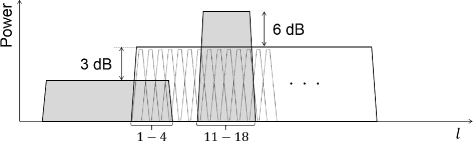
Interference scenario 1
Table 1 Simulation parameters -
Scenario 2: Three independent interferences. As shown in Fig. 6, interferences 1, 2, and 3 superpose on 4 (1 ≤ l ≤ 4, 11 ≤ l ≤ 14, and 21 ≤ l ≤ 24) subcarriers of desired signals, respectively. Each SIR is 3, 0, and −6 dB, respectively. That is,
$$w(t,l) \sim \left\{ \begin{array}{ll} CN(0, 0.50), & 1\leq l\leq 4, \\ CN(0, 1.00), & 11\leq l\leq 14, \\ CN(0, 3.98), & 21\leq l\leq 24, \\ 0, & \text{otherwise}. \end{array} \right. $$Fig. 6 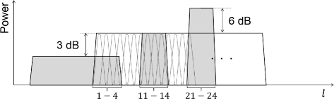
Interference scenario 2
-
Scenario 3: Three independent interferences. As shown in Fig. 7, interferences 1, 2, and 3 superpose on 4 (1≤l≤4, 11≤l≤14, and 21≤l≤24) subcarriers of desired signals, respectively. Each SIR is 3 dB, which corresponds to the assumption in the conventional schemes [15, 16]. That is,
$$w(t,l) \sim \left\{ \begin{array}{ll} CN(0, 0.50), & 1\leq l\leq 4, 11\leq l\leq 14, \\ & 21\leq l\leq 24, \\ 0, & \text{otherwise}. \end{array} \right. $$Fig. 7 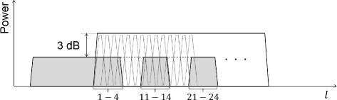
Interference scenario 3


Note that the interferences do not overlap each other in all scenarios. We evaluate detection rate and BER performance. In addition, we evaluate NRMSE of estimated interference power as a factor of the improvement.
In [15, 16], bit LLR is calculated in the same way as in Eq. (15), except that for all subcarriers, the same interference power is applied. On BER performance, five schemes including the proposed scheme are evaluated. The proposed scheme corresponds to “Proposed.” “Iteration,” “EM,” and “Averaging” correspond to conventional schemes [15–17], respectively. In “perfect,” the noise power, each interference power, and each superposed band are known to the receiver, where we can ideally calculate the bit LLR in Eq. (15).
5.1 Detection rate
Figures 8 and 9 show the detection rate of superposed bands for Averaging and Proposed under the interference scenarios 2 and 3, respectively. Detection rate is defined as a ratio of the number of packets where all interferences are correctly detected, to the number of transmitted packets. We show details of the legends in the following.
-
nItr: Number of times of iteration.
Fig. 8 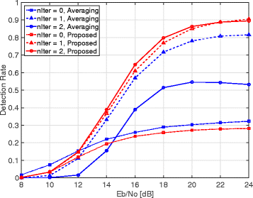
Detection rate for the scenario 2
Fig. 9 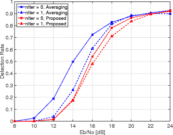
Detection rate for the scenario 3
-
Averaging: Moving average of three residual powers are taken in frequency domain. For every nItr, the interference detection is performed based on a threshold, which corresponds to Eq. (19). For nItr = 0, the threshold is set to the average of all residual powers in the packet. For nItr ≥ 1, the updated threshold is exploited. The threshold has been updated once for nItr = 1 and twice for nItr = 2.
-
Proposed: For nItr = 0, the interference detection is performed based on the threshold. That is, the decision is performed according to Eq. (19). The threshold is set to the average of all residual powers in the packet. For nItr ≥ 1, superposition probabilities are exploited to the decision, which corresponds to Eq. (22). Specifically, initially calculated superposition probabilities are used for nItr = 1 and updated ones for nItr = 2.


First, we discuss Fig. 8, where all interference power is different. For nItr = 0, the detection rate of Averaging is higher than that of Proposed. This improvement of Averaging is because of averaging residual powers in both time and frequency domains. As introduced in [17], the residual powers |r(t,l)|2 are averaged in time domain to mitigate the variance of residual powers among subcarriers superposed by the same interference. In addition, moving average of the obtained |r(l)|2 is taken in frequency domain for further mitigation of the variance. Therefore, with respect to the detection in Eq. (19), which is based on a threshold, the detection of Averaging is more accurate than that of Proposed. In contrast, the detection rate of Proposed exceeds that of Averaging for nItr ≥ 1. For example, the detection rate of Proposed is higher than that of Averaging by about 0.1 for nItr = 1 and E b /N 0 ≥ 20 dB. Besides, the detection rate of Averaging for nItr = 2 is greatly degraded from that for nItr = 1, while the detection rate of Proposed for nItr = 2 is improved from that for nItr = 1 except for E b /N 0 = 24 dB. In Averaging, the threshold is hard to be optimized when the difference of the interference power is large, because the equation for optimizing the threshold is derived on the assumption of equal interference power. Because the superposed band detection is performed with the inaccurate threshold, the detection rate gets degraded. In contrast, the superposition probabilities are substituted for the threshold to detect superposed bands for nItr ≥ 1 in Proposed. Superposed band detection with superposition probabilities is more reliable than that with threshold, because they are derived from the PDFs of residual powers for superposed and non-superposed bands. Exploiting the reliable indicator, the improved detection rate is obtained. Besides, the detection rate of Proposed is improved in comparison with that of Averaging in low E b /N 0 in the figure. For instance, the detection rate of Proposed is higher than that of Averaging by about 0.05 at E b /N 0 = 8 dB and by about 0.1 at E b /N 0 = 12 dB. In the case where the noise power is large and the interference power is small, it is difficult to detect the interference, because the interference signal is hidden in the noise signal. In contrast, in the case where the interference power is large like the interference scenario in Fig. 6, compared to the conventional scheme, the interference can be detected in the proposed scheme irrespective of the magnitude of the noise power. This is because the magnitude of the residual power on superposed bands is much larger than that on non-superposed bands.
Second, we discuss Fig. 9, where all interference power is equal. We omit the plots for nItr = 2, because the detection rate converges at nItr = 1. For both nItr = 0 and 1, the detection rate of Averaging outperforms that of Proposed, except for E b /N 0 = 24 dB. For example, for nItr = 0, the detection rate of Averaging is higher than that of Proposed by 0.3 at E b /N 0 = 14dB, and by 0.2 at E b /N 0 = 16 dB. As introduced for nItr = 0 in Fig. 8, this is because of the averaging of residual powers in both time and frequency domains. Similarly, for nItr = 1, Averaging is superior to Proposed. For example, the detection rate of Averaging is higher than that of Proposed by more than 0.1 at E b /N 0 = 16 dB and by 0.1 at E b /N 0 = 18 dB. This interference scenario is ideal for Averaging with respect to optimizing the threshold, because the equation for updating the threshold is derived based on the assumption of equal interference power. Thus, the threshold is calculated ideally, which leads to the high detection rate. On the other hand, although the superposition probabilities in Proposed are derived based on the PDFs of residual powers, it does not assure that the superposition probabilities are optimized. It may be possible to improve the detection rate of Proposed by modifying the derivation of the superposition probabilities, which is our future work.
5.2 BER performance
Figures 10, 11, and 12 show the BER performance under the scenarios 1, 2, and 3, respectively. The following are the settings in the simulations.
-
Iteration: Decoding is performed twice in total.
Fig. 10 
BER vs E b /N 0 for the scenario 1
Fig. 11 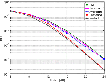
BER vs E b /N 0 for the scenario 2
Fig. 12 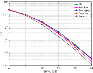
BER vs E b /N 0 for the scenario 3
-
Averaging: Moving average of three residual powers are taken. The threshold is updated twice, which corresponds to nItr = 2 in Section 5.1. Decoding is performed twice in total.
-
Proposed: The superposed probabilities are updated once, which corresponds to nItr = 2 in Section 5.1. Decoding is performed twice in total.


As shown in Fig. 10, Proposed achieves the better BER performance than that of other schemes for E b /N 0 ≥ 1 dB. Specifically, Proposed is improved compared to Iteration, EM, and Averaging by about 2 dB with respect to E b /N 0 for BER ≤ 10−3. This improvement is because of the following reasons. In Iteration and EM, one interference power is estimated by exploiting all residual powers on detected superposed bands. Thus, the schemes result in the worse BER performance when the difference of each interference power is large as in this scenario, because one estimated interference power cannot be accurate for all interferences. With regard to Averaging, though each interference power is estimated, it is hard to obtain accurate estimators. This is because the threshold is not optimized as in this scenario, which leads to the low detection rate. By contrast, Proposed can deal with both cases where each interference power is equal and different. This is because it detects each interference and estimates each power by using not the threshold but the superposition probabilities. Moreover, the BER performance of Proposed is very close to that of Perfect. This result is an evidence that accurate LLR is set in the proposed scheme.
Figure 11 shows the BER performance for the scenario 2. Similar to the result in Fig. 10, Proposed achieves the better BER performance than that of other schemes for E b /N 0 ≥ 12 dB. To be specific, for BER ≤ 10−4, Proposed is improved compared to others by more than 2 dB regarding E b /N 0. In the scenario 2, there exist three interferences with different power, which are more than the number of those in the scenario 1. Therefore, it is hard to detect the interferences accurately by using the one threshold.
In Fig. 12, all interference power is equal. The improvement of the BER performance by applying the proposed scheme is smaller than that in other scenarios, because this is the ideal scenario for the conventional schemes. However, Proposed shows the better BER performance than that of other schemes. Proposed tries to detect superposed bands iteratively based on not only the comparison of residual powers with a threshold but also superposition probabilities. Thus, we consider that each superposed band is correctly detected and each power is accurately estimated, which results in the better BER performance for the scenarios as well where each interference power is equal. Though the BER performance of Proposed is better than that of Averaging; however, as shown in Fig. 9, Averaging outperforms Proposed with respect to the detection rate. The reason why Proposed achieves the improvement of the BER performance compared to Averaging is the following. In Averaging, estimated interference power is never exploited to calculate LLR for non-superposed bands. Hence, even if the detection rate is high, LLR is sometimes set quite inaccurately when corresponding subcarrier is misdetected. By contrast, in Proposed, estimated interference power is applied to all subcarriers, irrespective of the result of the detection. Taking the possibility of misdetection into consideration, we weigh two PDFs with the superposition probabilities calculated based on the magnitude of residual powers. Therefore, we can avoid setting quite inaccurate LLR even when the misdetection happens. That is why, Proposed outperforms Averaging with respect to the BER performance.
5.3 NRMSE of estimated interference power
In this section, we evaluate NRMSE of the estimated interference power to confirm the relationship between the estimation accuracy of the interference power and the BER performance. Tables 2 and 3 show NRMSE of estimated interference power under the interference scenarios 2 and 3, respectively, where E b /N 0 ≥ 20 dB. In the tables, NRMSE is calculated as follows.
where N is the number of transmitted packets and \(\hat {\sigma }_{\text {if}}^{2}({l,j})\) is the estimated interference power for the packet j. On non-superposed bands, we cannot calculate the NRMSE because \(\sigma _{\text {if}}^{2}(l)~=~0\). Therefore, we show RMSE (root-mean-squared error) of the estimated interference power instead of NRMSE. The RMSE for non-superposed bands is calculated as follows.
In EM and Iteration, only one interference power \(\hat {\sigma }_{\text {if}}^{2}(j)\) is obtained. Thus, when NRMSE or RMSE is calculated for each subcarrier, \(\hat {\sigma }_{\text {if}}^{2}(j)\) is applied to all subcarriers on detected superposed bands. That is, for EM and Iteration,
where l and \(\overline {\mathbf {l}}\) are the set of indices of subcarriers on estimated superposed and non-superposed bands, respectively.
As shown in Table 2, NRMSE of Iteration is by far the largest among all the schemes with respect to the interferences 1 and 2. Thus, corresponding LLR is not set accurately, which results in the degradation of the BER performance. Regarding the interference 3, NRMSE of EM is the largest among all the schemes. In addition, SIR of the interference 3 is larger than that of any other interferences. Hence, the BER performance of EM is severely affected by the interference 3 due to inaccurate LLR. NRMSE of Averaging is almost the same as that of Proposed for interferences 2 and 3 and is smaller for the interference 1. However, the BER performance of Proposed is greatly improved from that of Averaging. This is due to the way of calculating LLR. In Averaging, each estimated interference power is not exploited to calculate LLR for estimated non-superposed bands. In other words, misdetection of superposed bands is not considered. In contrast, in Proposed, the misdetection is taken into account by weighting two PDFs with superposition probabilities. That is why, accurate LLR is obtained in Proposed, which results in the BER performance superior to that of Averaging.
In Table 3, all interference power is equal. With regard to each interference, NRMSE of schemes except for EM is almost the same. While the NRMSE of EM is the smallest among all the schemes, the RMSE is the largest. This should be the reason for the degradation of the BER performance. NRMSE of EM and Iteration is smaller than that of Averaging and Proposed, because the former assumes this interference scenario, where all interference power is equal. However, the BER performance of Proposed is improved compared to the conventional schemes. This is because of the way of deriving superposition probabilities and calculating LLR.
6 Conclusions
In this paper, we propose a scheme to suppress multiple wideband interferences based on superposition probabilities. In the proposed scheme, we derive the PDFs of residual powers for superposed and non-superposed bands. Based on residual powers and those PDFs, we calculate the superposition probability for each subcarrier. Furthermore, we perform superposed band detection iteratively according to the probability and update each estimated interference power. Through simulations, we showed that the detection rate of superposed bands is improved by iterating superposed band detection based on superposition probabilities. We also showed that the proposed scheme achieves the better BER performance than that of conventional ones.
References
A Goldsmith, Wireless communications (Cambridge University, Cambridge, 2005).
JM Peha, Approaches to spectrum sharing. Commun. Mag. IEEE. 43(2), 10–12 (2005). doi:10.1109/MCOM.2005.1391490.
T Sugiyama, H Kazama, M Morikura, S Kubota, S Kato, A frequency utilization efficiency improvement on superposed SSMAQPSK signal transmission over high speed QPSK signals in nonlinear channels. Commun. IEICE Trans.E76-B(5), 480–487 (1993).
J Mashino, T Sugiyama, in Personal, Indoor and Mobile Radio Communications, 2009 IEEE 20th International Symposium On. Total frequency utilization efficiency improvement by superposed multicarrier transmission scheme, (2009), pp. 1677–1681. doi:10.1109/PIMRC.2009.5450209.
D Qu, Z Wang, T Jiang, Extended active interference cancellation for sidelobe suppression in cognitive radio OFDM systems with cyclic prefix. IEEE Trans. Veh. Technol.59(4), 1689–1695 (2010). doi:10.1109/TVT.2010.2040848.
EHM Alian, P Mitran, in Global Communications Conference (GLOBECOM), 2012 IEEE. Improved active interference cancellation for sidelobe suppression in cognitive OFDM systems, (2012), pp. 1460–1465. doi:10.1109/GLOCOM.2012.6503319.
K Fazel, in Universal Personal Communications, 1994. Record., 1994 Third Annual International Conference On. Narrow-band interference rejection in orthogonal multi-carrier spread-spectrum communications, (1994), pp. 46–50. doi:s10.1109/ICUPC.1994.383042.
C Snow, L Lampe, R Schober, in Radio and Wireless Symposium, 2008 IEEE. Interference mitigation for coded MB-OFDM UWB, (2008), pp. 17–20. doi:10.1109/RWS.2008.4463417.
A Batra, JR Zeidler, in Acoustics, Speech and Signal Processing, 2009. ICASSP 2009. IEEE International Conference On. Narrowband interference mitigation in BICM OFDM systems, (2009), pp. 2605–2608. doi:10.1109/ICASSP.2009.4960156.
C Carlemalm, HV Poor, A Logothetis, Suppression of multiple narrowband interferers in a spread-spectrum communication system. Selected Areas Commun. IEEE J.18(8), 1365–1374 (2000). doi:10.1109/49.864002.
M Morelli, M Moretti, Improved decoding of BICM-OFDM transmissions plagued by narrowband interference. Wireless Commun. IEEE Trans.10(1), 20–26 (2011). doi:10.1109/TWC.2010.110510.091535.
L Sanguinetti, M Morelli, HV Poor, BICM decoding of jammed OFDM transmissions using the EM algorithm. Wireless Commun. IEEE Trans.10(9), 2800–2806 (2011). doi:10.1109/TWC.2011.062911.101448.
L Sanguinetti, M Morelli, G Imbarlina, An EM-based frequency offset estimator for OFDM systems with unknown interference. Wireless Commun. IEEE Trans.8(9), 4470–4475 (2009). doi:10.1109/TWC.2009.090063.
M Morelli, M Moretti, Channel estimation in OFDM systems with unknown interference. Wireless Commun. IEEE Trans.8(10), 5338–5347 (2009). doi:10.1109/TWC.2009.090270.
N Yoda, T Ohtsuki, J Mashino, T Sugiyama, Iterative decoding based on interference estimation in OFDM transmissions. IEICE Tech. Rep., RCS2014-3, 11–16 (2014).
N Yoda, T Ohtsuki, J Mashino, T Sugiyama, in Global Communications Conference (GLOBECOM), 2014 IEEE. Interference suppression using EM algorithm in ofdm transmissions, (2014), pp. 3249–3254. doi:10.1109/GLOCOM.2014.7037307.
Y Kakizaki, T Ohtsuki, J Mashino, in Personal, Indoor, and Mobile Radio Communications (PIMRC), 2015 IEEE 26th Annual International Symposium On. Suppression of multiple interferences for superposed multicarrier transmission, (2015), pp. 466–470. doi:10.1109/PIMRC.2015.7343344.
T Li, WH Mow, VKN Lau, M Siu, RS Cheng, RD Murch, Robust joint interference detection and decoding for OFDM-based cognitive radio systems with unknown interference. Selected Areas Commun. IEEE J.25(3), 566–575 (2007). doi:10.1109/JSAC.2007.070407.
S Kalyani, K Giridhar, in Communications, 2008. ICC ’08. IEEE International Conference On. Interference mitigation in turbo-coded OFDM systems using robust llrs, (2008), pp. 646–651. doi:10.1109/ICC.2008.127.
Competing interests
The authors declare that they have no competing interests.
Author information
Authors and Affiliations
Corresponding author
Rights and permissions
Open Access This article is distributed under the terms of the Creative Commons Attribution 4.0 International License(http://creativecommons.org/licenses/by/4.0/), which permits unrestricted use, distribution, and reproduction in any medium, provided you give appropriate credit to the original author(s) and the source, provide a link to the Creative Commons license, and indicate if changes were made.
About this article

Cite this article
Kakizaki, Y., Shibata, Y., Ohtsuki, T. et al. Suppression of multiple wideband interferences based on superposition probability. J Wireless Com Network 2016, 198 (2016). https://doi.org/10.1186/s13638-016-0699-9
Received:
Accepted:
Published:
DOI: https://doi.org/10.1186/s13638-016-0699-9