On the energy/spectral efficiency of multi-user full-duplex massive MIMO systems with power control

Abstract

In this paper, we consider a multi-user full-duplex (FD) massive multiple-input multiple-output (MIMO) system. The FD base station (BS) is equipped with large-scale antenna arrays, while each FD user is equipped with two antennas (one for transmission and the other one for reception). We assume that the channel state information (CSI) is imperfect, and no instantaneous CSI of loop interference (LI) channel is obtained. On the basis of low-complexity uplink beamforming and downlink precoding techniques, i.e. maximum-ratio combining/maximum-ratio transmission (MRC/MRT) and zero-forcing reception/zero-forcing transmission (ZFR/ZFT), the asymptotic expressions of signal-to-interference-plus-noise ratio (SINR) of uplink and downlink are derived respectively when the number of antennas of the BS tends to infinity. Based on the asymptotic SINR expressions, we first analyse the spectral efficiency (SE) performance assuming that the generalized power scaling scenario is adopted. Through the theoretical derivation, it is shown that the detrimental impact of the LI can be eliminated by the very large number of antennas at the BS if the power scaling scenario is appropriately applied, as well as the interference caused by the imperfect channel estimation, the multi-user interference (MUI) and inter-user interference (IUI). Then, we propose power allocation (PA) scenarios to maximize the energy efficiency (EE) and the sum SE with the constraint of maximum powers at the BS and users. The simulation results verify the accuracy of the asymptotic method, we also validate the effectiveness of the EE and the sum SE maximization PA algorithms. We show that adopting the PA scheme to maximize the sum SE can make the multi-user FD massive MIMO system outperform the half-duplex (HD) counterpart regardless of the level of LI.

1 Introduction

Now, the fourth generation (4G) wireless system has come to the mature stage, and with the booming development of all kinds of mobile smart terminals, the mobile Internet traffic in the recent years grows exponentially, which will increase by 1000 times beyond 2020. Meanwhile, the ratio of energy consumption in information technology system has been rapidly increasing, making it an urgent mission to decrease the energy consumption of the mobile communication systems. However, the current 4G is unable to satisfy the continuously increasing demands in the future mobile communication, which put forward a great challenge to the fifth generation (5G) wireless systems [1].

Adopting multiple-input multiple-output (MIMO) techniques is an essential way to utilize the wireless spatial resources and improve the spectral efficiency (SE) and energy efficiency (EE). Massive MIMO has been deemed to be one key technology for 5G, which uses large-scale antenna arrays (with orders of magnitude more antennas, e.g., 100 or more) to replace the currently adopted multiple antennas [2]. As the number of antennas grows larger, the simple linear precoder and detector tend to optimal, and the noise along with the uncorrelated interference can be ignored [3]. What is more, the spatial resolution of massive MIMO is remarkably enhanced compared with the conventional MIMO and can focus the signal beam within a narrow range; thus, the interference can be reduced by a wide margin [4], which as a result can significantly improve SE and EE [5].

On the parallel avenue, full duplex (FD) is another potential key technology for 5G. FD communication is the technology where signals are transmitted and received at the same time-frequency resource. In the conventional half-duplex (HD) systems, bi-direction link is separated by orthogonal time or frequency resources (the corresponding systems are time-division duplex (TDD) systems and frequency-division duplex (FDD) systems), where theoretically wastes half of the time-frequency resource. Nevertheless, in FD systems, due to the large amplitude difference between received signals and transmitted signals, signals leaking from the output to the input lead to severe loop interference (LI), typically 100 dB [6]. As a result, the primary task to apply FD technique is LI cancellation. With the development of signal processing techniques and hardware processing techniques, various kinds of LI cancellation techniques have been developed, including analog-domain LI cancellation [7], the cancellation of known signals in digital domain, or the combination of them [8, 9]. Because of the considerable potential of theoretically doubling the SE and making the usage of spectrum more flexible, FD technique has become a hotspot of research at present. For example, [10] analyses the complete achievable rate regions of a small-area radio system where a multiple-antennas FD access point serves two multiple-antennas HD devices, and the analytical results characterize the effect of self-interference at the access point and inter-device interference on the achievable rate regions. In [11], the authors consider the relay selection schemes for FD relaying protocol, over Nakagami-m fading channels, they show that the proposed schemes achieve better outage performance when compared with traditional schemes and are robust to the residual LI caused by the FD operation.

Those attractive benefits discussed above motivate researchers to combine massive MIMO and FD technique together so as to obtain better system performance. For example, FD massive MIMO relaying systems are considered in [12–14]. [12] considers a multi-pair FD decode-and-forward (DF) relay with maximum-ratio combining/maximum-ratio transmission (MRC/MRT) to process the signals, and the authors propose the use of massive antenna arrays at the relay station to significantly reduce the LI effect. In [13], a two-way FD relay system with FD users under MRC/MRT and zero-forcing reception/zero-forcing transmission (ZFR/ZFT) processing is considered, and four typical power scaling schemes are applied, then the upper bounds of the sum rates for each power scaling schemes are derived. It is shown that the LI can be decreased through reducing the power of FD relay. However, both [12] and [13] assume that some novel LI mitigation scenarios in [15] are applied, which is impractical in massive MIMO systems, and the reason will be explained in Section 2. [14] considers a multi-pair FD amplify-and-forward (AF) relaying system with ZFR/ZFT processing. It is shown that adopting low-complexity signal processing techniques can significantly decrease the detrimental impact of LI as well as multi-pair interference if the power scaling scheme is appropriately chosen, and FD systems combined with massive MIMO outperforms the HD counterpart in spectral efficiency even without active LI cancellation.

In this paper, we consider a multi-user FD massive MIMO system where the FD base station (BS) is equipped with large-scale antennas and each FD user is equipped with two antennas (one for transmitting and the other one for receiving) (Fig. 1). A general power scaling scenario is adopted at the BS or/and users to obtain a better EE performance. Note that the power scaling scenarios applied in [13, 16, 17] are just some special cases. It needs to be mentioned that this paper is different from [12] in several aspects: (a) a different approach is taken to derive the asymptotic expressions of uplink and downlink signal-to-interference-plus-noise ratio (SINR); (b) both the SE and EE are optimized; (c) new power scaling results on the SE and EE of multi-user FD massive MIMO system are obtained with the general power scaling scenario adopted at the BS and users. The main contributions of our work are as follows:

• A new asymptotic method is used to derive the asymptotic expressions of uplink and downlink SINR for the kth user, which turns out to be effective.

  Fig. 1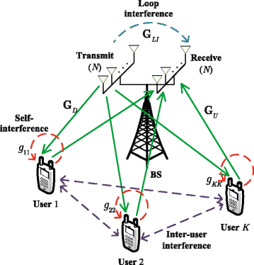

  

  Multi-user FD massive MIMO system with K users

• We adopt general power scaling scenario at the BS and users, and based on the derived SINR expressions, we analyse how the number of BS antennas and the transmit power of BS and users impact the system performance. To be specific, the transmit powers of users and BS are scaled down by 1/N ^p and 1/N ^q, respectively, where 0≤p,q≤1, and N represents the number of BS transmit or receive antennas. We show that as N grows larger, the harmful effect of LI can be wiped out when q>0 and the multi-user interference (MUI), CSI estimation error and inter-user interference (IUI) can be eliminated when p>0.

• We consider a power allocation (PA) scenario to control the transmit power at the BS and users so as to maximize the SE and EE, which is under the constraint of the maximum of transmit power.

Notation: We use boldface uppercase letter A and boldface lowercase letter a to represent matrix and column vector, respectively. ${\mathbb {E}}(\cdot)$, ∥·∥, (·)^∗, (·)^H, X(·), and Tr(·) stand for the expectation, the Euclidean norm, the conjugate, the conjugate transpose, the spectral radius of a matrix, and trace of a matrix, respectively. [A] _ij denotes the ith-row and jth-column entry of matrix A. I _N represents the N×N identity matrix. ${\mathcal {C}N} \left ({\mu,{\sigma ^{2}}}\right)$ stands for the complex-Gaussian distribution with mean of μ and variance of σ ². e _i represents a vector whose ith entry is 1 and the other are 0.

2 System model

We consider a multi-user FD massive MIMO system, where K users are within a single cell. Both the users and the BS operate in FD mode. We assume that the BS is equipped with two separate large-scale antennas arrays in which N for transmission and N for reception, while each user is equipped with two antennas in which one for transmitting signal and the other for receiving. All the users share the same time-frequency resource.

Let ${{\mathbf {G}}_{D}}=\,[{{\mathbf {\!g}}_{D,1}},\cdots,{{\mathbf {g}}_{D,K}}]\in {{\mathbb {C}}^{N\times K}}$ represent the downlink channel matrix between the transmit antenna array of the BS and the K users and let ${{\mathbf {G}}_{U}}=\,[{{\mathbf {\!g}}_{U,1}},\cdots,{{\mathbf {g}}_{U,K}}]\in {{\mathbb {C}}^{N\times K}}$ denote the uplink channel matrix between K users and the receive antenna array of the BS. G _a (a∈{D,U}) is modelled as ${{\mathbf {G}}_{a}}={{\mathbf {H}}_{a}}\mathbf {D}_{a}^{1/2}$, where ${{\mathbf {H}}_{a}}\in {{\mathbb {C}}^{N\times K}}$ characterizes the small-scale fading of the channel which has independent and identically distributed (i.i.d.) ${\mathcal {C}N}(0,1)$ elements, while D _a is the large-scale fading diagonal matrix whose kth diagonal entry [ D _a ] _kk =β _a,k denotes the large-scale fading coefficient. Moreover, ${{\mathbf {G}}_{\text {LI}}}=\,[\!{{\mathbf {g}}_{LI,1}},\cdots,{{\mathbf {g}}_{LI,N}}]\in {{\mathbb {C}}^{N\times N}}$ denotes the LI channel matrix between the transmit and receive antennas of the BS, whose entries are i.i.d. with distribution ${\mathcal {C}N}(0,{{\beta }_{\text {LI}}})$. ${{\mathbf {G}}_{IU}}=\,[{{\mathbf {\!g}}_{IU,1}},\cdots,{{\mathbf {g}}_{IU,K}}]\in {{\mathbb {C}}^{K\times K}}$ denotes the channel matrix between users whose entry [ G _IU ] _ij =g _ij represents the IUI channel coefficient from the ith user to the jth user, which are modelled as i.i.d. ${\mathcal {C}N}(0,{{\sigma }_{ij}})$. Note that [ G _IU ] _kk =g _kk denotes the coefficient of self-interference channel for the kth user.

2.1 Imperfect channel estimation phase

In [12] and [13], it made an assumption that the residual LI can be regarded as additive noise after applying some novel LI mitigation scenarios, on the basis of knowing the CSI of G _LI to compute the filter matrices [15]. It may work in the conventional MIMO systems where the antennas deployed at the relay or BS are in a small quantity. Nevertheless, with the growth of the number of transmit and receive antennas at the relay or BS, the dimension of G _LI increases, and in order to obtain the CSI of G _LI, the length of pilot sequence τ should satisfy τ≥N which is unprocurable in the massive MIMO systems owing to the limited duration of channel coherent time. Hence, in this paper, we assume that the instantaneous knowledge of G _LI is unknown and the CSI of G _U and G _D are obtained by MMSE estimation.

In order to realize the FD transmission, the informations of G _U and G _D need to be acquired at the BS¹. Therefore, during the channel coherent time, a part of the resource has to be assigned to the pilot sequences to do the channel estimation job. During the estimation phase, all the users’ antennas transmit the pilot sequences to the BS simultaneously². Then the received pilot signals at the transmit and receive antennas at the BS are written as

$$ {\mathbf{Y}_{R}} = \sqrt {\tau {P_{P}}} {\mathbf{G}_{RR}}{{\mathbf{X }}_{R}} + \sqrt {\tau {P_{P}}} {\mathbf{G}_{U}}{{\mathbf{X }}_{T}} + {\mathbf{N}_{R}}, $$

(1)

$$ {\mathbf{Y}_{T}} = \sqrt {\tau {P_{P}}} {\mathbf{G}_{D}}{{\mathbf{X }}_{R}} + \sqrt {\tau {P_{P}}} {\mathbf{G}_{TT}}{{\mathbf{X}}_{T}} + {\mathbf{N}_{T}}, $$

(2)

respectively, where τ is the length of the pilots, P _P denotes the transmit power of each pilot symbol; ${{\mathbf {G}}_{RR}}\in {{\mathbb {C}}^{N\times K}}$ and ${{\mathbf {G}}_{TT}}\in {{\mathbb {C}}^{N\times K}}$ denote the channels from the users’ transmit antennas to the transmit antennas of the BS and the users’ receive antennas to the receive antennas of the BS, respectively; ${{\mathbf {X }}_{R}}\in {{\mathbb {C}}^{K\times {\tau }}}$ and ${{\mathbf {X }}_{T}}\in {{\mathbb {C}}^{K\times {\tau }}}$ represent the pilot sequences which are transmitted from the receive antennas and transmit antennas of K users, respectively; N _R and N _T denote the AWGN matrices whose elements are i.i.d. ${\mathcal {C}N}(0,1)$. Note that all the pilot sequences are assumed to be orthogonal, i.e. ${{\mathbf {X }}_{a}}{{{\mathbf {X }}_{a}^{H}}} = {\mathbf{I}_{K}},a \in \left \{{R,T} \right \}$, and ${\mathbf {X }}_{R}{\mathbf {X }}_{T}^{H} = {{\mathbf {0}}_{K}}$.

Based on the MMSE estimation, the estimated channel matrices ${\hat {\mathbf {G}}_{U}}$ and ${\hat {\mathbf {G}}_{D}}$ can be expressed as

$$\begin{array}{*{20}l} {\hat{\mathbf{G}}_{U}} = \frac{1}{{\sqrt {\tau {P_{P}}} }}{\mathbf{Y}_{R}}{\mathbf{X }}_{T}^{H}{\boldsymbol{\Lambda}_{U}} = \left({\mathbf{G}_{U}} + \frac{1}{{\sqrt {\tau {P_{P}}} }}{{\tilde{\mathbf{N}}_{R}}} \right){\boldsymbol{\Lambda}_{U}}, \end{array} $$

(3)

$$\begin{array}{*{20}l} {\hat{\mathbf{G}}_{D}} = \frac{1}{{\sqrt {\tau {P_{P}}} }}{\mathbf{Y}_{T}}{\mathbf{X }}_{R}^{H}{\boldsymbol{\Lambda}_{D}} = \left({{\mathbf{G}_{D}} + \frac{1}{{\sqrt {\tau {P_{P}}} }}{{\tilde{\mathbf{N}}}_{T}}} \right){\boldsymbol{\Lambda}_{D}}, \end{array} $$

(4)

where ${\boldsymbol {\Lambda }_{U}} = {\left ({{\mathbf {D}_{U}^{- 1}} / {\left ({\tau {P_{P}}} \right)} + {\mathbf {I}_{K}}} \right)^{- 1}}$ and ${\boldsymbol {\Lambda }_{D}} = ({\mathbf {D}_{D}^{- 1}}/ {({\tau {P_{P}}})} + {\mathbf {I}_{K}})^{- 1}$ and ${\tilde {\mathbf {N}}_{R}} = {\mathbf {N}_{R}}{\mathbf {X}}_{T}^{H}$ and ${\tilde {\mathbf {N}}_{T}} = {\mathbf {N}_{T}}{\mathbf {X }}_{R}^{H}$, both of which have i.i.d. ${\mathcal {C}N}(0,1)$ elements due to the orthogonal rows of X _T and X _R .

According to the MMSE estimation, the channel matrices G _U and G _D can be decomposed as

$$\begin{array}{*{20}l} {\mathbf{G}_{i}} = {\hat{\mathbf{G}}_{i}} + \Delta {\mathbf{G}_{i}}, i \in \left\{ {U,D} \right\} \end{array} $$

(5)

where Δ G _i represents the estimation error matrix. According to the property of MMSE channel estimation, we can conclude that $\hat {\mathbf {G}}_{i}$ and Δ G _i are independent and the rows of them are mutually independent which comply with distributions ${\mathcal {C}N}(0, \hat {\mathbf {D}}_{i})$ and ${\mathcal {C}N}(0,\Delta \mathbf {D}_{i})$. Both $\hat {\mathbf {D}}_{i}$ and Δ D _i are diagonal matrices whose kth diagonal entries are expressed as ${{\hat \beta }_{i,k}} = {\tau {P_{P}}\beta _{i,k}^{2}} / \left ({\tau {P_{P}}{\beta _{i,k}} + 1} \right)$ and Δ β _i,k =β _i,k /(τ P _P β _i,k +1), respectively [5].

2.2 Data phase

The received signal at the BS can be expressed as

$$ {{\mathbf{y}}_{U}}=\sqrt{{{P}_{U}}}{{\mathbf{F}}^{H}}{{\mathbf{G}}_{U}}{{\mathbf{x}}_{U}}+\sqrt{{{P}_{D}}}{{\mathbf{F}}^{H}}{\mathbf{G}_{\text{LI}}} \mathbf{W}{{\mathbf{x}}_{D}}+{{\mathbf{F}}^{H}}{{\mathbf{n}}_{U}} $$

(6)

where $\mathbf {F}=\,[{{\mathbf {\!f}}_{1}},\cdots,{{\mathbf {f}}_{K}}]\in {{\mathbb {C}}^{N\times K}}$ denotes the uplink beamforming matrix; $\mathbf {W}=\,[{{\mathbf {w}}_{1}},\cdots,{{\mathbf {w}}_{K}}]\in {{\mathbb {C}}^{N\times K}}$ denotes the downlink precoding matrix; x _D =[ x _D,1,⋯,x _D,K ]^T and x _U =[ x _U,1,⋯,x _U,K ]^T represent the transmit signal vectors of the BS and users, respectively, with ${\mathbb {E}\{{\mathbf {x}_{a}}\mathbf {x}_{a}^{H}\}} = {\mathbf {I}_{K}}$, (a∈{D,U}); n _U ∼(0,σ _U I _N ) denotes the additive white Gaussian noise (AWGN) vector at the BS; and P _D and P _U denote the transmit powers of the BS and users, respectively.

The received signals at users, y _D , can be expressed as

$$\begin{array}{*{20}l} {{\mathbf{y}}_{D}}=\sqrt{{{P}_{D}}}\mathbf{G}_{D}^{H}\mathbf{W}{{\mathbf{x}}_{D}}+\sqrt{{{P}_{U}}}{{\mathbf{G}}_{IU}^{H}}{{\mathbf{x}}_{U}}+{{\mathbf{n}}_{D}} \end{array} $$

(7)

where n _D ∼(0,σ _D I _K ) denotes AWGN vector at users.

In order to keep the complexity low, the BS adopts linear processing techniques. With the linear beamforming and precoding matrices, the BS can separate the receive and transmit signals into K streams, i.e. y _U and y _D can be separated into K elements. The received signals of the kth user at the BS, i.e. the kth element of y _U is given by

$$ \begin{aligned} {{y}_{U,k}}=&\sqrt{{{P}_{U}}}\mathbf{f}_{k}^{H}{{\mathbf{g}}_{U,k}}{{x}_{U,k}}+\mathbf{f}_{k}^{H}{{\mathbf{n}}_{U}} \\ & +\underbrace{\sum\limits_{i=1,i\ne k}^{K}{\sqrt{{{P}_{U}}}}\mathbf{f}_{k}^{H}{{\mathbf{g}}_{U,i}}{{x}_{U,i}}}_{\text{MUI}}+\underbrace{\sqrt{{{P}_{D}}} \mathbf{f}_{k}^{H}{{\mathbf{G}}_{\text{LI}}}\mathbf{W}{{\mathbf{x}}_{D}}}_{\text{LI}}. \\ \end{aligned} $$

(8)

The first term of the right side of (8) is the transmit signal of the kth user. The second term is AWGN at the BS. The third term is the signals transmitted by users except the kth user, which is MUI for the kth user. The last term denotes LI at the BS. The received signal of the kth user can be expressed as

$$ \begin{aligned} {{y}_{D,k}}=&\sqrt{{{P}_{D}}}\mathbf{g}_{D,k}^{H}{{\mathbf{w}}_{k}}{{x}_{D,k}}+{{n}_{D,k}} \\ & +\underbrace{\sum\limits_{i=1,i\ne k}^{K}{\sqrt{{{P}_{D}}}}\mathbf{g}_{D,k}^{H}{{\mathbf{w}}_{i}}{{x}_{D,i}}}_{\text{MUI}}+ \underbrace{\sqrt{{{P}_{U}}}\mathbf{g}_{IU,k}^{H}{{\mathbf{x}}_{U}}}_{\text{IUI}}. \\ \end{aligned} $$

(9)

The first term of the right side of (9) is the downlink signal for the kth user. The second term is AWGN at the kth user. The third term is the MUI which is the downlink signal transmitted for other users. And the last term denotes the IUI comes from the signals transmitted by other users.

Before the analysis, we introduce the following lemma which is useful in the field of massive MIMO system.

Lemma 1

[[18], Lemma 1] Let A be a deterministic n×n complex matrix with uniformly bounded spectral radius for all n. Let $\mathbf {p}=\frac {1}{\sqrt {n}}{{\left [ {{p}_{1}},\cdots,{{p}_{n}} \right ]}^{T}}$ and $\mathbf {q}=\frac {1}{\sqrt {n}}{{\left [{{q}_{1}},\cdots {{q}_{n}} \right ]}^{T}}$ denote two mutually independent n×1 complex random vectors, whose elements are i.i.d. zero-mean random complex variables with unit variance and finite eighth moment. Then

$$ {{\mathbf{p}}^{H}}\mathbf{Ap}\to \frac{1}{n}\text{Tr}\left(\mathbf{A} \right)\text{and }{{\mathbf{p}}^{H}}\mathbf{Aq}\to 0 $$

(10)

almost surely as n→∞.

3 Analysis of asymptotic uplink and downlink SINR with MRC/MRT scenario

According to [19], with MMSE estimation at the BS, the uplink beamforming matrix F and downlink precoding matrix W based on the MRC/MRT scenario are given by

$$\begin{array}{*{20}l} & \mathbf{F}={\hat{\mathbf{G}}_{U}},\\\notag & \mathbf{W}={\hat{\mathbf{G}}_{D}}{{\left(\text{Tr}\left(\hat{\mathbf{G}}_{D}^{H}{\hat{\mathbf{G}}_{D}} \right) \right)}^{-1/2}}. \end{array} $$

(11)

3.1 Analysis of asymptotic uplink SINR

3.1.1 Asymptotic expression of uplink SINR

Substituting (5) and (11) into (8), the received signal for kth user at the BS can be re-expressed as

$$ \begin{aligned} \frac{{{y}_{U,k}}}{\sqrt{N}}= & \sqrt{N{{P}_{U}}}\frac{\hat{\mathbf{g}}_{U,k}^{H}{{\hat{\mathbf{g}}}_{U,k}}}{N}{{x}_{U,k}}+\frac{\hat{\mathbf{g}}_{U,k}^{H}{{\mathbf{n}}_{U}}}{\sqrt{N}} \\ & +I_{U,k}^{MUI}+I_{U,k}^{\Delta}+I_{U,k}^{\text{LI}} \\ \end{aligned} $$

(12)

where $I_{U,k}^{\text {MUI}}$, $I_{U,k}^{\Delta }$, and $I_{U,k}^{\text {LI}}$ denote the MUI, estimation error, and the LI, respectively, which can be expressed as

$$ \begin{aligned} & I_{U,k}^{\text{MUI}}=\sqrt{\frac{{{P}_{U}}}{N}}\sum\limits_{i=1,i\ne k}^{K}{\hat{\mathbf{g}}_{U,k}^{H}{{\hat{\mathbf{g}}}_{U,i}}{{x}_{U,i}}}, \\ & I_{U,k}^{\Delta}=\sqrt{\frac{{{P}_{U}}}{N}}\sum\limits_{i=1}^{K}{\hat{\mathbf{g}}_{U,k}^{H}{\Delta {\mathbf{g}}_{U,i}}{{x}_{U,i}}}, \\ & I_{U,k}^{\text{LI}}=\sqrt{\frac{{{P}_{D}}}{N}}\sum\limits_{i=1}^{K}{\frac{\hat{\mathbf{g}}_{U,k}^{H}{{\mathbf{G}}_{\text{LI}}}{{\hat{\mathbf{g}}}_{D,i}}}{\sqrt{\text{Tr(}\hat{\mathbf{G}}_{D}^{H}{\hat{\mathbf{G}}_{D}}\text{)}}}}{{x}_{D,i}}. \end{aligned} $$

(13)

According to Lemma 1 in [16] (i.e. the law of large number, LLN), the first two items of the right side of (12) can be obtained by

$$ \begin{aligned} & \frac{\hat{\mathbf{g}}_{U,k}^{H}{{\hat{\mathbf{g}}}_{U,k}}}{N}\xrightarrow[N\to \infty ]{a.s.}{\hat{{\beta }}_{U,k}}, \\ & \frac{\hat{\mathbf{g}}_{U,k}^{H}{{\mathbf{n}}_{U}}}{\sqrt{N}}\xrightarrow[N\to \infty ]{d}\mathsf{\mathcal{C}\mathcal{N}}(0,{{\hat \beta }_{U,k}}{{\sigma }_{U}}) \\ \end{aligned} $$

(14)

where $\xrightarrow [N\to \infty ]{a.s.}$ represents the almost sure convergence as N→∞ and $\xrightarrow [N\to \infty ]{d}$ denotes the convergence in distribution when N tends to infinity.

Then, the instantaneous power of MUI for the kth user at the BS can be given by

$$ \begin{aligned} & \mathbb{E}\mathrm{}\left[ {{{\left| {I_{U,k}^{\text{MUI}}} \right|}^{2}}} \right] = {P_{U}}N\sum\limits_{i = 1,i \ne k}^{K} {\frac{{\hat{\mathbf{g}}_{U,k}^{H}{\hat{\mathbf{g}}_{U,i}}\hat{\mathbf{g}}_{U,i}^{H}{\hat{\mathbf{g}}_{U,k}}}}{{{N^{2}}}}} \\ &= {P_{U}}N{{\hat \beta }_{U,k}}\sum\limits_{i = 1,i \ne k}^{K} {\frac{{{{\left\| {{{\hat{\mathbf{g}}}_{U,i}}} \right\|}^{2}}}}{N}\frac{{\hat{\mathbf{g}}_{U,k}^{H}}}{{\sqrt {N{{\hat \beta }_{U,k}}} }}} {\tilde{\mathbf{g}}_{U,i}}\tilde{\mathbf{g}}_{U,i}^{H}\frac{{{\hat{\mathbf{g}}_{U,k}}}}{{\sqrt {N{\hat \beta_{U,k}}} }} \end{aligned} $$

(15)

where the $\mathbb {E}\left [ \cdot \right ]$ operator is over x _U,k so as the following derivation, and ${\tilde {\mathbf {g}}_{U,i}}={{\hat {\mathbf {g}}}_{U,i}}/\left \| {{\hat {\mathbf {g}}}_{U,i}} \right \|$. Based on $X \left ({{\tilde {\mathbf {g}}_{u,i}}\tilde {\mathbf {g}}_{u,i}^{H}} \right) = {\text {Tr}}\left ({{\tilde {\mathbf {g}}_{u,i}}\tilde {\mathbf {g}}_{u,i}^{H}} \right) = {\mathrm {1}}$ and (10), we can obtain

$$ \frac{\hat{\mathbf{g}}_{U,k}^{H}}{\sqrt{N{{\hat \beta }_{U,k}}}}{\tilde{\mathbf{g}}_{U,i}}\tilde{\mathbf{g}}_{U,i}^{H}\frac{{{\hat{\mathbf{g}}}_{U,k}}}{\sqrt{N{{\hat \beta }_{U,k}}}}\xrightarrow[N\to \infty ]{a.s.}\frac{1}{N}. $$

(16)

According to (16) and LLN, the asymptotic expression of instantaneous power of MUI when the number of antennas at the BS approaches to infinity can be expressed as

$$ {\mathbb{E}}\mathrm{}\left[ {{\left| I_{U,k}^{\text{MUI}} \right|}^{2}} \right]\xrightarrow[N\to \infty ]{a.s.}{{P}_{U}}{{\hat \beta }_{U,k}}\sum\limits_{i=1,i\ne k}^{K}{{{\hat \beta }_{U,i}}}. $$

(17)

We can see from (13) that the expression of $I_{U,k}^{\Delta }$ is similar to that of $I_{U,k}^{\text {MUI}}$, and then, it is not difficult to utilize the same method to obtain ${\mathbb {E}} \left [ {{{\left | {I_{U,k}^{\Delta }} \right |}^{2}}} \right ]$ when N→∞ as

$$ {\mathbb{E}}\mathrm{}\left[ {{\left| I_{U,k}^{\Delta} \right|}^{2}} \right]\xrightarrow[N\to \infty ]{a.s.}{{P}_{U}}{{\hat{\beta }}_{U,k}}\sum\limits_{i=1}^{K}{\Delta }{{\beta }_{U,i}}. $$

(18)

Next, the power of $I_{U,k}^{\text {LI}}$ is given by

$$ \begin{aligned} & {\mathbb{E}}\mathrm{}\left[ {{\left| I_{U,k}^{\text{LI}} \right|}^{2}} \right]=\frac{{{P}_{D}}}{N}\sum\limits_{i=1}^{K}{\frac{\hat{\mathbf{g}}_{U,k}^{H}{{\mathbf{G}}_{\text{LI}}}{{\hat{\mathbf{g}}}_{D,i}}\hat{\mathbf{g}}_{D,i}^{H}\mathbf{G}_{\text{LI}}^{H}{{\hat{\mathbf{g}}}_{U,k}}}{\text{Tr(}\hat{\mathbf{G}}_{D}^{H}{\hat{\mathbf{G}}_{D}}\text{)}}} \\ & = {{P}_{D}}\sum\limits_{i=1}^{K}{\frac{{{\left\| {{\hat{\mathbf{g}}}_{D,i}} \right\|}^{2}}}{N}\frac{\hat{\mathbf{g}}_{U,k}^{H}{{\mathbf{G}}_{\text{LI}}}{{\tilde{\mathbf{g}}}_{D,i}}\tilde{\mathbf{g}}_{D,i}^{H}\mathbf{G}_{\text{LI}}^{H}{{\hat{\mathbf{g}}}_{U,k}}}{\text{Tr(}\hat{\mathbf{G}}_{D}^{H}{\hat{\mathbf{G}}_{D}}\text{)}}} \\ \end{aligned} $$

(19)

where ${\tilde {\mathbf {g}}_{D,i}}={{\hat {\mathbf {g}}}_{D,i}}/\left \| {{\hat {\mathbf {g}}}_{D,i}} \right \|$. Since $\text {rank}\left ({{\tilde {\mathbf {g}}}_{D,i}}{{\tilde {\mathbf {g}}}^{H}}_{D,i} \right)=\text {Tr} \left ({{\tilde {\mathbf {g}}}_{D,i}}{{\tilde {\mathbf {g}}}^{H}}_{D,i} \right)=1$, we can get ${\tilde {\mathbf {g}}_{D,i}}{\tilde {\mathbf {g}}^{H}}_{D,i} = \mathbf {U}{\text {diag}}\left ({{\mathbf {e}_{1}}} \right){\mathbf {U}^{H}}$, where U is a unitary matrix. We define G ^′ _LI=G _LI U, then (19) is equivalently expressed as

$${} \begin{aligned} &{\mathbb{E}}\left[ {{\left| I_{U,k}^{\text{LI}} \right|}^{2}} \right]=\\ &{{P}_{D}}\sum\limits_{i=1}^{K}{\frac{{{\left\| {{\hat{\mathbf{g}}}_{D,i}} \right\|}^{2}}}{N}}\frac{\hat{\mathbf{g}}_{U,k}^{H}{{{\mathbf{{G'}}}}_{\text{LI}}}\text{diag}\left({{\mathbf{e}}_{1}} \right)\mathbf{{G'}}_{\text{LI}}^{H}{{\hat{\mathbf{g}}}_{U,k}}}{\text{Tr}\left(\hat{\mathbf{G}}_{D}^{H}{\hat{\mathbf{G}}_{D}} \right)} \\ &={{P}_{D}}N\frac{{{\hat \beta }_{U,k}}}{\text{Tr}\left(\frac{\hat{\mathbf{G}}_{D}^{H}{\hat{\mathbf{G}}_{D}}}{N} \right)} \\ &\quad\times\sum\limits_{i=1}^{K}{\frac{{{\left\| {{\hat{\mathbf{g}}}_{D,i}} \right\|}^{2}}}{N}\frac{{{\left\| {{{\mathbf{{g}'}}}_{LI,1}} \right\|}^{2}}}{N}\frac{\hat{\mathbf{g}}_{U,k}^{H}}{\sqrt{N{{\hat \beta }_{U,k}}}}{{{\tilde{\mathbf{g}}'}}}_{LI,1}}{{\tilde{\mathbf{g'}}}^{H}}_{LI,1}\frac{{{\hat{\mathbf{g}}}_{U,k}}}{\sqrt{N{{\hat \beta }_{U,k}}}} \\ \end{aligned} $$

(20)

where g ^′ _{L I,1}=g ^′ _{L I,1}/∥g ^′ _{L I,1}∥, and the latter equality of (20) is derived by the manipulation of ${{\mathbf {{G}'}}_{\text {LI}}}\text {diag}({{\mathbf {e}}_{1}})\mathbf {{G}'}_{\text {LI}}^{H}={{\mathbf {{g}'}}_{LI,1}}{{\mathbf {{g'}}}_{LI,1}^{H}}={{\left \| {{{\mathbf {{g}'}}}_{LI,1}} \right \|}^{2}}{{\tilde {\mathbf {g}}'}}_{LI,1}{\tilde {\mathbf {g'}}^{H}}_{LI,1}$. Based on the property that $X \left ({{\tilde {\mathbf {g'}}_{b,1}}\tilde {\mathbf {g'}}_{LI,1}^{H}} \right) = {\text {Tr}}\left ({{\tilde {\mathbf {g'}}_{LI,1}}\tilde {\mathbf {g'}}_{LI,1}^{H}} \right) = {\mathrm {1}}$ and Lemma 1, it can be derived that

$$ \frac{\hat{\mathbf{g}}_{U,k}^{H}}{\sqrt{N{{\hat \beta }_{U,k}}}}{{\tilde{\mathbf{g}}'}}_{LI,1}\tilde{\mathbf{g'}}_{LI,1}^{H}\frac{{{\hat{\mathbf{g}}}_{U,k}}}{\sqrt{N{{\hat \beta }_{U,k}}}}\xrightarrow[N\to \infty ]{a.s.}\frac{1}{N}, $$

(21)

and based on LLN, we have

$$ \frac{\mathbf{G}_{D}^{H}{{\mathbf{G}}_{D}}}{N}\xrightarrow[N\to \infty ]{a.s.}{{\mathbf{D}}_{D}}. $$

(22)

Substituting (21) and (22) into (20), then the power of LI as N approaches to infinity is written as

$$ {\mathbb{E}}\mathrm{}\left[ {{\left| I_{U,k}^{\text{LI}} \right|}^{2}} \right]\xrightarrow[N\to \infty ]{a.s.} {{P}_{D}}{{\hat \beta }_{U,k}}{{\beta }_{\text{LI}}}. $$

(23)

As a result, substituting (14), (17), (18), and (23) into (10), we can get the asymptotic uplink SINR for the kth user under MRC/MRT scheme as

$$ \gamma_{U,k}^{MR} = \frac{{N{P_{U}}{\hat \beta_{U,k}}}}{{{P_{U}}\sum\limits_{i = 1,i \ne k}^{K} {{\hat \beta_{U,i}} + {P_{U}}\sum\limits_{i = 1}^{K} {\Delta {\beta_{U,i}}} + {P_{D}}{\beta_{\text{LI}}}} + {\sigma_{U}}}}. $$

(24)

3.1.2 Uplink power scaling analysis

When the number of BS antennas grows larger, we can scale down P _U or/and P _D by the number of antennas while maintaining the desired performance. Hence, we consider the generalized scaling scenarios P _U =E _U /N ^p and P _D =E _D /N ^q, substituting which into (24) we can obtain the power-scaled asymptotic uplink SINR as

$$\begin{array}{*{20}l} \tilde \gamma_{U,k}^{MR} = \frac{{{N^{1 - p}}{E_{U}}{{\hat \beta }_{U,k}}}}{{\frac{{{E_{U}}}}{{{N^{p}}}}\sum\limits_{i = 1,i \ne k}^{K} {{{\hat \beta }_{U,i}}} + \frac{{{E_{U}}}}{{{N^{p}}}}\sum\limits_{i = 1}^{K} {\Delta {\beta_{U,i}}} + \frac{{{E_{D}}}}{{{N^{q}}}}{\beta_{\text{LI}}} + {\sigma_{U}}}} \end{array} $$

(25)

where 0≤p,q≤1. We consider four typical power scaling scenarios in this part.

• Case 1, p=q=0: We assume there is no power scaling at the BS and users. It is obvious that under case 1, the uplink SINR tends to infinity as N→∞ when there is no power scaling scheme adopted. From (25), we can see that all components (including the MUI, channel estimation error (CEE), LI, and the noise at the BS) which have baneful impact on the kth user diminish when N→∞, while the desired signal is maintained. The reason is that in the regime of large N, the MUI is averaged. Similarly, due to the sufficient diversity gain and power constraint of the BS, the rest of the unexpected signals at the BS approach to zero when N tends to infinity.

• Case 2, 0<p≤1,q=0: Case 2 is the power scaling scheme only adopted at the users. When 0<p<1, all the detrimental signals are averaged out as N→∞, which is similar to case 1. However, when the power of users are scaled down by N, i.e. p=1, although the harmful effect of MUI and CEE are eliminated as N grows larger, the LI and the noise at the BS cannot be wiped out, which makes the uplink SINR tends to a ceiling value as N→∞.

• Case 3, p=0,0<q≤1: Case 3 denotes the power scaling scheme adopted at the BS. From Eq. (25), it can be seen that the asymptotic SINR of case 3 becomes infinite when N→∞, which is similar to case 1. What is more, the ${\frac {1}{N}}$ factor before LI indicates that, with power scaling at the BS, the harmful effect of LI which is amplified by the BS can be diminished when N approaches to infinity.

• Case 4, 0<p≤1,0<q≤1: Case 4 represents the power scaling scenario applied both at the BS and users. When q=1, it can be observed from (25) that the detrimental effect of MUI, CEE, and LI disappear as N→∞ while the noise at the BS cannot be eliminated, under which situation the noise at the BS poses greater influence to the uplink SE performance when N is large. When 0<q<1, all the unexpected signals vanish when N approaches to infinity.

3.2 Analysis of asymptotic downlink SINR

3.2.1 Asymptotic expression of downlink SINR

Substituting (5) and (11) into (9), the received signal of the kth user can be rewritten as

$$ \begin{aligned} {{y}_{D,k}}=& \sqrt{N{{P}_{D}}}\frac{\hat{\mathbf{g}}_{D,k}^{H}{{\hat{\mathbf{g}}}_{D,k}}}{\sqrt{N}\sqrt{\text{Tr} (\hat{\mathbf{G}}_{D}^{H}\hat{\mathbf{G}}_{D})}}{{x}_{D,k}}+{{n}_{D,k}} \\ & +I_{D,k}^{\text{MUI}}+I_{D,k}^{\Delta}+I_{D,k}^{IUI} \\ \end{aligned} $$

(26)

where $I_{U,k}^{\text {IUI}}$ represents the IUI, which along with $I_{U,k}^{\text {MUI}}$ and $I_{U,k}^{\Delta }$ can be expressed as

$$ \begin{aligned} & I_{D,k}^{\text{MUI}}=\sum\limits_{i=1,i\ne k}^{K}{\sqrt{{{P}_{D}}}}\frac { \mathbf{g}_{D,k}^{H}{{\hat{\mathbf{g}}}_{D,i}}}{\sqrt{\text{Tr}\left(\hat{\mathbf{G}}_{D}^{H}{\hat{\mathbf{G}}_{D}} \right)}}{{x}_{D,i}}, \\ & I_{D,k}^{\Delta}=\sum\limits_{i=1}^{K}{\sqrt{{{P}_{D}}}}\frac{\Delta \mathbf{g}_{D,k}^{H}{{\hat{\mathbf{g}}}_{D,i}}}{\sqrt{\text{Tr}\left(\hat{\mathbf{G}}_{D}^{H}{\hat{\mathbf{G}}_{D}} \right)}}{{x}_{D,i}}, \\ & I_{D,k}^{\text{IUI}}=\sum\limits_{i=1}^{K}{\sqrt{{{P}_{U}}}{{g}_{ik}^{*}}{{x}_{U,i}}}. \end{aligned} $$

(27)

According to LLN, the first item of the right side of (26) can be expressed as

$$ \begin{aligned} \frac{\hat{\mathbf{g}}_{D,k}^{H}{{\hat{\mathbf{g}}}_{D,k}}}{\sqrt{N}\sqrt{\text{Tr}(\hat{\mathbf{G}}_{D}^{H}{\hat{\mathbf{G}}_{D}})}}&={{\left(\text{Tr}\left(\frac{\hat{\mathbf{G}}_{D}^{H}{\hat{\mathbf{G}}_{D}}}{N} \right) \right)}^{-1/2}}\frac{\hat{\mathbf{g}}_{D,k}^{H}{{\hat{\mathbf{g}}}_{D,k}}}{N} \\ & \xrightarrow[N\to \infty ]{a.s.}{{\hat \beta }_{D,k}}{{\left(\text{Tr}\left({{\hat{\mathbf{D}}}_{D}} \right) \right)}^{-1/2}}. \end{aligned} $$

(28)

Similar with the derivation of (17) and (18), the instantaneous power of $I_{Dk}^{\text {MUI}}$ and I Dk Δ when N tends to infinity for the kth downlink user are expressed as

$$ {\mathbb{E}}\left[ {{\left| I_{D,k}^{\text{MUI}} \right|}^{2}} \right]\xrightarrow[N\to \infty ]{a.s.}\frac{1}{\text{Tr}\left({{{\hat{\mathbf{D}}}}_{D}} \right)}{{P}_{D}}{{\hat{\beta }}_{D,k}}\sum\limits_{i=1,i\ne k}^{K}{{{\hat \beta }_{D,i}}}, $$

(29)

$$ {\mathbb{E}}\mathrm{}\left[ {{\left| I_{D,k}^{\Delta} \right|}^{2}} \right]\xrightarrow[N\to \infty ]{a.s.}\frac{1}{\text{Tr}\left({{{\hat{\mathbf{D}}}}_{D}} \right)}{{P}_{D}}\Delta {{\beta }_{D,k}}\sum\limits_{i=1}^{K}{{{{\hat{\beta }}}_{D,i}}}. $$

(30)

It is easy to achieve the instantaneous power of the interference introduced by IUI as

$$ {\mathbb{E}}\left[ {{{\left| {I_{D,k}^{\text{IUI}}} \right|}^{2}}} \right] = {P_{U}}\sum\limits_{i = 1}^{K} {{\sigma_{ik}}}. $$

(31)

Then, substituting (28), (29), (30), and (31) into (26), the asymptotic downlink SINR for the kth user with MRC/MRT processing can be achieved as (32), shown below.

$$ \begin{aligned} \gamma_{D,k}^{MR} = \frac{{N{P_{D}}\hat \beta_{D,k}^{2}}}{{{P_{D}}{{\hat \beta }_{D,k}}\sum\limits_{i = 1,i \ne k}^{K} {{\hat \beta_{D,i}}} + {P_{D}}\Delta {\beta_{D,k}}\sum\limits_{i = 1}^{K} {{\hat \beta_{D,i}}} + {\text{Tr}}\left({{\hat {\mathbf{D}}_{D}}} \right){P_{U}}\sum\limits_{i = 1}^{K} {{\sigma_{ik}}} + {\text{Tr}}\left({{\hat {\mathbf{D}}_{D}}} \right){\sigma_{D}}}} \end{aligned} $$

(32)

$$ \begin{aligned} \tilde \gamma_{D,k}^{MR} \,=\, \frac{{{N^{1 - q}}{E_{D}}\hat \beta_{D,k}^{2}}}{{\frac{{{E_{D}}}}{{{N^{q}}}}{{\hat \beta }_{D,k}}\sum\limits_{i = 1,i \ne k}^{K} {{\hat \beta_{D,i}}} + \frac{{{E_{D}}}}{{{N^{q}}}}\Delta {\beta_{D,k}}\sum\limits_{i = 1}^{K} {{\hat \beta_{D,i}}} {\mathrm{+ Tr}}\left({{\hat{\mathbf{D}}_{D}}} \right)\frac{{{E_{U}}}}{{{N^{p}}}}\sum\limits_{i = 1}^{K} {{\sigma_{ik}}} \,+\, {\text{Tr}}\left({{\hat{\mathbf{D}}_{D}}} \right){\sigma_{D}}}} \end{aligned} $$

(33)

3.2.2 Downlink power scaling analysis

The power-scaled asymptotic downlink SINR is given by (33), shown above. Similarly, we analyse the impact of scaling power on the downlink SINR

• Case 1, p=q=0: (33) implies that the downlink SINR of case 1 tends to infinity when N→∞. All the MUI, CEE, IUI, and the noise at the kth user are wiped out as N goes to infinity, and only the desired signal is maintained.

• Case 2, 0<p≤1,q=0: From (33), we can see that the downlink SINR of case 2 goes to infinity when N is large enough. Different from case 1, we can conclude that scaling down the transmit power of users can decrease the detrimental effect of IUI which is amplified by it.

• Case 3, p=0,0<q≤1: In case 3, MUI and CEE are eliminated when N is large enough. Nevertheless, when q=1, due to the remained baneful effect of IUI and AWGN at the kth user, the asymptotic downlink SINR for case 3 tends to be deterministic when N approaches infinity. If 0<q<1, the SINR increases without upper bound as N grows.

• Case 4, 0<p≤1,0<q≤1: When N→∞, MUI, CEE, and IUI tend to be eliminated. Similar to uplink case 4, when q=1, the detrimental effect of noise at kth user still remains, the AWGN at the users has more influence to the downlink SE for large N. When 0<q<1, all the harmful signals disappear and the downlink SINR tends to infinity when N grows infinite.

Remark: From the above analysis, we can conclude that scaling down the BS power can decrease the adverse effect of LI and cutting down the user power can minish the MUI, CEE, and IUI. However, decrease P _U and P _D can also decrease the SE, which as a result exits a tradeoff between EE and SE, and we will discuss it in the simulation section.

4 Analysis of asymptotic uplink and downlink SINR with ZFR/ZFT processing

According to [19], the beamforming and precoding matrices based on the ZFR/ZFT scenario are given by

$$ \begin{aligned} &\mathbf{F} = {\hat{\mathbf{G}}_{U}}{\left({\hat{\mathbf{G}}_{U}^{H}{\hat{\mathbf{G}}_{U}}} \right)^{- 1}},\\ &\mathbf{W} = {\hat{\mathbf{G}}_{D}}{\left({\hat{\mathbf{G}}_{D}^{H}{\hat{\mathbf{G}}_{D}}} \right)^{- 1}}{\left({{\text{Tr}}\left({{{\left({\hat{\mathbf{G}}_{D}^{H}{\hat{\mathbf{G}}_{D}}} \right)}^{- 1}}} \right)} \right)^{- 1/2}}. \end{aligned} $$

(34)

4.1 Analysis of asymptotic uplink SINR

Substituting (34) into (8), the received signal for kth user at the BS can be rewritten as

$$\begin{array}{*{20}l} \sqrt N {y_{U,k}} =& \sqrt {N{P_{U}}} {x_{U,k}} + \sqrt N \mathbf{e}_{k}^{T}{\left({\hat{\mathbf{G}}_{U}^{H}{\hat{\mathbf{G}}_{U}}} \right)^{- 1}}\hat{\mathbf{G}}_{U}^{H}{\mathbf{n}_{U}}\\ \notag &+ I_{U,k}^{\Delta} + I_{U,k}^{\text{LI}} \end{array} $$

(35)

where $I_{U,k}^{\Delta }$ and $I_{U,k}^{\text {LI}}$ are expressed as

$$ \begin{aligned} I_{U,k}^{\Delta} =& \sqrt {N {P_{U}}} \mathbf{e}_{k}^{T}{\left({\hat{\mathbf{G}}_{U}^{H}{\hat{\mathbf{G}}_{U}}} \right)^{- 1}}\hat{\mathbf{G}}_{U}^{H}\sum\limits_{i = 1}^{K} {\Delta {\mathbf{g}_{U,i}}{x_{U,i}}}, \\ I_{U,k}^{\text{LI}} =& \sqrt {N {P_{U}}} \mathbf{e}_{k}^{T}{\left({\hat{\mathbf{G}}_{U}^{H}{\hat{\mathbf{G}}_{U}}} \right)^{- 1}}\hat{\mathbf{G}}_{U}^{H}{\mathbf{G}_{\text{LI}}} \\ &\times\frac{{{\hat{\mathbf{G}}_{D}}{{\left({\hat{\mathbf{G}}_{D}^{H}{\hat{\mathbf{G}}_{D}}} \right)}^{- 1}}}}{{\sqrt {{\text{Tr}}\left({{{\left({\hat{\mathbf{G}}_{D}^{H}{\hat{\mathbf{G}}_{D}}} \right)}^{- 1}}} \right)} }}{\mathbf{x}_{D}}. \end{aligned} $$

(36)

According to LLN, the asymptotic expression of the second term of the right side of (35) can be derived as

$$ \begin{aligned} \sqrt{N}\mathbf{e}_{k}^{T}{{\left(\hat{\mathbf{G}}_{U}^{H}{\hat{\mathbf{G}}_{U}} \right)}^{-1}}\hat{\mathbf{G}}_{U}^{H}{{\mathbf{n}}_{U}}=&\mathbf{e}_{k}^{T}{{\left(\frac{\hat{\mathbf{G}}_{U}^{H}{\hat{\mathbf{G}}_{U}}}{N} \right)}^{-1}}\frac{\hat{\mathbf{G}}_{U}^{H}{{\mathbf{n}}_{U}}}{\sqrt{N}} \\ & \xrightarrow[N\to \infty ]{a.s.}\hat{\beta }_{U,k}^{-1}{{{\tilde{n}}}_{U.k}} \\ \end{aligned} $$

(37)

where ${\tilde n_{U,k}}$ obeys ${\mathcal {C}N}(0,{{{\hat \beta }_{U,k}}{\sigma _{U}}})$.

From (36), ${\mathbb {E}}\left [ {{{\left | {I_{D,k}^{\Delta }} \right |}^{2}}} \right ]$ can be represented as

$$ \begin{aligned} {\mathbb{E}}\left[ {{\left| I_{U,k}^{\Delta} \right|}^{2}} \right]&=\frac{1}{N}{{P}_{D}}\sum\limits_{i=1}^{K}{\mathbf{e}_{k}^{T}{{\left(\frac{\hat{\mathbf{G}}_{U}^{H}{\hat{\mathbf{G}}_{U}}}{N} \right)}^{-1}}} \\ &\quad\times \hat{\mathbf{G}}_{U}^{H}\Delta {{\mathbf{g}}_{U,i}}\Delta \mathbf{g}_{U,i}^{H}{\hat{\mathbf{G}}_{U}}{{\left(\frac{\hat{\mathbf{G}}_{U}^{H}{\hat{\mathbf{G}}_{U}}}{N} \right)}^{-1}}{{\mathbf{e}}_{k}} \\ &=N{{P}_{D}}\hat{\beta }_{U,k}^{-2}\sum\limits_{i=1}^{K}{\frac{\hat{\mathbf{g}}_{U,k}^{H}\Delta {{\mathbf{g}}_{U,i}}\Delta \mathbf{g}_{U,i}^{H}{{\hat{\mathbf{g}}}_{U,k}}}{{{N}^{2}}}} \\ \end{aligned} $$

(38)

where the latter equality is according to LLN. Then, the approximate expression of ${\mathbb {E}}\left [ {{{\left | {I_{D,k}^{\Delta }} \right |}^{2}}} \right ]$ can be derived in the method adopted in (15), which can be obtained as

$$ \begin{aligned} {\mathbb{E}}\left[ {{{\left| {I_{D,k}^{\Delta}} \right|}^{2}}} \right]\xrightarrow[N\to \infty ]{a.s.}{{P}_{D}}\hat \beta_{U,k}^{-1}\sum\limits_{i=1}^{K}{\Delta {{\beta }_{U,i}}} \end{aligned} $$

(39)

Next, the power of ${I_{U,k}^{\text {LI}}}$ can be written from (36) as

$$ \begin{aligned} &{\mathbb{E}}\left[ {{{\left| {I_{U,k}^{\text{LI}}} \right|}^{2}}} \right] = \\ &\frac{1}{{{N^{2}}}}\frac{{{P_{D}}}}{{{\text{Tr}}\left({{{\left({\frac{{\hat{\mathbf{G}}_{D}^{H}{\hat{\mathbf{G}}_{D}}}}{N}} \right)}^{- 1}}} \right)}}\mathbf{e}_{k}^{T}{\left({\frac{{\hat{\mathbf{G}}_{U}^{H}{\hat{\mathbf{G}}_{U}}}}{N}} \right)^{- 1}}\hat{\mathbf{G}}_{U}^{H}{\mathbf{G}_{\text{LI}}}\\ & \times {\hat{\mathbf{G}}_{D}}{\left({\frac{{\hat{\mathbf{G}}_{D}^{H}{\hat{\mathbf{G}}_{D}}}}{N}} \right)^{- 2}}\hat{\mathbf{G}}_{D}^{H}\mathbf{G}_{\text{LI}}^{H}{\hat{\mathbf{G}}_{U}}{\left({\frac{{\hat{\mathbf{G}}_{U}^{H}{\hat{\mathbf{G}}_{U}}}}{N}} \right)^{- 1}}{\mathbf{e}_{k}}. \end{aligned} $$

(40)

Then, based on LLN, we can obtain the asymptotic expression of (40) as

$$ \begin{aligned} {\mathbb{E}} \left[ {{\left| I_{U,k}^{\text{LI}} \right|}^{2}} \right]\xrightarrow[N\to \infty ]{a.s.}&\frac{{{P}_{D}}}{{{N}^{2}}}\frac{1}{\text{Tr}\left(\hat{\mathbf{D}}_{U}^{-1} \right)}\mathbf{e}_{k}^{T}\hat{\mathbf{D}}_{U}^{-1}\hat{\mathbf{G}}_{U}^{H}{{\mathbf{G}}_{\text{LI}}}{\hat{\mathbf{G}}_{D}} \\ &\times \hat{\mathbf{D}}_{D}^{-2}\hat{\mathbf{G}}_{D}^{H}\mathbf{G}_{\text{LI}}^{H}{\hat{\mathbf{G}}_{U}}\hat{\mathbf{D}}_{U}^{-1}{{\mathbf{e}}_{k}} \\ =\frac{{{P}_{D}}}{{{N}^{2}}}&\frac{1}{\text{Tr}\left(\hat{\mathbf{D}}_{U}^{-1} \right)}\hat{\beta }_{U,k}^{-2}\sum\limits_{i=1}^{K}{\hat \beta_{D,i}^{-2}{{\left\| {{\hat{\mathbf{g}}}_{D,i}} \right\|}^{2}}} \\ & \times \hat{\mathbf{g}}_{U,k}^{H}{{\mathbf{G}}_{\text{LI}}}{{{\hat{\mathbf{g}}}}_{D,i}}\hat{\mathbf{g}}_{D,i}^{H}\mathbf{G}_{\text{LI}}^{H}{{\hat{\mathbf{g}}}_{U,k}}. \end{aligned} $$

(41)

We can observe that (41) has the similar form as (19), then using the similar approach of (19), i.e. ${\hat {\mathbf {g}}_{D,i}}{{\hat {\mathbf {g}}}^{H}}_{D,i} = {\left \| {{\hat {\mathbf {g}}_{D,i}}} \right \|^{2}}\mathbf {U}{\text {diag}}\left ({{\mathbf {e}_{1}}} \right){\mathbf {U}^{H}}$, (41) can be derived as

$$ \begin{aligned} {\mathbb{E}}\left[ {{\left| I_{U,k}^{\text{LI}} \right|}^{2}} \right]&= N{{P}_{D}}\frac{1}{\text{Tr}\left(\hat{\mathbf{D}}_{U}^{-1} \right)}\hat{\beta }_{U,k}^{-1}\sum\limits_{i=1}^{K}{\hat \beta_{D,i}^{-2}\frac{{{\left\| {{{\hat{\mathbf{g}}}}_{D,i}} \right\|}^{2}}}{N}} \\ & \quad \times \frac{{{\left\| {{{\mathbf{{g}'}}}_{LI,1}} \right\|}^{2}}}{N}\frac{\hat{\mathbf{g}}_{U,k}^{H}}{\sqrt{N{{{\hat{\beta }}}_{U,k}}}}{{\tilde{\mathbf{g}'}}_{LI,1}}\tilde{\mathbf{g'}}_{LI,1}^{H}\frac{{{\hat{\mathbf{g}}}_{U,k}}}{\sqrt{N{{\hat \beta }_{U,k}}}} \\ & \quad\xrightarrow[N\to \infty ]{a.s.}{{P}_{D}}\hat{\beta }_{U,k}^{-1}{{\beta }_{\text{LI}}}. \end{aligned} $$

(42)

In the end, by substituting (37), (39), and (42) into (35), we can obtain the asymptotic uplink SINR with ZFR/ZFT processing as

$$ \gamma_{U,k}^{ZF} = \frac{{N{P_{U}}{{\hat \beta }_{U,k}}}}{{{P_{U}}\sum\limits_{i = 1}^{K} {\Delta {\beta_{U,i}}} + {P_{D}}{\beta_{\text{LI}}} + {\sigma_{U}}}}. $$

(43)

Since the method of derivation and analysis for the power-scaled ZFR/ZFT scheme is similar to the MRC/MRT cases, therefore, we omit them.

4.2 Analysis of asymptotic downlink SINR

Substituting (34) into (9), the received signal of kth user can be expressed as

$$ \begin{aligned} {y_{D,k}} = &\sqrt {N{P_{D}}} \frac{1}{{\sqrt {{\text{Tr}}\left({{{\left({\frac{{\hat{\mathbf{G}}_{D}^{H}{\hat{\mathbf{G}}_{D}}}}{N}} \right)}^{- 1}}} \right)} }}{x_{D,k}} + {n_{D,k}}\\ &+ I_{D,k}^{\Delta} + I_{D,k}^{\text{IUI}} \end{aligned} $$

(44)

where $I_{D,k}^{\Delta }$ and $I_{D,k}^{\text {IUI}}$ are written as

$$\begin{array}{*{20}l} &I_{D,k}^{\Delta} = \sqrt {N{P_{D}}} \frac{{\Delta \mathbf{g}_{D,k}^{H}{\hat{\mathbf{G}}_{D}}{{\left({\hat{\mathbf{G}}_{D}^{H}{\hat{\mathbf{G}}_{D}}} \right)}^{- 1}}}}{{\sqrt {{\text{Tr}}\left({{{\left({\frac{{\hat{\mathbf{G}}_{D}^{H}{\hat{\mathbf{G}}_{D}}}}{N}} \right)}^{- 1}}} \right)} }}{\mathbf{x}_{D}},\\ \notag &I_{D,k}^{\text{IUI}}=\sum\limits_{i=1}^{K}{\sqrt{{{P}_{U}}}{{g}_{ik}^{*}}{{x}_{U,i}}}. \end{array} $$

(45)

Based on LLN, we have

$$ \frac{\hat{\mathbf{G}}_{D}^{H}{\hat{\mathbf{G}}_{D}}}{N}\xrightarrow[N\to \infty ]{a.s.}{{\hat{\mathbf{D}}}_{D}}. $$

(46)

According to (46), the asymptotic expression of the power of ${I_{D,k}^{\Delta } }$ in (45) is achieved by

$$ \begin{aligned} &{\mathbb{E}}\left[ {{\left| I_{D,k}^{\Delta} \right|}^{2}} \right]\xrightarrow[N\to \infty ]{a.s}\\ &\frac{N{{P}_{D}}}{\text{Tr}\left(\hat{\mathbf{D}}_{D}^{-1} \right)}\frac{\Delta \hat{\mathbf{g}}_{D,k}^{H}{{{\hat{\mathbf{G}}}}_{D}}\hat{\mathbf{D}}_{D}^{-2}\hat{\mathbf{G}}_{D}^{H}\Delta \hat{\mathbf{g}}_{D,k}^{H}}{{{N}^{2}}}. \end{aligned} $$

(47)

Based on Lemma 1, we can achieve

$$ \begin{aligned} {\mathbb{E}}\left[ {{\left| I_{D,k}^{\Delta} \right|}^{2}} \right]=&\frac{N{{P}_{D}}}{\text{Tr}\left(\hat{\mathbf{D}}_{D}^{-1} \right)}\Delta {{\beta }_{D,k}}\sum\limits_{i=1}^{K}{\hat{\beta }_{D,i}^{-2}} \\ & \times \frac{{{\left\| {{{\hat{\mathbf{g}}}}_{D,i}} \right\|}^{2}}}{N}\frac{\Delta \mathbf{g}_{D,k}^{H}}{\sqrt{N{{{\hat{\beta }}}_{D,k}}}}{{\tilde{\mathbf{g}}}_{D,i}}\tilde{\mathbf{g}}_{D,i}^{H}\frac{\Delta {{\mathbf{g}}_{D,k}}}{\sqrt{N{{\hat \beta }_{D,k}}}} \\ \xrightarrow[N\to \infty ]{a.s.}&{{P}_{D}}\Delta {{\beta }_{D,k}}. \end{aligned} $$

(48)

Hence, according to (48) and (31), the asymptotic downlink SINR of the kth user under ZFR/ZFT scenario is achieved as

$$\begin{array}{*{20}l} \gamma_{D,k}^{ZF} = \frac{{N{P_{D}}}}{{{\text{Tr}}\left({\hat{\mathbf{D}}_{D}^{- 1}} \right)\left({{P_{D}}\Delta {\beta_{D,k}} + {P_{U}}\sum\limits_{i = 1}^{K} {{\sigma_{ik}}} + {\sigma_{D}}} \right)}}. \end{array} $$

(49)

Remark: Based on the above analysis, we define the uplink asymptotic SE C _U , downlink asymptotic SE C _D , and sum asymptotic SE C _sum as

$$ \begin{aligned} &{C_{U}} = \frac{{T - \tau }}{T}\sum\limits_{k = 1}^{K} {{{\log }_{2}}(1 + {\gamma_{U,k}})}, \\ &{C_{D}} = \frac{{T - \tau }}{T}\sum\limits_{k = 1}^{K} {{{\log }_{2}}(1 + {\gamma_{D,k}})}, \\ &{C_{\text{sum}}} = {C_{U}} + {C_{D}}, \end{aligned} $$

(50)

respectively. In order to validate the accuracy of the asymptotic method in this paper, we compare our asymptotic SE with the ergodic SE. In Section 6, Monte-Carlo simulation method is adopted to generate the ergodic SE curve in the figures of the simulation results, and we will show that the approximate results are quiet tight even when N is small (e.g., N=25).

5 Power control

Obviously, the primary intention of applying FD techniques in wireless communication systems is to enhance the SE performance. It is worth noting that since the uplink and downlink channels transmit simultaneously and LI cancellation techniques are adopted in FD systems; therefore, more energy is consumed than the HD counterpart. Due to the increasing attention to green communications, EE is another metric widely used in many systems to evaluate the performance, especially in massive MIMO systems where enhancing the EE performance is significant [5].

Observing (24), (32), (43), and (49), we can see that the SINR of each user is different due to the different fading channels each user experiences, and in the previous sections, the transmit powers of K users, i.e. P _U , are all assumed to be the same, and the powers allocated to the K streams of downlink signals are fixed, which as a result may not achieve the optimal SE/EE performance. Hence, in this section, we assume the transmit power of kth user and the power allocated to the kth downlink stream are different and propose the PA schemes to maximize the sum SE and EE subject to power constraints, which are called SE PA and EE PA for short.

5.1 Maximization of the SE

In this section, we assume that the transmit power of kth user and the power allocated to the kth downlink stream are P _U,k and P _D,k ∥w _k ∥², respectively. Then, we can formulate the SE optimization problem as

$$ \begin{aligned} &\mathop {{\text{max}}}\limits_{{\cal {P}}} \;\;{C_{\text{sum}}}\\ &{\text{s.t. }}\left\{ {\begin{array}{l} p_{1}:0 \le {P_{U,k}} \le {{P}_{U}},k = 1, \cdots,K,\\ p_{2}:{\sum\limits_{k = 1}^{K} {{P_{D,k}}{{\left\| {{\mathbf{w}_{k}}} \right\|}^{2}}} \le {{P}_{D}}},\\ p_{3}:{P_{D,k}} \ge 0,k = 1, \cdots,K \end{array}} \right. \end{aligned} $$

(51)

where ={P _U,1,⋯,P _U,K ,P _D,1,⋯,P _D,K } and C _sum is defined in (50).

In order to facilitate the analysis, we first rewrite the asymptotic uplink and downlink SINR as

$$\begin{array}{*{20}l} {\gamma_{U,k}} = \frac{{{P_{U,k}}{A_{k}}}}{{\sum\limits_{i = 1}^{K} {{P_{U,i}}{B_{k,i}}} + \sum\limits_{i = 1}^{K} {{P_{D,i}}} C_{i} + 1}}, \end{array} $$

(52)

$$\begin{array}{*{20}l} {\gamma_{D,k}} = \frac{{{P_{D,k}}{D_{k}}}}{{\sum\limits_{i = 1}^{K} {{P_{D,i}}{E_{k,i}}} + \sum\limits_{i = 1}^{K} {{P_{U,i}}} {F_{k,i}} + 1}} \end{array} $$

(53)

which represent the unified uplink and downlink SINR expressions of MRC/MRT and ZFR/ZFT, respectively. For more details, with MRC/MRT scheme, we have

$$ \begin{aligned} &{A_{k}} = {{N{{\hat \beta }_{U,k}}} / {{\sigma_{U}}}},\\ &{B_{k,i}} = \left\{ \begin{array}{l} {{\Delta {\beta_{U,i}}} / {{\sigma_{U}}},i = k}\\ {{{\left({{{\hat \beta }_{U,i}} + \Delta {\beta_{U,i}}} \right)} / {{\sigma_{U}}}},i \ne k} \end{array} \right.,\\ &C_{i} = {{{{\left\| {{\mathbf{w}_{i}}} \right\|}^{2}}{\beta_{\text{LI}}}} / {{\sigma_{U}}}},\\ &D_{k} = {{N\hat \beta_{D,k}^{2}} / {{\text{Tr}}\left({{\hat{\mathbf{D}}_{D}}} \right){\sigma_{D}}}},\\ &{E_{k,i}} = \left\{ {\begin{array}{l} {{{\Delta {\beta_{D,k}}{{\hat \beta }_{D,i}}} / {\left({{\text{Tr}}\left({{{\hat{\mathbf{D}}}_{D}}} \right){\sigma_{D}}} \right)}},i = k}\\ {\frac{{{{\hat \beta }_{D,k}}{{\hat \beta }_{D,i}} + \Delta {\beta_{D,k}}{{\hat \beta }_{D,i}}}}{{{\text{Tr}}\left({{{\hat{\mathbf{D}}}_{D}}} \right){\sigma_{D}}}},i \ne k} \end{array}} \right.,\\ &{F_{k,i}} = {{{\sigma_{ik}}} / {{\sigma_{D}}}}. \end{aligned} $$

(54)

For ZFR/ZFT processing scheme, we have

$$ \begin{aligned} &{A_{k}} = {{N{{\hat \beta }_{U,k}}} / {{\sigma_{U}}}},\\ &{B_{k,i}} = {{\Delta {\beta_{U,i}}} / {{\sigma_{U}}}},\\ &C_{i} = {{{{\left\| {{\mathbf{w}_{i}}} \right\|}^{2}}{\beta_{\text{LI}}}} / {{\sigma_{U}}}},\\ &D_{k} = {{N} / {\left({{\text{Tr}}\left({\hat{\mathbf{D}}_{D}^{- 1}} \right){\sigma_{D}}} \right)}}\\ &{E_{k,i}} = {{{{\left\| {{\mathbf{w}_{i}}} \right\|}^{2}}\Delta {\beta_{D,k}}} / {{\sigma_{D}}}},\\ &{F_{k,i}} = {{{\sigma_{ik}}} / {{\sigma_{D}}}}. \end{aligned} $$

(55)

Based on (50), (51), (52), and (53), we can rewrite the SE optimization problem as

$$ \begin{aligned} &\mathop {{\text{max}}}\limits_{{\cal {P}}} {\text{ }}\prod\limits_{k = 1}^{K} {\left[ {\left({1 + {\gamma_{U,k}}} \right)\left({1 + {\gamma_{D,k}}} \right)} \right]} \\ &=\mathop {\text{min}}\limits_{{\cal {P}}}\;\;\prod\limits_{k = 1}^{K} {{{\left[ {\left({1 + {\gamma_{U,k}}} \right)\left({1 + {\gamma_{D,k}}} \right)} \right]}^{- 1}}} \\ &{\text{s.t. }}\left\{ {\begin{array}{l} c_{1}:{{\gamma_{U,k}} \le \frac{{{P_{U,k}}{A_{k}}}}{{\sum\limits_{i = 1}^{K} {{P_{U,i}}{B_{k,i}}} + \sum\limits_{i = 1}^{K} {{P_{D,i}}} C_{i} + 1}}},\\ \qquad k = 1, \cdots, K\\ c_{2}:{{\gamma_{D,k}} \le \frac{{{P_{D,k}}D}}{{\sum\limits_{i = 1}^{K} {{P_{D,i}}{E_{k,i}}} + \sum\limits_{i = 1}^{K} {{P_{U,i}}} {F_{k,i}} + 1}}},\\ \qquad k = 1, \cdots, K\\ p_{1},p_{2},p_{3} \end{array}} \right. \end{aligned} $$

(56)

where p ₁, p ₂, and p ₃ are power constraints given by (51).

We can see that the form of SE optimization problem in (56) is very close to a geometric programming (GP) except for the target which is not in the posynomial form [20]. Fortunately, we can use the technique in [21] to approximate the target so as to use convex optimization tools to solve (56). To be specific, 1+γ _a,k can be approximated by ${\lambda _{a,k}}\gamma _{a,k}^{{\mu _{a,k}}}$ close to a point ${{\hat \gamma }_{a,k}}$, where ${\mu _{a,k}} = {{\hat \gamma }_{a,k}}{\left ({1 + {{\hat \gamma }_{a,k}}} \right)^{- 1}}$, ${\lambda _{a,k}} = \hat \gamma _{a,k}^{- {\mu _{a,k}}}\left ({1 + {{\hat \gamma }_{a,k}}} \right)$, and a∈{U,D}. Thus, (56) can be reformulated as (57), shown below.

$$ \begin{aligned} &\mathop {{\text{min}}}\limits_{\mathcal{P}}\!\! {\text{ }}\prod\limits_{k = 1}^{K} {{{\left({{\lambda_{U,k}}{\lambda_{D,k}}} \right)}^{- 1}}\gamma_{U,k}^{- {\mu_{U,k}}}\gamma_{D,k}^{- {\mu_{D,k}}}} \\ &{\text{s.t. }}\!\!\!\left\{ {\begin{array}{l} \!\!\!c_{1}:\!\!\! {\frac{1}{{{A_{k}}}}\!\!\sum\limits_{i = 1}^{K}\!\! {{B_{k,i}}P_{U,k}^{- 1}{P_{U,i}}} {\gamma_{U,k}} \!\,+\,\! \frac{1}{{{A_{k}}}}\!\!\sum\limits_{i\! =\! 1}^{K} \!\!{C_{i}P_{U,k}^{- 1}{P_{D,i}}} {\gamma_{U,k}} \!\,+\,\! A_{k}^{\,-\, 1}P_{U,k}^{\,-\, 1}{\gamma_{U,k}} \!\le\!\! 1,k \,=\, 1,\! \cdots\!, K},\\\!\!\! c_{2}\!\!:\!\! {\frac{1}{D_{k}}\!\!\sum\limits_{i = 1}^{K}\!\! {{E_{k,i}}{P_{D,i}}P_{D,k}^{- 1}{\gamma_{D,k}}} \!\,+\,\! \frac{1}{D_{k}}\!\!\!\sum\limits_{i = 1}^{K} {{F_{k,i}}\!{P_{U,i}}} P_{D,k}^{- 1}{\gamma_{D,k}} \!\!\,+\,\! {D_{k}^{\,-\, 1}}P_{D,k}^{- 1}{\gamma_{D,k}} \!\!\le\!\! 1,k \,=\, 1, \cdots\!, K},\\ {{p}_{1}},{{p}_{2}},{{p}_{3}} \end{array}} \right. \end{aligned} $$

(57)

In this way, the SE optimization problem in (57) becomes a standard GP which can be solved by the Algorithm 1.

5.2 Maximization of the EE

The EE is defined as

$$\begin{array}{*{20}l} {\eta_{\text{EE}}} = \frac{{{C_{\text{sum}}}}}{{\sum\limits_{k = 1}^{K} {\left({{P_{U,k}} + {P_{D,k}}} \right)} + {P_{\text{cir}}}}},k = 1, \cdots,K. \end{array} $$

(58)

where P _cir is the power consumed by the circuits.

Then we can formulate the EE optimization problem as

$$ \begin{aligned} &\mathop {{\text{max}}}\limits_{{\cal {P}}} {\text{ }}{\eta_{\text{EE}}}\\ &{\text{s.t. }}\left\{ {\begin{array}{l} {{C_{\text{sum}}} \ge {{\bar C}_{\text{sum}}}},\\ p_{1},p_{2},p_{3} \end{array}} \right. \end{aligned} $$

(59)

where ${{\bar C}_{\text {sum}}}$ denotes the required sum SE.

For the sake of illustration, define

$$\begin{array}{*{20}l} {\mathcal{C}} = \left\{ {{\cal {P}}\left| \begin{array}{l} 0 \le {P_{U,k}} \le {{P}_{U}},{P_{D,k}} \ge 0,\\ {\sum\limits_{i = 1}^{K} {{P_{D,i}}{{\left\| {{\mathbf{w}_{i}}} \right\|}^{2}}} \le {P_{D}}},\\ k = 1, \cdots, K \end{array} \right.} \right\}, \end{array} $$

(60)

$$\begin{array}{*{20}l} {P_{\text{sum}}} = \sum\limits_{k = 1}^{K} {\left({{P_{U,k}} + {P_{D,k}}} \right)} + P_{\text{cir}} \end{array} $$

(61)

According to [22], solving the EE-maximization problem, we can introduce the following three auxiliary subproblems

$$ \begin{aligned} & \left({{\mathrm{Q}}_{1}} \right)\ {\cal {P}}_{{{\mathrm{Q}}_{1}} }^{*}=\arg \ \underset{{\cal {P}}\in {\mathcal{C}}}{\mathop{\max }}\,\ {{C}_{\text{sum}}}, \\ & \left({{\mathrm{Q}}_{2}} \right)\ {\cal {P}}_{{{\mathrm{Q}}_{2}} }^{*}=\arg \ \underset{{\cal {P}}\in {\mathcal{C}}}{\mathop{\max }}\,\ \frac{{{C}_{\text{sum}}}}{{{P}_{\text{sum}}}}, \\ & \left({{\mathrm{Q}}_{3}} \right)\ {\cal {P}}_{{{\mathrm{Q}}_{3}} }^{*}=\arg \ \underset{{\cal {P}}\in {\mathcal{C}},{{C}_{\text{sum}}}={{\bar C}_{\text{sum}}}}{\mathop{\min }}\,\ {{P}_{\text{sum}}}. \\ \end{aligned} $$

(62)

Solving the EE maximization problem (59) can be separated into three steps: (a) Check whether the optimal solution of problem Q₁, i.e., Q₁∗ satisfies the SE constraint. If it does, go to (b). If not, then the problem is infeasible. (b) Check whether the optimal solution of problem Q₂ satisfies the SE constraint. If it satisfies, then Q₂∗ is the solution of (59). Otherwise, go to (c), i.e. obtain Q₃∗ of problem Q₃ which is the solution of (59). In this paper, the required sum SE ${{\bar C}_{\text {sum}}}$ and the power constraints are set to make the EE maximization problem feasible. Next, the detailed solutions to the subproblems Q₂ and Q₃ are introduced in the following subsections.

5.2.1 Solution to problem Q₂

Observing the function of sum SE we can see that C _sum can be rewritten as

$$\begin{array}{*{20}l} {C_{\text{sum}}} = n\left({\cal {P}} \right) - d\left({\cal {P}} \right) \end{array} $$

(63)

where

$$ \begin{aligned} &n\left({\cal {P}} \right)\\ & = \sum\limits_{k = 1}^{K} {{{\log }_{2}}} \left({\sum\limits_{i = 1}^{K} {{P_{U,i}}{B_{k,i}}} + \sum\limits_{i = 1}^{K} {{P_{D,i}}C_{i}} + 1 + {P_{U,k}}{A_{k}}} \right)\\ & \quad\,+\, \sum\limits_{k = 1}^{K} {{{\log }_{2}}\left({\sum\limits_{i = 1}^{K} {{P_{D,i}}{E_{k,i}}} \,+\, \sum\limits_{i = 1}^{K} {{P_{U,i}}} {F_{k,i}} \,+\, 1 \,+\, {P_{D,k}}D_{k}} \right)}, \end{aligned} $$

(64)

$$ \begin{aligned} &\quad d\left({\cal {P}} \right)\\ & = \sum\limits_{k = 1}^{K} {{{\log }_{2}}} \left({\sum\limits_{i = 1}^{K} {{P_{U,i}}{B_{k,i}}} + \sum\limits_{i = 1}^{K} {{P_{D,i}}C_{i}} + 1} \right)\\ & \quad+ \sum\limits_{k = 1}^{K} {{{\log }_{2}}\left({\sum\limits_{i = 1}^{K} {{P_{D,i}}{E_{k,i}}} + \sum\limits_{i = 1}^{K} {{P_{U,i}}} {F_{k,i}} + 1} \right)} \end{aligned} $$

(65)

which is generally non-convex due to the convexity of (64) and (65). In order to make (63) convex, we use the convexity to linearly approximate d(), i.e., based on log(1+x)≤ log(1+x ₀)+(1+x ₀)⁻¹(x−x ₀) for x≥0, the upper bound of d() at the nth iteration is given by

$$ \begin{aligned} &{{\bar d}^{\left(n \right)}}\left({\cal {P}} \right)\\ & = \sum\limits_{k = 1}^{K} {\left[ {{{\log }_{2}}\left({1 + z_{U,k}^{\left({n - 1} \right)}} \right) + \frac{{{z_{U,k}} - z_{U,k}^{\left({n - 1} \right)}}}{{1 + z_{U,k}^{\left({n - 1} \right)}}}} \right]} \\ & \quad+ \sum\limits_{k = 1}^{K} {\left[ {{{\log }_{2}}\left({1 + z_{D,k}^{\left({n - 1} \right)}} \right) + \frac{{{z_{D,k}} - z_{D,k}^{\left({n - 1} \right)}}}{{1 + z_{D,k}^{\left({n - 1} \right)}}}} \right]} \end{aligned} $$

(66)

where ${z_{U,k}} = \sum \limits _{i = 1}^{K} {{P_{U,i}}{B_{k,i}}} + \sum \limits _{i = 1}^{K} {{P_{D,i}}C_{i}}$, $z_{U,k}^{\left ({n - 1} \right)} = \sum \limits _{i = 1}^{K} {P_{U,i}^{\left ({n - 1} \right)}{B_{k,i}}} + \sum \limits _{i = 1}^{K} {P_{D,i}^{\left ({n - 1} \right)}C_{i}}$, ${z_{D,k}} = \sum \limits _{i = 1}^{K} {{P_{D,i}}{E_{k,i}}} + \sum \limits _{i = 1}^{K} {{P_{U,i}}} {F_{k,i}}$, and $z_{D,k}^{\left ({n - 1} \right)} = \sum \limits _{i = 1}^{K} {P_{D,i}^{\left ({n - 1} \right)}{E_{k,i}}} + \sum \limits _{i = 1}^{K} {P_{U,i}^{\left ({n - 1} \right)}} {F_{k,i}}$. Here, ${\{ P_{U,i}^{\left ({n - 1} \right)}\} }$ and ${\{ P_{D,i}^{\left ({n - 1} \right)}\} }$ denote the value of {P _U,i } and {P _D,i } at the (n−1)th iteration.

Therefore, the EE maximization problem at the nth iteration can be formulated as

$$ \begin{aligned} & \underset{{\cal {P}}}{\mathop{\text{max}}}\,\ \frac{n\left({\cal {P}} \right)-{{{\bar{d}}}^{\left(n \right)}}\left({\cal {P}} \right)}{{{P}_{\text{sum}}}} \\ & \text{s.t.} \quad {{p}_{1}},{{p}_{2}},{{p}_{3}} \\ \end{aligned} $$

(67)

Based on the fraction form, we can use the Dinkelbach-type algorithm [23], i.e. by introducing a parameter λ to solve the convex optimization problem for λ≤λ ^optimal

$$ \begin{aligned} & \underset{{\cal {P}}}{\mathop{\text{max}}}\,\ n\left({\cal {P}} \right)-{{{\bar{d}}}^{\left(n \right)}}\left({\cal {P}} \right)-\lambda {{P}_{\text{sum}}} \\ & \text{s.t.} \quad {{p}_{1}},{{p}_{2}},{{p}_{3}} \\ \end{aligned} $$

(68)

In conclusion, the method to solving the subproblem Q₂ is given in detail by Algorithm 2.

5.2.2 Solution to problem Q₃

We can reformulate the Q₃ problem as

$$ \begin{aligned} &\underset{\mathcal{P}}{\mathop{\text{min}}}\,\text{ }{{P}_{\text{sum}}}\\ &{\text{s.t. }}\left\{ {\begin{array}{l} c_{1}:\frac{T - \tau}{T}\sum\limits_{k = 1}^{K} {{{\log }_{2}}\left[ {\left({1 \,+\, {\gamma_{U,k}}} \right)\left({1 \,+\, {\gamma_{D,k}}} \right)} \right]} = {C_{\text{sum}}},\\ c_{2}:{{\gamma_{U,k}} \le \frac{{{P_{U,k}}{A_{k}}}}{{\sum\limits_{i = 1}^{K} {{P_{U,i}}{B_{k,i}}} + \sum\limits_{i = 1}^{K} {{P_{D,i}}} C_{i} + 1}}}\\ \qquad k = 1, \cdots, K,\\ c_{3}:{{\gamma_{D,k}} \le \frac{{{P_{D,k}}D_{k}}}{{\sum\limits_{i = 1}^{K} {{P_{D,i}}{E_{k,i}}} + \sum\limits_{i = 1}^{K} {{P_{U,i}}} {F_{k,i}} + 1}}}\\ \qquad k = 1, \cdots, K,\\ p_{1},p_{2},p_{3} \end{array}} \right. \end{aligned} $$

(69)

It can be observed that we can use the similar asymptotic method of (57), then EE maximization problem can be reformulated as (70), shown below. Since the algorithm solving (70) is similar to Algorithm 1, only the objective function and constraints are different; therefore, we omit the algorithm of solving problem Q₃ due to the page limitation.

$$ {{} {\begin{aligned} & \underset{\mathcal{P}}{\mathop{\text{min}}}\,\text{ }{{P}_{\text{sum}}} \\ & \text{s.t.} \left\{ \begin{array}{ll} c_{1}&: \prod\limits_{k=1}^{K}{\left(1+{{\gamma }_{Uk}} \right)\left(1+{{\gamma }_{Dk}} \right)}={{2}^{\frac{T{{{\bar{C}}}_{\text{sum}}}}{T-\tau}}}, \\ c&: \frac{1}{{{A_{k}}}}\sum\limits_{i = 1}^{K} {{B_{k,i}}P_{U,k}^{- 1}{P_{U,i}}} {\gamma_{U,k}} + \frac{1}{{{A_{k}}}}\sum\limits_{i = 1}^{K} {C_{i}P_{U,k}^{- 1}{P_{D,i}}} {\gamma_{U,k}} \\&+ A_{k}^{- 1}P_{U,k}^{- 1}{\gamma_{U,k}} \le 1,k = 1, \cdots, K, \\ c_{3}&: \frac{1}{D_{k}}\sum\limits_{i = 1}^{K} {{E_{k,i}}{P_{D,i}}P_{D,k}^{- 1}{\gamma_{D,k}}} + \frac{1}{D_{k}}\sum\limits_{i = 1}^{K} {{F_{k,i}}{P_{U,i}}} P_{D,k}^{- 1}{\gamma_{D,k}}\\&+ {D_{k}^{- 1}}P_{D,k}^{- 1}{\gamma_{D,k}} \le 1,k = 1, \cdots, K, \\ & {{p}_{1}},{{p}_{2}},{{p}_{3}} \\ \end{array} \right. \\ \end{aligned}}} $$

(70)

6 Simulation results

In this section, we examine the simulation results of the derivation and analysis conducted in the above sections. In order to validate the accuracy of the asymptotic method in this paper, we compare our asymptotic SE with the ergodic SE ${{\tilde {C}}_{U}}$ and ${{\tilde {C}}_{D}}$ generated by Monte-Carlo simulation method. The SE of multi-user HD massive MIMO system proposed in [5] is also simulated for comparison, where the BS and users operate in the HD mode, and the sum SE of the system is defined as ${{C}_{\text {sum}}^{\text {HD}}}=C_{D}^{\text {HD}}+C_{U}^{\text {HD}}$ where $C_{a}^{\text {HD}}=\mathrm {}\frac {1}{2}\left [\frac {{T - \tau }}{T}\sum \limits _{k=1}^{K}{{{\log }_{2}}(1+\gamma _{a,k}^{\text {HD}})} \right ]$, a∈{U,D}, and the factor 1/2 is for the HD BS. Since the FD systems take only one time slot to transmit while two time slots are needed in the HD systems, the transmit powers of the BS and users in HD systems are set to 2P _D and 2P _U for a fair comparison. The length of channel coherence time is set to T=300 (symbols), and the length of pilot sequence is set to τ=2K. The number of users is assumed to be K=10 in this system, and P _cir=1W, σ _U =σ _D =σ _ik =1.

Figures 2 and 3 show the uplink and downlink SEs for cases 1 ∼4 versus N, where we set β _LI=0 dB, D _U =D _D =I _K . As analysed in the above sections, all SEs for cases 1 ∼4 increase when N grows. From Figs. 2 a and 3 a, we can see that, if p=q for case 4, the SE increases with the decreasing of p and q and hits the top when p=q=0 (i.e., case 1). The reason is that when N is large, those unexpected signals are averaged due to large diversity gain, and the desired signal is dominant. From Figs. 2 b and 3 b we can see that the uplink SE for case 3 improves when q increases and the downlink SE for case 2 increases as p grows. Scaling down the transmit power of BS can diminish the LI which is amplified by it and cutting down the transmit power of users can decrease the detrimental effect of IUI which is amplified by it, which can be found in (25) and (33). Moreover, we can observe that ZFR/ZFT scheme has better performance than MRC/MRT scheme, this is because ZFR/ZFT processing can wipe out MUI while MRC/MRT processing needs the condition of infinite N.

Fig. 2

a Uplink SE for cases 1 and 4. b Uplink SE for cases 2 and 3. Comparison of uplink SE for four schemes versus N with E _U =10 dB, E _D =K E _U , P _P =0 dB, and β _LI=0 dB

Fig. 3

a Downlink SE for cases 1 and 4. b Downlink SE for cases 2 and 3. Comparison of downlink SE for four power scaling schemes versus N with E _U =10 dB, E _D =K E _U , P _P =0 dB, and β _LI=0 dB

Note that we compare the asymptotic method adopted in this paper with the one used in [12,13,16,25]. From Figs. 2 and 3, we can see that our asymptotic results matches the exact results perfectly even when N is small, which means we can predict the exact results of SE through the asymptotic analysis method adopted in this paper even when N is small (N=25 for example). Nevertheless, the upper bound of each power scaling scheme provided in [13,16,25] matches the exact curve only in the large N scenario. This is due to the fact that we use two kinds of law of large number, i.e. Lemma 1 in this paper and Lemma 1 in [16], to make the asymptotic results quiet tight, while [13,16,25] only use Lemma 1 in [16] to get the limit results. From the simulation results, it can also be observed that our asymptotic result is closer to the exact result than the one provided in [12].

Fig. 4 shows the EE versus N for different power scaling schemes under perfect and imperfect CSI in FD systems and imperfect HD systems. Here, we only consider ZFR/ZFT processing for the sake of simplification. It is seen that the more P _D and P _U are scaled down, the more severely P _cir limits the EE performance. Take HD systems with p=q=1 for example, the EE performance gap between p=q=1 and p=q=0.8 decreases as N>150. Moreover, comparing the FD and HD cases under imperfect CSI, we can see that due to the existence of LI and IUI in FD systems, HD EE outperforms FD EE when N is small. However, as N goes larger, N>110 with p=q=1 for example, FD EE can eventually surpass HD EE. The reason is that when N is small, the harmful effect of LI and IUI at the BS and users cannot be neglected, while those can be reduced by scaling down the transmit powers at the BS and users as discussed previously.

Fig. 4

Comparison of FD and HD EE for different power scaling schemes versus N under perfect CSI and imperfect CSI with E _U =10 dB, E _D =K E _U , P _P =0 dB, and β _LI=10 dB

Comparing the above SE and EE performance analysis, we can see that there is a tradeoff between EE and SE. Therefore, Fig. 5 shows the comparison between the EE with EE PA and without EE PA versus the sum SE. In order to match the practical communication environment in a cellular system, we model the large-scale fading by β _a,k =z _k /(d _k /d _h ) ^v,a∈(U,D) [5], where z _k follows log-normal distribution whose standard deviation is 8 dB, d _r is the reference distance denoting the closest distance between the users and the BS which is set to d _r =100 m, d _k denotes the distance between the kth user and the BS which is randomly chosen between 100 and 500 m, and v=3.8 represents the path loss exponent. As a consequence, the large-scale fading matrices of uplink and downlink are set to

$$ \begin{aligned} {\mathbf{D}_{U}} ={\text{diag}}&\left({0.032} \right.,1.217,0.018,1.689,2.298,\\ &\left. {0.092,0.946,0.687,0.149,0.501} \right),\\ {\mathbf{D}_{D}} ={\text{diag}}&\left({0.432} \right.,3.026,0.124,0.802,0.541,\\ &\left. {0.825,0.066,0.213,1.428,0.295} \right). \end{aligned} $$

(71)

Fig. 5

Comparison of EE with and without EE PA versus SE where N=200, p=q=0.5, β _LI=10dB, P _P =0 dB, and E _D =K E _U which are set to make the EE maximization problem feasible

Besides, in order to satisfy the SE requirement for both uplink and downlink instead of the sum SE, we replace the required sum SE in (69) with the required uplink and downlink SE which are set to be equal (the practical case in the Fig. 5). From Fig. 5, we can see that when C _sum<8, the EEs with PA and without PA are nearly the same and increase as the sum SE grows, which is because P _cir dominates the consumed power when the sum SE is small. With the increasing of the sum SE, the users and the BS become the main energy consumer; thus, there is a tradeoff between the sum SE and the EE when the sum SE is high.

The performance improvement after adopting the EE maximization algorithms is encouraging. The optimal EE achieved by (62) can be viewed as the achievable EE, which is improved remarkably, especially for ZFR/ZFT scheme. Besides, the improvement of the practical PA case is also significant. For example, when C _sum=23.3, 28.3 b/s/Hz under ZFR/ZFT processing and C _sum=30 b/s/Hz under MRC/MRT processing, the performance improvement obtained by the PA algorithm is about 104.1, 649.3, and 122.2%, respectively. What is more, from the performance improvement of ZFT/ZFR processing we can see that ZFT/ZFR suffers more from the large-scale fading than MRC/MRT, especially the practical large-scale fading like (71). Due to the inversion operation in the ZFT/ZFT processing (34), the large-scale fading factors which are close to zero (for example, 0.018 in (71)) have a strong impact on the SE performance, in which case the PA scheme is particularly meaningful.

The main bottleneck of the FD systems is the level of LI. As a result, Fig. 6 shows the comparison between the sum SE with SE PA and without SE PA versus β _LI. The large-scale fading coefficients are the same as the practical setup for Fig. 5. It is obvious that when β _LI is small, the LI has little impact on the system. However, when β _LI increases from −10 dB, the sum SE reduces sharply. Specifically, for the without PA case, when β _LI>5 dB under ZFR/ZFT processing and β _LI>15 dB under MRC/MRT processing, the HD system outperforms the FD system. However, the most encouraging result in Fig. 6 is that when β _LI is large, the sum SE performance can be significantly improved after adopting the SE PA. Moreover, the curve with SE PA is beyond the corresponding dotted line for arbitrary β _LI, which means adopting the SE PA scheme in FD massive MIMO systems can effectively enhance the ability to resist the LI in FD massive MIMO systems and make the FD systems outperform the HD counterpart regardless of β _LI.

Fig. 6

Comparison of sum SE with and without SE PA versus β _LI where p=q=0.5, P _P =0 dB, N=200, E _U =10 dB, and E _D =K E _U

7 Conclusions

In this paper, we consider a multi-user FD massive MIMO system, where the BS is equipped with large-scale antenna arrays, while each FD user is equipped with two antennas (one for transmission and the other one for reception). The linear processing techniques of MRC/MRT and ZFR/ZFT are adopted at the BS to process the signals. Based on the signals processing, the asymptotic expressions of SINR are derived. With a general power scaling scenario at each downlink stream and user, it is shown that the detrimental effect of MUI, CEE, LI, and AWGN can be wiped out as N goes large if the scenario is appropriately chosen. On the basis of the asymptotic expressions of SINR, the PA schemes at the BS and users are proposed to maximize the EE and the sum SE of the multi-user FD massive MIMO system. In the simulation part, we verify the accuracy of the analysis and show the ZFR/ZFT processing is more susceptible to the large-scale fading. Then, we show the effectiveness of our PA schemes. Finally, we show that the SE PA can make the multi-user FD massive MIMO system outperform the HD counterpart no matter how big β _LI is.

8 Endnotes

¹ Due to the separate antenna configuration at the BS, therefore, the reciprocity of uplink and downlink channels does not hold.

² In order to accomplish the channel estimation, the receive antenna of each user and the transmit antenna array of the BS are assumed to be shared antennas, i.e. the transmit and receive radio-frequency chains share the same antenna [8].

References

CX Wang, et al, Cellular architecture and key technologies for 5G wireless communication networks. IEEE Commun. Mag. 52(2), 122–130 (2014).
EG Larsson, O Edfors, F Tufvesson, TL Marzetta, Massive MIMO for next generation wireless systems. IEEE Commun. Mag. 52(2), 186–195 (2014).
T Marzetta, Noncooperative cellular wireless with unlimited numbers of base station antennas. IEEE Trans. Wirel. Commun. 9(11), 3590–3600 (2010).
C Sun, X Gao, S Jin, M Matthaiou, Z Ding, C Xiao, Beam division multiple access transmission for massive MIMO communications. IEEE Trans. Commun. 63(6), 2170–2184 (2015).
HQ Ngo, E Larsson, T Marzetta, Energy and spectral efficiency of very large multiuser MIMO systems. IEEE Trans. Commun. 61(4), 1436–1449 (2013).
S Hong, et al, Applications of self-interference cancellation in 5G and beyond. IEEE Commun. Mag. 52(2), 114–121 (2014).
Z Zhang, X Chai, K Long, AV Vasilakos, L Hanzo, Full duplex techniques for 5G networks: self-interference cancellation, protocol design, and relay selection. IEEE Commun. Mag. 53(5), 128–137 (2015).
D Kim, H Lee, D Hong, A survey of in-band full-duplex transmission: from the perspective of PHY and MAC layers. IEEE Commun. Surv. Tutorials. 17(4), 2017–2046 (2015).
A Sabharwal, P Schniter, D Guo, DW Bliss, S Rangarajan, R Wichman, In-band full-duplex wireless: challenges and opportunities. IEEE J. Sel. Areas Commun. 32(9), 1637–1652 (2014).
M Vehkaperä, MA Girnyk, T Riihonen, R Wichman, LK Rasmussen, On achievable rate regions at large-system limit in full-duplex wireless local access. 2013 First International Black Sea Conference on Communications and Networking (BlackSeaCom), Batumi, 7–11 (2013).
Y Wang, Y Xu, N Li, W Xie, K Xu, X Xia, Relay selection of full-duplex decode-and-forward relaying over Nakagami-m fading channels. IET Commun. 10(2), 170–179 (2016).
HQ Ngo, HA Suraweerat, M Matthaiou, EG Larsson, in 2014 IEEE International Conference on Communications (ICC). Multipair massive MIMO full-duplex relaying with MRC/MRT processing (Sydney, 2014), pp. 4807–4813.
Z Zhang, Z Chen, M Shen, B Xia, Spectral and energy efficiency of multipair two-way full-duplex relay systems with massive MIMO. IEEE J. Sel. Areas Commun. 34(4), 848–863 (2016).
X Xia, Y Xu, K Xu, D Zhang, W Ma, Full-duplex massive MIMO AF relaying with semiblind gain control. IEEE Trans. Veh. Technol. 65(7), 5797–5804 (2016).
T Riihonen, S Werner, R Wichman, Mitigation of loopback self-interference in full-duplex MIMO relays. IEEE Trans. Signal Process. 59(12), 5983–5993 (2011).
H Cui, L Song, B Jiao, Multi-Pair two-way amplify-and-forward relaying with very large number of relay antennas. IEEE Trans. Wireless Commun. 13(5), 2636–2645 (2014).
S Jin, X Liang, KK Wong, X Gao, Q Zhu, Ergodic rate analysis for multipair massive MIMO two-way relay networks. IEEE Trans. Wirel. Commun. 14(3), 1480–1491 (2015).
J Evans, DNC Tse, Large system performance of linear multiuser receivers in multipath fading channels. IEEE Trans. Inf. Theory. 46(6), 2059–2078 (2000).
H Yang, T Marzetta, Performance of conjugate and zero-forcing beamforming in large-scale antenna systems. IEEE J. Sel. Areas Commun. 31(2), 172–179 (2013).
S Boyd, L Vandenberghe, Convex Optimization (Cambridge University Press, 2004).
PC Weeraddana, M Codreanu, M Latva-aho, A Ephremides, Resource allocation for cross-layer utility maximization in wireless networks. IEEE Trans. Veh. Technol. 60(6), 2790–2809 (2011).
H Ren, N Liu, C Pan, C He, Energy Efficiency optimization for MIMO distributed antenna systems. IEEE Trans. Veh. Technol. PP(99), 1–1. doi:10.1109/TVT.2016.2574899.
JB Frenk, S Schaible, Handbook of Generalized Convexity and Eneralized Monotonicity (SpringerVerlag, New York, 2006).
Inc CVX Research, CVX: Matlab Software for Disciplined Convex Programming, version 2.0 (2011). http://cvxr.com/cvx. 5 Mar 2017.
HA Suraweera, HQ Ngo, TQ Duong, C Yuen, EG Larsson, in Proc. 2013 IEEE Int. Conf. on Commun. (ICC). Multi-pair amplify-and-forward relaying with very large antenna arrays, (2013), pp. 4635–4640.
Funding
This research was supported by National Natural Science Foundation of China (No. 61671472), Jiangsu Province Natural Science Foundation (BK20160079), and National Natural Science Foundation of China (No. 61371123, No. 91438115).
Authors’ contributions
XW is the main writer of this paper. XW proposed the main idea, conducted the simulations, and analysed it. DZ, KX, and WM assisted in the review of this manuscript. All authors read and approved the final manuscript.
Competing interests
The authors declare that they have no competing interests.
Publisher’s Note
Springer Nature remains neutral with regard to jurisdictional claims in published maps and institutional affiliations.
Author information
Authors and Affiliations
Corresponding author
Rights and permissions
Open Access This article is distributed under the terms of the Creative Commons Attribution 4.0 International License (http://creativecommons.org/licenses/by/4.0/), which permits unrestricted use, distribution, and reproduction in any medium, provided you give appropriate credit to the original author(s) and the source, provide a link to the Creative Commons license, and indicate if changes were made.
About this article
Cite this article
Wang, X., Zhang, D., Xu, K. et al. On the energy/spectral efficiency of multi-user full-duplex massive MIMO systems with power control. J Wireless Com Network 2017, 82 (2017). https://doi.org/10.1186/s13638-017-0864-9
Received:
Accepted:
Published:
DOI: https://doi.org/10.1186/s13638-017-0864-9