Performance analysis of cognitive AF relay networks with multiuser switched diversity in Rayleigh fading channels

Abstract

The multiuser switched diversity (MUSwiD) selection schemes are useful in reducing the required channel estimation load in wireless networks. In this paper, we propose and evaluate the performance of cognitive amplify-and-forward (AF) MUSwiD relay networks where a cognitive user is selected among a set of users for data reception. The selection process is performed such that the end-to-end (e2e) signal-to-noise ratio (SNR) of the selected user satisfies a predetermined switching threshold. Such a user that satisfies this threshold is scheduled instead of the best user to receive its message from the secondary source. In the proposed system, we consider a cognitive source, a cognitive relay, a set of cognitive users, and a primary user. In this paper, an upper bound on the e2e SNR of a user is used in deriving of closed-form approximations for the outage probability and average symbol error probability (ASEP) of the studied system in addition to deriving the ergodic channel capacity. To get more about system insights, the performance is studied at the high SNR regime where approximate expressions for the outage probability, SEP, diversity order, and coding gain are derived. The derived analytical and asymptotic expressions are verified by Monte-Carlo simulations, and some numerical examples are provided to illustrate the effect of some parameters such as number of users and switching threshold on the system performance. Findings illustrate that the diversity order of the studied cognitive AF multiuser switched diversity relaying network is the same as its non-cognitive counterpart. Also, results show that the asymptotic results tightly converge to the exact ones, and the analytical bounds are indeed very tight, validating the accuracy of our approach of analysis. Furthermore, findings illustrate that the proposed MUSwiD user selection schemes are efficient in the range of low SNR values, which makes them attractive options for practical implementation in emerging mobile broadband communication systems. In contrast, these selection schemes are shown to be inefficient in the range of high SNR values where the multiuser diversity gain is noticeably degraded when they are implemented.

1 Introduction

Allowing secondary (unlicensed) users to simultaneously share the spectrum of primary (licensed) users is known as cognitive radio. Cognitive radio has been proposed to improve the spectrum resource utilization efficiency in wireless networks [1]. Several cognitive radio paradigms have been proposed in [2], among, which is the underlay scenario. This paradigm allows users in a secondary cell (secondary users) to utilize the frequency bands of users in a primary cell (primary users) only if the interference is below a certain threshold. Another important technique, which is used to provide diversity and to enhance the quality of wireless channels is the cooperative or relay network [3]. In such network, a relay or a set of relays are employed to help the source node transmitting its message to destination. Currently, a lot of research is being conducted on what is called cognitive relay networks (CRNs), which are also known as spectrum-sharing relay networks. In designing spectrum-sharing underlay systems, a major challenge is to fulfill the two conflicting objectives; protecting the primary user from interference, and satisfying the quality of service (QoS) requirement of secondary users. Between these objectives, the former is of higher priority, making strict regulation of secondary transmit powers necessary [4].

The outage performance of decode-and-forward (DF) CRNs was evaluated in [5–10]. In these studies, the secondary cell was assumed to include a source, a set of relays, and a destination in addition to a primary user in the neighboring primary cell. Closed-form expressions for the outage probability were derived assuming Rayleigh fading and best-relay or opportunistic relaying scheme. Recently, the outage performance of DF CRNs with the N ^th-best relay selection scheme was presented in [11] and [12], respectively. Such scheme is efficient in conditions where the best relay is unavailable for relaying and is busy in some scheduling and load balancing duties in other parts of the network. Particularly, in [12], Zhang et al. evaluated a closed-form expression for the outage probability where the relay with the N ^th best second hop power metric is selected to forward the secondary source message to destination. This metric is conditioned on the maximum transmit power at the relay and the maximum tolerated interference power level at the primary user. In [13], three relay selection scenarios were proposed, the relay with the best second hop, the relay with worst second hop, and the relay satisfying the minimum level of interference with the primary user. Closed-form expressions for the outage and error probabilities were derived assuming Rayleigh fading channels.

In [14], the outage performance of amplify-and-forward (AF) CRNs was studied with two relay selection criteria, full channel estimation where channel-state-information (CSI) of all links are assumed to be available at the source and partial channel estimation where CSI of relays first hops are required at the source for relay selection. The opportunistic and partial-relay selection schemes were also recently studied in [15] where the outage and symbol error probabilities in addition to ergodic capacity were evaluated for AF CRNs. The outage and error rate performances of an underlay fixed-gain AF CRN with reactive relay selection were evaluated in [16]. Among the relays, which satisfy the interference constraint, the relay with the best end-to-end (e2e) channel is selected to forward the source message to destination. In [17], the error rate performance of an AF CRN was studied using the partial-relay selection scheme in which the relay with the strongest first hop channel was selected as the best relay. As an extension to the previous works on AF CRNs, the outage performance of an AF CRN with multiple primary users was recently presented in [18]. A study that proposes three relaying strategies was presented in [19]. These strategies are: selective AF, selective DF, and partial relay selection AF relaying. Asymptotic expressions for the outage probability and coding gain were provided in addition to studying the effect of imperfect channel estimation on the system performance.

Recently, in addition to deriving the ergodic channel capacity, Bao et al. evaluated in [20] the outage probability and error probability performances of AF CRNs assuming Rayleigh fading channels. An upper bound on the e2e SNR was used in the analysis where the dependence between channels from the source and relays in the secondary cell and primary user in the primary cell were taken into account in all derivations. A study that combines between the overlay and underlay CRNs was presented in [21]. While the primary system is idle, secondary users utilize licensed spectrum with overlay mode, and secondary transmitters are with transmit power limits. While primary system is active, secondary users utilize licensed spectrum with underlay mode, and secondary transmitters are with transmit power limits and peak interference power constraints. Upper bound for outage probability was derived assuming Rayleigh fading channels with the existence of direct link in the secondary cell. The effect of interference caused by a primary user on all receiving nodes in a secondary cell was studied in [22]. Closed-form and asymptotic expressions for the outage probability were derived over Rayleigh and Nakagami-m fading channels and with the DF best-relay selection scheme being used.

Currently, the performance of CRNs with multiple secondary users is attracting a lot of researchers to work on such important topic. In [23], da Costa et al. evaluated the outage performance of DF spectrum-sharing relay networks with multiple primary and secondary users over Nakagami-m fading channels. Opportunistic scheduling was used where the secondary destination of the best channel is allowed to receive the secondary source message. In [24], the secondary user was selected in multiuser CRNs to achieve the largest secondary rate while satisfying primary rate target. The authors showed that the diversity order of the primary system equals number of secondary users and for the secondary system equals number of secondary users plus 1. Closed-form expressions for the outage probability were derived in [25] for multiuser multirelay CRNs with DF and AF relaying schemes over Rayleigh fading channels. The secondary user with best direct link with the secondary source was scheduled to receive from secondary source. The same system studied in [25] was also studied in [26] but with one primary user. Most recently, the outage performance of CRNs with one secondary source, one secondary relay, multiple secondary users, and one primary user was evaluated in [27]. Unlike previous studies, the interference between primary user and the secondary relay and users is considered in this work. Opportunistic scheduling was used to select the secondary user with the best second hop SNR. Most recently, the opportunistic scheduling was used in [28] and [29] to select among secondary users in DF and AF multiple-input multiple-output cognitive relay networks, respectively.

As can be seen, the mostly used user selection scheme in multiuser CRNs is the opportunistic scheduling. A drawback of this scheme is the heavy load of channel estimations it requires to select the best user among the available users where the channels of all users need to be estimated each transmission time. Usually, in systems using this scheme, the SU relay is assumed to possess perfect CSI of the relay-destinations links each transmission time, which necessitates that each SU destination or user to estimate its channel and feed it back to the relay each scheduling period. As the number of users in the system increases, the opportunistic scheduling becomes much complicated, and hence, it is often a practical interest to come up with a low complexity scheduling algorithm with a reasonable system performance. An efficient candidate, which can reduce the number of feedback signals between the SU relay and users and hence reducing the system complexity is the low-complexity MUSwiD selection scheme. In this scheme, each user can trigger a feedback only when the channel quality is greater than a pre-determined threshold. The idea behind the threshold-based feedback scheme is that only the users with good enough channel quality are worth being considered to be scheduled [30, 31]. This idea was first used in space diversity systems where the switch-and-examine diversity combining (SEC) selection scheme was used to select among antennas [32]. In contrast to the opportunistic scheduling, which requires a heavy load of channel estimations or a heavy feedback each transmission time, in the MUSwiD scheme, once a checked user satisfies a predetermined switching threshold, it is scheduled for data reception. In this scheme, the e2e SNR of a secondary user is compared with a certain switching threshold. If it is larger, this user is selected to receive the secondary source message, if not, other user is examined. This process continues till a suitable user is found or the last user is reached. Later, if the last user is found unacceptable, the scheme sticks to it. The MUSwiD user selection schemes proved their effectiveness in reducing the required number of channel estimations, and hence, in reducing the system complexity when compared with the opportunistic user selection scheme [33]. More details on how the MUSwiD selection scheme works are provided in Section 2. Another motivation to this research work is the conduction of comprehensive performance analysis to the considered system model with the use of the MUSwiD low-complexity user selection scheme. The derivations and performance measures are being presented for the first time in this paper.

To the best of our knowledge, the performance of cognitive AF relay networks with multiuser switched diversity over Rayleigh fading channels has not been presented yet. The contributions of our paper over the existing studies are as follows: we propose the MUSwiD user selection scheme for cognitive AF multiuser relay networks in addition to analyzing its performance. In contrast to the opportunistic scheduling, in MUSwiD scheme, the first checked secondary user whose e2e SNR exceeds a predetermined switching threshold is selected to receive the secondary source message. Once a user is selected, no need for communicating further feedback signals between the users and the scheduling unit, which is the SU relay in our study. This results in a noticeable reduction in the required number of channel estimations, saves the power of users, and hence, reduces the system complexity. The proposed user selection scheme becomes mainly efficient as the number of users in the system increases. In such condition, the opportunistic scheduling and other scheduling schemes, which require all users channels to be estimated each transmission time become much complicated. In this paper, we derive closed-form approximations for the outage probability and ASEP for the independent non-identically distributed (i.n.i.d.) and independent identically distributed (i.i.d.) cases of users channels. We also derive the ergodic channel capacity for the case of i.i.d. users channels. First, an upper bound on the e2e SNR of a user is introduced. Then, this bound is used to derive a conditional cumulative distribution function (CDF) of the SNR at the output of the MUSwiD selection scheme combiner, which is then used to evaluate the e2e outage probability, ASEP, and ergodic channel capacity of the system. In order to get more insights about the system performance, we study the performance at the high SNR regime where approximate expressions for the outage probability, ASEP, diversity order, and coding gain are derived and analyzed. Furthermore, the MUSwiD with post-examine selection (MUSwiDps) which is an improved version of the conventional MUSwiD user, selection scheme is introduced and analyzed. The main difference between the MUSwiDps and the MUSwiD schemes is in the case where the last user is reached and found unacceptable. In such condition, the MUSwiDps scheme chooses the best user among all checked users to receive the source message.

This paper is organized as follows: Section 2 presents the system and channel models. The performance evaluation is conducted in Section 3. Section 4 provides the asymptotic performance analysis. Some simulation and numerical results are discussed in Section 5. Finally, Section 6 concludes the paper.

2 System and channel models

Consider a dual-hop spectrum-sharing relay network consisting of one secondary user (SU) source S, one AF SU relay R, K SU destinations D _k (k=1,…,K), and one primary user (PU) receiver P, as shown in Fig. 1. All nodes are assumed to be equipped with single antenna, and the communication is assumed to operate in a half-duplex mode. The direct link between the SU source and SU destinations is assumed to be in a deep fade, and hence, it is neglected in analysis. The communications take place in two phases. In first phase, the SU source sends its message x to relay under a transmit power constraint, which guarantees that the interference with the PU receiver P does not exceed a threshold $\mathcal {I}_{\mathsf {p}}$. As a result, the SU source S must transmit at a power given by $P_{\mathsf {s}}=\mathcal {I}_{\mathsf {p}}/|h_{\mathsf {s,p}}|^{2}$, where h _{s , p} is the channel coefficient of the S→P link. In the second phase, R amplifies the received message from S with a variable gain G and forwards the amplified message to the K SU destinations. The transmit power at R must also satisfy PU constraint and is defined as $P_{\mathsf {R}}=\mathcal {I}_{\mathsf {p}}/|h_{\mathsf {r,p}}|^{2}$, where h _{r , p} is the channel coefficient of the R→P link. Hence, the received message at the k ^th destination D _k from the relay R is given by $y_{{{\mathsf {r}},k}}=\sqrt {P_{\mathsf {s}}}Gh_{{\mathsf {r}},k}h_{{\mathsf {s,r}}}x+Gh_{{\mathsf {r}},k}n_{\mathsf {s,r}}+n_{{\mathsf {r}},k}$, where h _{s , r} and h _r,k are the channel coefficients of the S→R and R→D _k links, respectively, n _{s , r} and n _r,k represent the additive white Gaussian noise (AWGN) terms at R and D _k , respectively, with a power of N ₀. It is assumed that perfect channel information including the interference channel is available at the secondary users¹. Also, it is assumed in this study that the interference from the primary user is neglected². In a similar manner, the secondary user should possess the interference threshold value of the primary user, which is usually announced by the primary user itself at the beginning of each communication or data transmission mode. This can be done also by using certain energy sensing techniques [34]. We are considering slowly varying block fading channel model. This assumption is suitable for relay networks as in such networks, the main application is data communication in slow movements, which allows for channel estimation and makes it worth it given the slow nature of the fading. Also, the assumption of block fading model where the channel coefficients stay constant over an entire block of communication allows for completing the selection process (scheduling) between users before their channels change again. As we are using a channel-state-information (CSI)-assisted AF relaying, the gain G can be expressed as $G^{2}=1\Big /|h_{\mathsf {r,p}}|^{2}\left (\frac {|h_{\mathsf {s,r}}|^{2}}{|h_{{\mathsf {s,p}}}|^{2}}+\frac {N_{0}}{\mathcal {I}_{\mathsf {p}}}\right)$. Thus, the instantaneous e2e SNR of the S→R→D _k link can be written as [20]

$$\begin{array}{*{20}l} \gamma_{{\mathsf{S-R-}}\mathsf{D}_{k}}&=\frac{\frac{\frac{\mathcal{I}_{\mathsf{p}}}{N_{0}}|h_{\mathsf{s,r}}|^{2}} {|h_{{\mathsf{s,p}}}|^{2}}\frac{\frac{\mathcal{I}_{\mathsf{p}}}{N_{0}}|h_{{\mathsf{r}},k}|^{2}} {|h_{\mathsf{r,p}}|^{2}}}{\frac{\frac{\mathcal{I}_{\mathsf{p}}}{N_{0}}|h_{\mathsf{s,r}}|^{2}} {|h_{{\mathsf{s,p}}}|^{2}}+\frac{\frac{\mathcal{I}_{\mathsf{p}}}{N_{0}}|h_{{\mathsf{r}},k}|^{2}}{|h_{\mathsf{r,p}}|^{2}}+1}\\ &\leq\gamma^{\mathsf{up}}_{k}=\text{min}\bigg(\underbrace{X/Y}_{\gamma_{1}},\underbrace{X_{k}}_{\gamma_{2_{k}}}\bigg), \end{array} $$

(1)

Fig. 1

Cognitive dual-hop AF network with MUSwiD user selection scheme

where $X=\frac {\mathcal {I}_{\mathsf {p}}}{N_{0}}|h_{\mathsf {s,r}}|^{2}$, Y=|h _{s , p} |², $X_{k}=\frac {\frac {\mathcal {I}_{\mathsf {p}}}{N_{0}}|h_{{\mathsf {r}},k}|^{2}}{|h_{\mathsf {r,p}}|^{2}}$. The MUSwiD user scheduling is achieved by selecting the user with the e2e SNR $\gamma _{k}^{\mathsf {up}}$ satisfies a predetermined switching threshold.

Herein, we assume that all channel coefficients undergo i.n.i.d. Rayleigh fading, and hence, the channel gains |h _{s , p} |², |h _{s , r} |², |h _r,k |², and |h _{r , p} |² follow exponential distribution with mean powers Ω _{s , p} , Ω _{s , r} , Ω _r,k , and Ω _{r , p} , respectively. For easy following of the paper, Table 1 summarizes the main symbols of this paper and their description.

Table 1 The used symbols and their description

Referring to Fig. 2, the MUSwiD selection scheme works as follows: in each transmission or scheduling period, the SU source sends a ready-to-send (RTS) packet to the SU relay through which the relay estimates the first hop channel. Then, the SU relay probes the users in a sequential way so only a single user has an opportunity to send a feedback at one time. In order for each user to decide whether to send a feedback or not, a single feedback threshold is used for all the users. This threshold could be assumed to be constant or it could be calculated to optimize a certain performance measure³. The order of the users is set by the relay and sent to all users each scheduling period. The second or even the k ^th user will not send any feedback signal to the relay unless it does not receive a flag from the previous user in the sequence within a certain time duration⁴. Suppose the users are arranged in a certain order, the first user compares its channel quality with the threshold. If the channel quality is higher than the threshold, the first user sends a feedback to the relay and sends a flag to other users signaling its presence. Otherwise, the first user keeps silent and the second (next) user compares its channel quality against the threshold. Again, if the channel quality of the second user exceeds the threshold, the second user sends a feedback to the relay and sends a flag to other users signaling its presence, otherwise the third user will get a chance. As soon as the relay detects a feedback from any user, it immediately selects the user who sent the feedback for the subsequent data reception and the whole user selection process ends. This process continues till a suitable user is found or all users are examined and found failing to satisfy the threshold. In this case, the MUSwiD scheme selects the last examined user for simplicity. On the other hand, if the last user is reached and found unacceptable in the MUSwiDps scheme, this protocol selects the best user among all checked users. It is worthwhile to mention here that the first hop channel is also considered in the selection process where the e2e channel of each user is represented by the minimum of its first hop and second hop channels through the used SNR bound. Therefore, for a user to be selected for data reception, the minimum of its two hop channels should satisfy the threshold. Despite the effectiveness of the MUSwiD and MUSwiDps user selection schemes in reducing the amount of feedback signaling from users to the relay, there exist some challenges that should be addressed before the multiuser switched diversity selection schemes can lend themselves for practical implementation. In our opinion, these challenges can be summarized in the following points:

• Fairness. Achieving fairness among users or achieving maximum sum capacity is a tradeoff issue. Also, maximizing the sum capacity is not always an appropriate optimization criterion for realistic network scenarios since users usually have asymmetric channel statistics. To guarantee fairness among users in the selection process, the time division feedback access can re-arrange the user sequence every scheduling opportunity so that every user can have the same chance of taking the first place in user sequence over an extended period of time. Also, it is worthwhile to mention here that the sum capacity of such systems can be enhanced by assigning different switching thresholds for the different users as discussed in [33]. This issue is beyond the scope of our paper.

  Fig. 2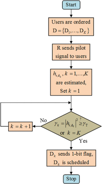

  

  Flowchart of the proposed MUSwiD user scheduling

• Centralized scheduling. In order to avoid any collusion, which may happen when multiple users send feedbacks, a centralized feedback collection method can be used. This method organizes the users to be orthogonal when they send feedbacks, such as time division multiplexing (TDM) where users are separated over time.

The multiuser switched diversity selection schemes proved themselves as a less complicated user selection schemes compared to the opportunistic scheduling from the number of channel estimations-wise. This happens on the expense of the system sum rate, which was shown in [35] to be compensated by significant savings in the CSI feedback load. The authors showed that the MUSwiD user selection schemes provide significant reduction of CSI feedback load at the cost of slight reduction in the achievable multiuser diversity gains, especially, at the low SNR values. This makes the MUSwiD selection schemes an attractive option for practical implementation in emerging mobile broadband communication systems.

3 Performance analysis

In this section, we evaluate closed-form approximations for the outage probability and average symbol error probability of the studied system. The channel capacity if also derived and numerically calculated in this section. The outage probability is a measure for the system performance and the possibility of the system to fall in outage. This is clear from the definition of the outage probability, which says that the system could get in outage once the SNR at the destination goes below a predetermined outage threshold γ _out or, equivalently the system is unable to achieve adequate reception. The possibility of the destination SNR to fall under a certain threshold exists in any communication system. In regard to deriving the ergodic capacity, as we are considering slowly varying fading channel model, this means that the coherence time of the channel is much larger than the data rate, and hence, the fading status remains constant over a large number of transmitted bits. This means that the average (i.e., ergodic) capacity of the channel could be a suitable measure for the best achievable capacity of the considered system links. In summary, the ergodic capacity we derived in this paper is valid under the assumption that the information symbol is long enough to ensure the long-term ergodic properties of the links.

3.1 Outage probability

In this section, we evaluate closed-form approximations for the outage probability for the i.n.i.d. and i.i.d. cases of users channels. The outage probability is defined as the probability that the SNR at the scheduled destination γ _up goes below a predetermined outage threshold γ _out , i.e., P _out =Pr[γ _up ≤γ _out ], where Pr[.] denotes the probability operation. Our results on the outage probability of the studied system are summarized in the following lemma and corollary.

Lemma 1

The outage probability for cognitive CSI-assisted AF MUSwiD relay system over Rayleigh fading channels is given for the case of i.n.i.d. users channels as

$$ \begin{aligned} P_{\mathsf{out}}&\simeq\sum_{i=0}^{K-1}\pi_{i}\lambda_{\mathsf{s,p}}\left\{\frac{\left(1-\exp\left(-\lambda_{\mathsf{s,p}} \gamma_{\mathsf{T}}\right)\right)}{\lambda_{\mathsf{s,p}}}+\sum_{k=0}^{K-1}(-1)^{k+1}\sum_{\substack{n_{0}<\ldots<n_{k}\\n(.)\neq i}}^{K-1}\right.\\&\quad\times\prod_{t=0}^{k}\frac{\left(1+\lambda_{2_{n_{t}}}\gamma_{\mathsf{T}}\right)^{-1}}{\Delta_{1}}-\left(1+\lambda_{2_{i}} \gamma_{\mathsf{out}}\right)^{-1}\\[-4pt] &\quad\times\left[{\vphantom{\sum_{\substack{n_{0}<\ldots<n_{k}\\n(.)\neq i}}^{K-1}}}\frac{\left(1-\exp\left(-\left(\lambda_{1}\gamma_{\mathsf{out}}+\lambda_{\mathsf{s,p}}\right) \gamma_{\mathsf{T}}\right)\right)}{\lambda_{1}\gamma_{\mathsf{out}}+\lambda_{\mathsf{s,p}}}+\sum_{k=0}^{K-1}(-1)^{k+1}\right.\\[-4pt] &\quad\left.\left.\times\sum_{\substack{n_{0}<\ldots<n_{k}\\n(.)\neq i}}^{K-1}\prod_{t=0}^{k}\frac{\left(1-\exp\left(-\Delta_{1}\gamma_{\mathsf{T}}\right)\right)}{\left(1+\lambda_{2_{n_{t}}} \gamma_{\mathsf{T}}\right)\Delta_{1}}\right]\right\}\\[-4pt] &\quad+\sum_{l=0}^{K-1}\pi_{l}\lambda_{\mathsf{s,p}}\left(\sum_{q=0}^{K}\frac{(-1)^{q}}{q!}\sum_{m_{1},\ldots,m_{q}}^{K} \prod_{z=1}^{q}\frac{\left(1-\exp\left(-\Delta_{1}\gamma_{\mathsf{T}}\right)\right)}{\left(1+\lambda_{2_{m_{z}}} \gamma_{\mathsf{T}}\right)\Delta_{1}}\right.\\[-4pt] &\quad+\sum_{w=0}^{K-1}\pi_{((l-w))_{K}}\left[(1+\lambda_{2_{l}} \gamma_{\mathsf{T}})^{-1}{\vphantom{\sum_{w=0}^{K-1}}}\right.\\[-4pt] &\quad\times\left\{\frac{\exp\left(-\left(\lambda_{1}\gamma_{\mathsf{T}}+\lambda_{\mathsf{s,p}}\right)\gamma_{\mathsf{T}}\right)} {\lambda_{1}\gamma_{\mathsf{T}}+\lambda_{\mathsf{s,p}}}+\sum_{p=0}^{w-1}(-1)^{p+1}\sum_{v_{0}<\ldots<v_{p}}^{w-1}\right.\\[-4pt] &\quad\left.\times\prod_{g=0}^{p}\frac{\exp\left(-\Delta_{2}\gamma_{\mathsf{T}}\right)}{\Delta_{3}\Delta_{2}}\right\}-\left(1+\lambda_{2_{l}} \gamma_{\mathsf{out}}\right)^{-1}\\[-4pt] &\quad\times\left\{\frac{\exp\left(-\left(\lambda_{1}\gamma_{\mathsf{out}}+\lambda_{\mathsf{s,p}}\right)\gamma_{\mathsf{T}}\right)} {\lambda_{1}\gamma_{\mathsf{out}}+\lambda_{\mathsf{s,p}}}+\sum_{p=0}^{w-1}(-1)^{p+1}\sum_{v_{0}<\ldots<v_{p}}^{w-1}\right.\\ &\;\;\,\left.\left.\left.\times\prod_{g=0}^{p}\frac{\exp\left(-\Delta_{4}\gamma_{\mathsf{T}}\right)}{\Delta_{3}\Delta_{4}}\right\}\right]\right), \end{aligned} $$

(2)

where Δ ₁=λ ₁ γ _T +λ _{s , p} , $\Delta _{2}=\sum _{u=0}^{p}\lambda _{2_{((l-w+v_{u}))_{K}}}+\lambda _{1}\gamma _{\mathsf {T}}+\lambda _{\mathsf {s,p}}\phantom {\dot {i}\!}$, $\Delta _{3}=1+\lambda _{2_{((l-w+v_{g}))_{K}}}\gamma _{\mathsf {T}}\phantom {\dot {i}\!}$, and $\Delta _{4}=\sum _{u=0}^{p}\lambda _{2_{((l-w+v_{u}))_{K}}}+\lambda _{1}\gamma _{\mathsf {out}}+\lambda _{\mathsf {s,p}}$.

Proof

Please, see Appendix. □

Corollary 1

The outage probability for cognitive CSI-assisted AF MUSwiD relay system over Rayleigh fading channels is given for the case of i.i.d. users channels (Ω _r,1=Ω _r,2=…=Ω _r,K =Ω _{r , d} ) as

$$ \begin{aligned} P_{\mathsf{out}}&\simeq\lambda_{\mathsf{s,p}}\left\{\sum_{g=0}^{K-1}\frac{{K-1 \choose g}(-1)^{g}}{\left(1+\lambda_{2}\gamma_{\mathsf{T}}\right)^{g}} \left[\frac{\left(1-\exp\left(-\left(g\lambda_{1}\gamma_{\mathsf{T}}+ \lambda_{\mathsf{s,p}}\right)\gamma_{\mathsf{T}}\right)\right)}{\left(g\lambda_{1}\gamma_{\mathsf{T}}+\lambda_{\mathsf{s,p}}\right)}\right.\right.\\[-4pt] &\quad\left.-\frac{\left(1-\exp\left(-\left(\left(\gamma_{\textsf{out}}+g\gamma_{\textsf{T}}\right)\lambda_{1}+\lambda_{\textsf{s,p}}\right) \gamma_{\textsf{T}}\right)\right)} {\left(1+\lambda_{2}\gamma_{\mathsf{out}}\right)\left(\left(\gamma_{\mathsf{out}}+g \gamma_{\mathsf{T}}\right)\lambda_{1}+\lambda_{\mathsf{s,p}}\right)}\right]\\[-4pt] &\quad+\sum_{j=0}^{K-1}\sum_{w=0}^{j}\frac{{j \choose w}(-1)^{w}}{\left(1+\lambda_{2}\gamma_{\mathsf{T}}\right)^{w}}\left[\frac{\exp\left(-\left((j+1)\lambda_{1}\gamma_{\mathsf{T}}+\lambda_{\mathsf{s,p}}\right)\gamma_{T}\right)} {\left(1+\lambda_{2}\gamma_{\mathsf{T}}\right)\left((j+1)\lambda_{1} \gamma_{\mathsf{T}}+\lambda_{\mathsf{s,p}}\right)}\right.\\[-4pt] &\quad\left.-\frac{\exp\left(-\left((\gamma_{\mathsf{out}}+j\gamma_{\mathsf{T}})\lambda_{1}+\lambda_{\mathsf{s,p}}\right)\gamma_{\textsf{T}}\right)} {\left(1+\lambda_{2}\gamma_{\mathsf{out}}\right)\left(\left(\gamma_{\mathsf{out}}+j\gamma_{\mathsf{T}}\right)\lambda_{1}+\lambda_{\mathsf{s,p}}\right)}\right]\\[-4pt] &\quad\left.+\sum_{q=0}^{K}\frac{{K \choose q}(-1)^{q}}{\left(1+\lambda_{2}\gamma_{\mathsf{T}}\right)^{q}}\frac{\exp\left(-\left(q\lambda_{1} \gamma_{\mathsf{T}}+\lambda_{\mathsf{s,p}}\right)\gamma_{\mathsf{T}}\right)}{\left(q\lambda_{1}\gamma_{\mathsf{T}}+\lambda_{\mathsf{s,p}}\right)}\right\}. \end{aligned} $$

(3)

Proof

In evaluating the outage probability in (3), the conditional CDF of γ _up is required to be obtained first. Based on the way the MUSwiD selection scheme works, this CDF can be written for the case of i.i.d. users channels as [36]

$$ {\begin{aligned} &F_{\gamma_{\mathsf{up}}}^{\text{MUSwiD}}\left(\gamma|h_{\mathsf{s,p}}\right)\\ &\quad=\left\{ \begin{array}{ll} \left[F_{\gamma^{\mathsf{up}}}\left(\gamma_{\mathsf{T}}|h_{\mathsf{s,p}}\right)\right]^{K-1}F_{\gamma^{\mathsf{up}}}\left(\gamma|h_{\mathsf{s,p}}\right), & \gamma<\gamma_{\mathsf{T}}; \\ \sum_{j=0}^{K-1}\left[F_{\gamma^{\mathsf{up}}}\left(\gamma|h_{\mathsf{s,p}}\right)-F_{\gamma^{\mathsf{up}}}\left(\gamma_{\mathsf{T}}|h_{\mathsf{s,p}}\right)\right]\\ \times\left[F_{\gamma^{\mathsf{up}}}\left(\gamma_{\mathsf{T}}|h_{\mathsf{s,p}}\right)\right]^{j}+\left[F_{\gamma^{\mathsf{up}}}\left(\gamma_{\mathsf{T}}|h_{\mathsf{s,p}}\right)\right]^{K}, & \gamma\geq\gamma_{\mathsf{T}}, \end{array} \right. \end{aligned}} $$

(4)

where $\phantom {\dot {i}\!}F_{\gamma ^{\mathsf {up}}}(\gamma |h_{\mathsf {s,p}})$ is the CDF of $\gamma ^{\mathsf {up}}_{k}$ conditioned on h _{s , p} , and it can be expressed for the case of i.i.d. first and second hop channels as

$$\begin{array}{*{20}l} F_{\gamma^{\mathsf{up}}_{k}}\left(\gamma|h_{\mathsf{s,p}}\right)=1-\frac{\exp\left(-\lambda_{1}\gamma|h_{\mathsf{s,p}}|^{2}\right)}{\left(1+\lambda_{2}\gamma\right)}, \end{array} $$

(5)

where λ ₁ is as defined in the Appendix and $\lambda _{2}=\Omega _{{\mathsf {r,p}}}\Big /\left (\Omega _{{\mathsf {r,d}}}\frac {\mathcal {I}_{\mathsf {p}}}{N_{0}}\right)$. Upon substituting (5) in (4) and following the same procedure as in the Appendix, we get the result in (3). □

Now, we derive the outage probability for the MUSwiDps selection scheme. Based on the way the MUSwiDps selection scheme works, the conditional CDF of γ _up can be written for the case of i.i.d. users channels as [36]

$$ \begin{aligned} &F_{\gamma_{\mathsf{up}}}^{\text{MUSwiDps}}\left(\gamma|h_{\mathsf{s,p}}\right)\\ &\quad=\left\{ \begin{array}{ll} \left[F_{\gamma^{\mathsf{up}}}(\gamma|h_{\mathsf{s,p}})\right]^{K-1}, & \text{\(\gamma<\gamma_{\mathsf{T}}\)}; \\ 1-\sum_{j=0}^{K-1}\left[F_{\gamma^{\mathsf{up}}}(\gamma_{\mathsf{T}}|h_{\mathsf{s,p}})\right]^{j} \left[1-F_{\gamma^{\mathsf{up}}}(\gamma|h_{\mathsf{s,p}})\right], & \text{\(\gamma\geq\gamma_{\mathsf{T}}\)}. \end{array} \right. \end{aligned} $$

(6)

Upon substituting (26) in (6) and following the same procedure as in the Appendix, the outage probability for the studied system with the MUSwiDps selection scheme can be evaluated in a closed-form approximation as

$$ \begin{aligned} P_{\mathsf{out}}&\simeq\lambda_{\mathsf{s,p}}\left\{\frac{\exp\left(-\lambda_{\mathsf{s,p}}\gamma_{\mathsf{T}}\right)}{\lambda_{\mathsf{s,p}}}-\sum_{j=0}^{K-1}\sum_{k=0}^{j}\frac{{j \choose k}(-1)^{k}}{\left(1+\lambda_{2}\gamma_{\mathsf{T}}\right)^{k}}\right.\\ &\quad\times\frac{\exp\left(-\left((k\gamma_{\mathsf{T}}+\gamma_{\mathsf{out}})\lambda_{1}+\lambda_{\mathsf{s,p}} \right)\gamma_{\mathsf{T}}\right)}{\left(1+\lambda_{2}\gamma_{\mathsf{out}}\right)\left((k\gamma_{\sf T}+\gamma_{\mathsf{out}})\lambda_{1}+\lambda_{\mathsf{s,p}}\right)}\\ &\quad\left.+\sum_{i=0}^{K}{K \choose i}(-1)^{i}\frac{\left(1-\exp\left(-\left(i\lambda_{1}\gamma_{\mathsf{out}}+\lambda_{\mathsf{s,p}}\right)\gamma_{\mathsf{T}}\right)\right)} {\left(1+\lambda_{2}\gamma_{\mathsf{out}}\right)^{i}\left(i\lambda_{1}\gamma_{\mathsf{out}}+\lambda_{\mathsf{s,p}}\right)}\right\}. \end{aligned} $$

(7)

3.2 Average symbol error probability

In this section, we evaluate closed-form approximations for the SEP for the i.n.i.d. and i.i.d. cases of users channels. The SEP can be expressed in terms of the CDF of γ _up , $F_{\gamma _{\mathsf {up}}}(\gamma)=P_{\mathsf {out}}(\gamma _{\mathsf {out}}=\gamma)$ as

$$\begin{array}{*{20}l} \text{SEP}\simeq\frac{a\sqrt{b}}{2\sqrt{\pi}}\int_{0}^{\infty}\frac{\exp\left(-b\gamma\right)}{\sqrt{\gamma}}F_{\gamma_{\mathsf{up}}}(\gamma) d\gamma, \end{array} $$

(8)

where a and b are modulation-specific constants. Our results on the SEP of the studied system are summarized in the following lemma and corollary.

Lemma 2

The SEP for cognitive CSI-assisted AF MUSwiD relay system is given for the case of i.n.i.d. users channels as

$$ \begin{aligned} \text{SEP}&\simeq\frac{a\sqrt{b}}{2\sqrt{\pi}}\lambda_{\mathsf{s,p}}\left\{\sum_{i=0}^{K-1}\pi_{i}\left(\frac{\sqrt{\pi}}{\sqrt{b} \lambda_{\mathsf{s,p}}}+\sum_{k=0}^{K-1}(-1)^{k+1}\sum_{\substack{n_{0}<\ldots<n_{k}\\n(.)\neq i}}^{K-1}\prod_{t=0}^{k}\right.\right.\\&\quad\times\frac{\left(1+\lambda_{2_{n_{t}}}\gamma_{\mathsf{T}}\right)^{-1}}{\vartheta_{1}} -\left[{\vphantom{\sum_{\substack{n_{0}<\ldots<n_{k}\\n(.)\neq i}}^{K-1}\prod_{t=0}^{k}\frac{\left(1-\exp\left(-\vartheta_{1}\gamma_{\mathsf{T}}\right)\right)} {\left(1+\lambda_{2_{n_{t}}}\gamma_{\mathsf{T}}\right)\vartheta_{1}}}}\left(-\frac{\lambda_{1}}{\lambda_{2_{i}}}+\lambda_{\mathsf{s,p}}\right)^{-1}\right.\\[-4pt] &\quad\times\Gamma(1/2)(\lambda_{2_{i}})^{-1/2}\left\{\exp\left(\frac{b}{\lambda_{2_{i}}}\right) \left(\Gamma\left(1/2,b/\lambda_{2_{i}}\right){\phantom{\frac{\lambda_{2_{i}}\lambda_{\mathsf{s,p}}}{\lambda_{1}}}}\right.\right.\\[-4pt] &\quad\left.\left.-\exp\left(-\left(\lambda_{\mathsf{s,p}}-\frac{\lambda_{1}}{\lambda_{2_{i}}}\right) \gamma_{\mathsf{T}}\right)\Gamma\left(1/2,(\lambda_{1}\gamma_{\mathsf{T}}+b)/\lambda_{2_{i}}\right)\right)\right.\\[-4pt] &\quad+\left(\frac{\lambda_{2_{i}}\lambda_{\mathsf{s,p}}}{\lambda_{1}}\right)^{-1/2} \exp\left(\frac{b\lambda_{\mathsf{s,p}}}{\lambda_{1}}\right)\left(\Gamma\left(1/2,(\lambda_{1}\gamma_{\mathsf{T}}+b) \lambda_{\mathsf{s,p}}/\lambda_{1}\right){\vphantom{\sum_{i=0}^{K-1}}}\right.\\[-4pt] &\quad\left.\left.{\vphantom{\sum_{i=0}^{K-1}}}-\Gamma\left(1/2,b\lambda_{\mathsf{s,p}}/\lambda_{1}\right)\right)\right\}+\sum_{k=0}^{K-1}(-1)^{k+1}\\[-4pt] &\quad\left.\left.\times\sum_{\substack{n_{0}<\ldots<n_{k}\\n(.)\neq i}}^{K-1}\prod_{t=0}^{k}\frac{\left(1-\exp\left(-\vartheta_{1}\gamma_{\mathsf{T}}\right)\right)} {\left(1+\lambda_{2_{n_{t}}}\gamma_{\mathsf{T}}\right)\vartheta_{1}}\right]\right)+\sum_{l=0}^{K-1}\pi_{l}\left(\sum_{q=0}^{K} \frac{(-1)^{q}}{q!}\right.\\[-4pt] &\quad\times\sum_{m_{1},\ldots,m_{q}}^{K}\prod_{z=1}^{q}\frac{\exp\left(-\vartheta_{1}\gamma_{\mathsf{T}}\right)} {\left(1+\lambda_{2_{m_{z}}}\gamma_{\mathsf{T}}\right)\vartheta_{1}}+\sum_{w=0}^{K-1}\pi_{((l-w))_{K}}\\[-4pt] &\quad\times\left[\left(1+\lambda_{2_{l}}\gamma_{\mathsf{T}}\right)^{-1}\left\{\frac{\exp\left(-\vartheta_{1}\right)} {\vartheta_{1}}+\sum_{p=0}^{w-1}(-1)^{p+1}\sum_{v_{0},\ldots,v_{p}}^{w-1}\prod_{g=0}^{p}\right.\right.\\[-4pt] &\quad\left.\times\frac{\exp\left(-\vartheta_{3}\gamma_{\mathsf{T}}\right)} {\left(1+\lambda_{2_{((l-w+v_{g}))_{K}}}\gamma_{\mathsf{T}}\right)\vartheta_{3}}\right\}- \left\{\left(-\frac{\lambda_{1}}{\lambda_{2_{l}}}+\lambda_{\mathsf{s,p}}\right)^{-1}\right.\\[-4pt] &\quad\times\Gamma(1/2)(\lambda_{l2})^{-1/2}\exp\left(-\lambda_{\mathsf{s,p}}\gamma_{\mathsf{T}}\right) \left(\exp\left(\frac{\lambda_{1}\gamma_{\mathsf{T}}+b}{\lambda_{2_{l}}}\right)\right.\\[-4pt] &\quad\times\Gamma \left(1/2,\left(\lambda_{1}\gamma_{\mathsf{T}}+b\right)/\lambda_{2_{l}}\right)-\left(\frac{\lambda_{2_{l}}\lambda_{\mathsf{s,p}}}{\lambda_{1}}\right)^{-1/2}\\[-4pt] &\quad\left.\left.\times\exp\left(\frac{(\lambda_{1}\gamma_{\mathsf{T}}+b)\lambda_{\mathsf{s,p}}}{\lambda_{1}}\right)\Gamma \left(1/2,(\lambda_{1}\gamma_{\mathsf{T}}+b)\lambda_{\mathsf{s,p}}/\lambda_{1}\right)\right){\vphantom{\left(-\frac{\lambda_{1}}{\lambda_{2_{l}}}+\lambda_{\mathsf{s,p}}\right)^{-1}}}\right\}\\[-4pt] &\quad+\sum_{p=0}^{w-1}(-1)^{p+1}\prod_{g=0}^{p}\frac{\exp\left(-\vartheta_{1}\gamma_{\mathsf{T}}\right)}{1+\lambda_{2_{((l-w+v_{g}))_{K}}}\gamma_{\mathsf{T}}}\\[-4pt] &\quad\times\left\{\left(-\frac{\lambda_{1}}{\lambda_{2_{l}}}+\lambda_{\mathsf{s,p}}\right)^{-1} \Gamma(1/2)(\lambda_{2_{l}})^{-1/2}\left(\vphantom{\sum_{p=0}^{w-1}}\exp\left(\frac{\lambda_{1}\gamma_{\mathsf{T}}+b}{\lambda_{2_{l}}}\right)\right.\right.\\[-4pt] &\quad\times\Gamma \left(1/2,\left(\lambda_{1}\gamma_{\mathsf{T}}+b\right)/\lambda_{2_{l}}\right)-\left(\frac{\lambda_{2_{l}}\lambda_{\mathsf{s,p}}}{\lambda_{1}}\right)^{-1/2}\\[-4pt] &\quad\left.\left.\left.\left.\left.\!\!\!\!{\vphantom{\sum_{p=0}^{w-1}}}\times\exp\left(\frac{(\lambda_{1}\gamma_{\mathsf{T}}+b)\lambda_{\mathsf{s,p}}}{\lambda_{1}}\right)\Gamma \left(1/2,(\lambda_{1}\gamma_{\mathsf{T}}+b)\lambda_{\mathsf{s,p}}/\lambda_{1}\right)\!\right)\!\right\}{\vphantom{\sum_{\substack{n_{0}<\ldots<n_{k}\\n(.)\neq i}}^{K-1}}}\right]\right)\right\}, \end{aligned} $$

(9)

where Γ(.,.)is the incomplete gamma function defined in ([ 37 ], Eq. (8.350.2)), 𝜗 ₁ =λ ₁ γ _T +λ _{s , p} and 𝜗 ₃=2λ ₁ γ _T +λ _{s , p} .

By replacing γ _out with γ in (2) and using the partial fraction expansion and the integration in (8) and with the help of ([37], Eq. (3.361.2)) and ([37], Eq. (3.383.10)), we get the result in (9).

Corollary 2

The SEP for cognitive CSI-assisted AF MUSwiD relay system is given for the case of i.i.d. users channels as

$$ \begin{aligned} \text{SEP}&\simeq\frac{a\sqrt{b}}{2\sqrt{\pi}}\lambda_{\mathsf{s,p}}\left\{{\vphantom{\frac{\exp\left(\frac{\left(j\gamma_{\mathsf{T}}+\frac{\lambda_{\mathsf{s,p}}}{\lambda_{1}}\right)} {\left(\lambda_{1}\gamma_{{T}}+b\right)^{-1}}\right)}{\left(\lambda_{2}\left(j\lambda_{1}+\frac{\lambda_{{s,p}}}{\lambda_{1}}\right)\right)^{1/2}}}}\sum_{g=0}^{K-1}\frac{{K-1 \choose g}(-1)^{g}}{\left(1+\lambda_{2}\gamma_{\mathsf{T}}\right)^{g}}\left[{\vphantom{\left.\left.-\Gamma\left(1/2,\left(\lambda_{1} \gamma_{\mathsf{T}}+b\right)\left(g\lambda_{1}\gamma_{\sf T}+\lambda_{\mathsf{s,p}}\right)/\lambda_{1}\right){\vphantom{\sum_{g=0}^{K-1}}}\right){\vphantom{\frac{\exp\left(\frac{b\left(g\lambda_{1}\gamma_{\mathsf{T}}+\lambda_{\mathsf{s,p}}\right)} {\lambda_{1}}\right)}{\left(\lambda_{2}\left(g\lambda_{1}+\frac{\lambda_{\mathsf{s,p}}}{\lambda_{1}}\right)\right)^{1/2}}}}\right\}}}\frac{\sqrt{\pi}\left(1-\exp\left(-\left(g\lambda_{1}\gamma_{\mathsf{T}}+ \lambda_{\mathsf{s,p}}\right)\gamma_{\mathsf{T}}\right)\right)}{\sqrt{b}\left(g\lambda_{1}\gamma_{\mathsf{T}}+ \lambda_{\mathsf{s,p}}\right)}\right.\right.\\[-3pt] &\quad-\frac{\Gamma(1/2)(\lambda_{2})^{-1/2}}{\left(\left(-\frac{1}{\lambda_{2}}+g\gamma_{\mathsf{T}}\right) \lambda_{1}+\lambda_{\mathsf{s,p}}\right)}\times\left\{\exp\left(b/\lambda_{2}\right)\left(\Gamma\left(1/2,b/\lambda_{2}\right){\vphantom{\sum_{g=0}^{K-1}}}\right.\right.\\[-3pt] &\quad\left.-\exp\left(-\left(\left(g-\frac{1}{\lambda_{2}}\right)\lambda_{1} \gamma_{\mathsf{T}}+\lambda_{\sf s,p}\right)\gamma_{\mathsf{T}}\right)\Gamma\left(1/2,(\lambda_{1}\gamma_{\mathsf{T}}+b)/\lambda_{2}\right){\vphantom{{\vphantom{\sum_{g=0}^{K-1}}}}}\right)\\[-3pt] &\quad-\frac{\exp\left(\frac{b\left(g\lambda_{1}\gamma_{\mathsf{T}}+\lambda_{\mathsf{s,p}}\right)} {\lambda_{1}}\right)}{\left(\lambda_{2}\left(g\lambda_{1}+\frac{\lambda_{\mathsf{s,p}}}{\lambda_{1}}\right)\right)^{1/2}} \left(\Gamma\left(1/2,b\left(g\lambda_{1}\gamma_{\mathsf{T}}+\lambda_{\mathsf{s,p}}\right)/\lambda_{1}\right){\vphantom{\sum_{g=0}^{K-1}}}\right.\\[-3pt] &\quad\left.\left.\left.-\Gamma\left(1/2,\left(\lambda_{1} \gamma_{\mathsf{T}}+b\right)\left(g\lambda_{1}\gamma_{\sf T}+\lambda_{\mathsf{s,p}}\right)/\lambda_{1}\right){\vphantom{\sum_{g=0}^{K-1}}}\right){\vphantom{\frac{\exp\left(\frac{b\left(g\lambda_{1}\gamma_{\mathsf{T}}+\lambda_{\mathsf{s,p}}\right)} {\lambda_{1}}\right)}{\left(\lambda_{2}\left(g\lambda_{1}+\frac{\lambda_{\mathsf{s,p}}}{\lambda_{1}}\right)\right)^{1/2}}}}\right\}\right]\\[-3pt] &\quad+\sum_{j=0}^{K-1}\sum_{w=0}^{j}\frac{{j \choose w}(-1)^{w}}{\left(1+\lambda_{2}\gamma_{\mathsf{T}}\right)^{w}}\left[\frac{\sqrt{\pi}\exp\left(-\left((j+1)\lambda_{1}\gamma_{\mathsf{T}}+ \lambda_{\mathsf{s,p}}\right)\gamma_{\mathsf{T}}\right)}{\sqrt{b}\left(1+\lambda_{2}\gamma_{\mathsf{T}}\right)\left((j+1)\lambda_{1} \gamma_{\mathsf{T}}+\lambda_{\mathsf{s,p}}\right)}{\vphantom{\frac{\exp\left(\frac{\left(j\gamma_{\mathsf{T}}+\frac{\lambda_{\mathsf{s,p}}}{\lambda_{1}}\right)} {\left(\lambda_{1}\gamma_{{T}}+b\right)^{-1}}\right)}{\left(\lambda_{2}\left(j\lambda_{1}+\frac{\lambda_{{s,p}}}{\lambda_{1}}\right)\right)^{1/2}}}}\right.\\[-3pt] &\quad-\frac{\Gamma(1/2)(\lambda_{2})^{-1/2}\exp\left(-\left(j\lambda_{1}\gamma_{\mathsf{T}}+ \lambda_{\mathsf{s,p}}\right)\gamma_{\mathsf{T}}\right)}{\left(\left(-\frac{1}{\lambda_{2}}+j\gamma_{\mathsf{T}}\right) \lambda_{1}+\lambda_{\mathsf{s,p}}\right)}\\[-3pt] &\quad\times\left\{\exp\left(\frac{\lambda_{1}\gamma_{\mathsf{T}}+b}{\lambda_{2}}\right)\Gamma\left(1/2,\left(\lambda_{1} \gamma_{\mathsf{T}}+b\right)/\lambda_{2}\right){\vphantom{\frac{\exp\left(\frac{\left(j\gamma_{\mathsf{T}}+\frac{\lambda_{\mathsf{s,p}}}{\lambda_{1}}\right)} {\left(\lambda_{1}\gamma_{{T}}+b\right)^{-1}}\right)}{\left(\lambda_{2}\left(j\lambda_{1}+\frac{\lambda_{{s,p}}}{\lambda_{1}}\right)\right)^{1/2}}}}{\vphantom{\frac{\exp\left(\frac{\left(j\gamma_{\mathsf{T}}+\frac{\lambda_{\mathsf{s,p}}}{\lambda_{1}}\right)} {\left(\lambda_{1}\gamma_{{T}}+b\right)^{-1}}\right)}{\left(\lambda_{2}\left(j\lambda_{1}+\frac{\lambda_{{s,p}}}{\lambda_{1}}\right)\right)^{1/2}}}}\right.\\[-3pt] &\quad\left.\left.-\frac{\exp\left(\frac{\left(j\gamma_{\mathsf{T}}+\frac{\lambda_{\mathsf{s,p}}}{\lambda_{1}}\right)} {\left(\lambda_{1}\gamma_{{T}}+b\right)^{-1}}\right)}{\left(\lambda_{2}\left(j\lambda_{1}+\frac{\lambda_{{s,p}}}{\lambda_{1}}\right)\right)^{1/2}} \Gamma\left(1/2,\frac{\left(j\gamma_{\mathsf{T}}+\frac{\lambda_{\mathsf{s,p}}}{\lambda_{1}}\right)} {\left(\lambda_{1}\gamma_{{T}}+b\right)^{-1}}\right)\right\}\right]\\[-3pt] &\quad\left.{\vphantom{\frac{\exp\left(\frac{\left(j\gamma_{\mathsf{T}}+\frac{\lambda_{\mathsf{s,p}}}{\lambda_{1}}\right)} {\left(\lambda_{1}\gamma_{{T}}+b\right)^{-1}}\right)}{\left(\lambda_{2}\left(j\lambda_{1}+\frac{\lambda_{{s,p}}}{\lambda_{1}}\right)\right)^{1/2}}}}+\sum_{q=0}^{K}\frac{{K \choose q}(-1)^{q}}{\left(1+\lambda_{2}\gamma_{\mathsf{T}}\right)^{q}}\frac{\sqrt{\pi}\exp\left(-\left(q\lambda_{1} \gamma_{\mathsf{T}}+\lambda_{\mathsf{s,p}}\right)\gamma_{\mathsf{T}}\right)}{\sqrt{b}\left(q\lambda_{1}\gamma_{\mathsf{T}}+\lambda_{\mathsf{s,p}}\right)}\right\}. \end{aligned} $$

(10)

By replacing γ _out with γ in (3) and using the partial fraction expansion and the integration in (8) and with the help of ([37], Eq. (3.361.2)) and ([37], Eq. (3.383.10)), we get the result in (10).

3.3 Ergodic channel capacity

In this section, we evaluate an expression for the ergodic channel capacity for the i.i.d. case of users channels. The ergodic capacity can be expressed in terms of the PDF of γ _up as

$$\begin{array}{*{20}l} {C}=\frac{1}{2\text{ln}(2)}\int_{0}^{\infty}\text{ln}(1+\gamma)f_{\gamma_{\mathsf{up}}}(\gamma) d\gamma. \end{array} $$

(11)

Our result on the ergodic capacity of the studied system is provided in the following lemma.

Lemma 3

The ergodic capacity for cognitive CSI-assisted AF MUSwiD relay system over Rayleigh fading channels is given for the case of i.i.d. users channels as

$$ \begin{aligned} {C}&\simeq\frac{1}{2\text{ln}(2)}\sum_{g=0}^{K-1}{K-1 \choose g}(-1)^{g}\left(1+\lambda_{2}\gamma_{\mathsf{T}}\right)^{-g}\left[{\vphantom{\sum_{g=0}^{K-1}}}\alpha \mathrm{ln(\lambda_{2})}(\lambda_{2}-1)^{-1}\right.\\ &\quad+\alpha\exp\left(-\left(g\lambda_{1}\gamma_{\sf T}+\lambda_{\mathsf{s,p}}\right)\gamma_{\sf T}\right)\\ &\quad\times\left\{-(\lambda_{1}\gamma_{\mathsf{T}}+\lambda_{2})\int_{0}^{\infty}\frac{\text{ln}(1+\gamma) \exp\left(-\lambda_{1}\gamma_{\mathsf{T}}\gamma\right)}{(1+\lambda_{2}\gamma)^{2}}d\gamma{\vphantom{\sum_{g=0}^{K-1}}}\right.\\ &\quad\left.-\lambda_{1}\lambda_{2}{\vphantom{\sum_{g=0}^{K-1}}} \gamma_{\mathsf{T}}\int_{0}^{\infty}\frac{\text{ln}(1+\gamma)\gamma\exp\left(-\lambda_{1}\gamma_{\mathsf{T}}\gamma\right)} {(1+\lambda_{2}\gamma)^{2}}d\gamma\right\}+\lambda_{1}\beta\\ &\quad\times\int_{0}^{\infty}\frac{\text{ln}(1+\gamma)}{(\lambda_{1}\gamma+g\lambda_{1}\gamma_{\mathsf{T}}+\lambda_{\sf s,p})}d\gamma+ \beta\exp\left(-\left(g\lambda_{1}\gamma_{\mathsf{T}}+\lambda_{\mathsf{s,p}}\right)\gamma_{\mathsf{T}}\right)\\ &\quad\times\left\{-(\lambda_{1})^{2}\gamma_{\mathsf{T}}\int_{0}^{\infty}\frac{\text{ln}(1+\gamma)\gamma\exp\left(-\lambda_{1}\gamma_{\mathsf{T}}\gamma\right)} {(\lambda_{1}\gamma+g\lambda_{1}\gamma_{\mathsf{T}}+\lambda_{\mathsf{s,p}})^{2}}d\gamma{\vphantom{\sum_{g=0}^{K-1}}}\right.\\ &\quad\left.\left.-\left(g(\lambda_{1})^{2}(\gamma_{\sf T})^{2}+\lambda_{1}\lambda_{\mathsf{s,p}}\gamma_{\mathsf{T}}+\lambda_{1}\right){\vphantom{\sum_{g=0}^{K-1}}}\right\}\right]+\sum_{j=0}^{K-1}\sum_{w=0}^{j}\frac{{j \choose w}(-1)^{w}}{\left(1+\lambda_{2}\gamma_{\mathsf{T}}\right)^{w}}\\ &\quad\times\left[-\exp\left(-\left(j\lambda_{1}\gamma_{\mathsf{T}}+\lambda_{\mathsf{s,p}}\right) \gamma_{\mathsf{T}}\right)\left(\alpha^{\prime}\left\{-(\lambda_{1}\gamma_{\mathsf{T}}+\lambda_{2}){\vphantom{\sum_{g=0}^{K-1}}}\right.\right.\right.\\ &\quad\times\int_{0}^{\infty}\frac{\text{ln}(1+\gamma)\exp\left(-\lambda_{1}\gamma_{\mathsf{T}}\gamma\right)} {(1+\lambda_{2}\gamma)^{2}}d\gamma-\lambda_{1}\lambda_{2}\gamma_{\mathsf{T}}\int_{0}^{\infty}\\ &\quad\left.{\vphantom{\sum_{g=0}^{K-1}}}\times\frac{\text{ln}(1+\gamma) \gamma\exp\left(-\lambda_{1}\gamma_{\mathsf{T}}\gamma\right)}{(1+\lambda_{2}\gamma)^{2}}d\gamma\right\}+\beta^{\prime}\left\{-(\lambda_{1})^{2} \gamma_{\mathsf{T}}{\vphantom{\sum_{g=0}^{K-1}}}\right.\\ &\quad\times\int_{0}^{\infty}\frac{\text{ln}(1+\gamma)\gamma\exp\left(-\lambda_{1}\gamma_{\mathsf{T}}\gamma\right)} {(\lambda_{1}\gamma+j\lambda_{1}\gamma_{\mathsf{T}}+\lambda_{\mathsf{s,p}})^{2}}d\gamma\\ &\quad-\left(j(\lambda_{1})^{2}(\gamma_{\mathsf{T}})^{2}+\lambda_{1}\lambda_{\mathsf{s,p}}\gamma_{\mathsf{T}}+\lambda_{1}\right)\int_{0}^{\infty}\\ &\quad\!\!\left.\left.\left.\times{\vphantom{\sum_{g=0}^{K-1}}}\frac{\text{ln}(1+\gamma)\exp\left(-\lambda_{1}\gamma_{\mathsf{T}}\gamma\right)} {(\lambda_{1}\gamma+j\lambda_{1}\gamma_{\mathsf{T}}+\lambda_{\mathsf{s,p}})^{2}}d\gamma\right\}\right)\right], \end{aligned} $$

(12)

where α, β, α ^′, and β ^′ are as given in the proof below. According to authors knowledge, the integrations in (12) have no closed-form solution. Hence, the ergodic channel capacity of the system is numerically evaluated.

Proof

Evaluating (12) requires the determination of the PDF of γ _up . By replacing γ _out with γ in (3) and using the partial fraction, the CDF $F_{\gamma _{\mathsf {up}}}(\gamma)$ can be written as

$$ \begin{aligned} F_{\gamma_{\sf up}}(\gamma)&\simeq\lambda_{\mathsf{s,p}}\left\{\sum_{g=0}^{K-1}\frac{{K-1 \choose g}(-1)^{g}}{\left(1+\lambda_{2}\gamma_{\mathsf{T}}\right)^{g}}\left[{\vphantom{\sum_{g=0}^{K-1}}} \left(1-\exp\left(-\left(g\lambda_{1}\gamma_{\mathsf{T}}+\lambda_{\mathsf{s,p}}\right)\gamma_{\mathsf{T}}\right)\right) \right.\right.\\ &\quad\times\left(g\lambda_{1}\gamma_{\mathsf{T}}+\lambda_{\mathsf{s,p}}\right)^{-1} -\alpha\frac{\left(1-\exp\left(-\left(\left(\gamma+g\gamma_{\mathsf{T}}\right)\lambda_{1} +\lambda_{\mathsf{s,p}}\right)\gamma_{\mathsf{T}}\right)\right)}{\left(1+\lambda_{2}\gamma\right)}\\ &\quad\left.-\beta\frac{\left(1-\exp\left(-\left(\left(\gamma+g\gamma_{\mathsf{T}}\right)\lambda_{1}+\lambda_{\mathsf{s,p}}\right)\gamma_{\mathsf{T}}\right)\right)} {\left(\lambda_{1}\gamma+g\lambda_{1}\gamma_{\mathsf{T}}+\lambda_{\mathsf{s,p}}\right)}\right]\\ &\quad+\sum_{j=0}^{K-1}\sum_{w=0}^{j}\frac{{j \choose w}(-1)^{w}}{\left(1+\lambda_{2}\gamma_{\mathsf{T}}\right)^{w}}\left[\frac{\exp\left(-\left((j+1)\lambda_{1}\gamma_{\mathsf{T}} +\lambda_{\mathsf{s,p}}\right)\gamma_{\mathsf{T}}\right)}{\left(1+\lambda_{2}\gamma_{\mathsf{T}}\right)\left((j+1)\lambda_{1} \gamma_{\mathsf{T}}+\lambda_{\mathsf{s,p}}\right)}\right.\\ &\quad-\exp\left(-\left(\left(j\lambda_{1}\gamma_{\mathsf{T}}\right) +\lambda_{\mathsf{s,p}}\right)\gamma_{\mathsf{T}}\right)\\ &\quad\left.\times\left(\exp\left(-\lambda_{1}\gamma_{\mathsf{T}}\gamma\right)\left\{\frac{\alpha^{\prime}} {\left(1+\lambda_{2}\gamma\right)}+\frac{\beta^{\prime}}{\left(\left(\gamma+j\gamma_{\mathsf{T}}\right)\lambda_{1} +\lambda_{\mathsf{s,p}}\right)}\right\}\right)\right]\\ &\quad\left.+\sum_{q=0}^{K}\frac{{K \choose q}(-1)^{q}}{\left(1+\lambda_{2}\gamma_{\mathsf{T}}\right)^{q}}\frac{\exp\left(-\left(q\lambda_{1} \gamma_{\mathsf{T}}+\lambda_{\mathsf{s,p}}\right)\gamma_{\mathsf{T}}\right)}{\left(q\lambda_{1} \gamma_{\mathsf{T}}+\lambda_{\mathsf{s,p}}\right)}\right\}. \end{aligned} $$

(13)

Solving for α, α ^′, β, and β ^′, we get $\alpha =\left (-\frac {\lambda _{1}}{\lambda _{2}}+g\lambda _{1}\gamma _{\mathsf {T}}+\lambda _{\mathsf {s,p}}\right)^{-1}$, $\beta =\left (1-\frac {(g\lambda _{1}\gamma _{\mathsf {T}}+\lambda _{\mathsf {s,p}})\lambda _{2}}{\lambda _{1}}\right)^{-1}$, and α ^′=α, β ^′=β with replacing g by j. By taking the derivative of (13) with respect to γ, the PDF $F_{\gamma _{\mathsf {up}}}(\gamma)$ can be obtained as

$$ \begin{aligned} f_{\gamma_{\mathsf{up}}}(\gamma)&\simeq\lambda_{\mathsf{s,p}}\left\{\sum_{g=0}^{K-1}\frac{{K-1 \choose g}(-1)^{g}}{\left(1+\lambda_{2}\gamma_{\mathsf{T}}\right)^{g}}\left[{\vphantom{\left.\left.+\frac{\lambda_{1}\exp\left(-\lambda_{1}\gamma_{\mathsf{T}}\gamma\right)} {\left(\lambda_{1}\gamma+g\lambda_{1}\gamma_{\mathsf{T}}+\lambda_{\mathsf{s,p}}\right)^{2}}\right\}\right)}}\alpha\left(\frac{\lambda_{2}} {\left(1+\lambda_{2}\gamma\right)^{2}}\right.\right.\right.\\ &\quad-\exp\left(-\left(g\lambda_{1}\gamma_{\mathsf{T}}+\lambda_{\mathsf{s,p}}\right)\gamma_{\mathsf{T}}\right) \left\{\frac{\lambda_{1}\gamma_{\mathsf{T}}\exp\left(-\lambda_{1}\gamma_{\mathsf{T}}\gamma\right)} {\left(1+\lambda_{2}\gamma\right)}\right.\\ &\quad\left.\left.+\frac{\lambda_{2}\exp\left(-\lambda_{1}\gamma_{\mathsf{T}}\gamma\right)} {\left(1+\lambda_{2}\gamma\right)^{2}}\right\}\right)+\beta\left(\frac{\lambda_{1}}{\left(\lambda_{1}\gamma+g\lambda_{1}\gamma_{\mathsf{T}}+\lambda_{\mathsf{s,p}}\right)^{2}}\right.\\ &\quad-\exp\left(-\left(g\lambda_{1}\gamma_{\mathsf{T}}+\lambda_{\mathsf{s,p}}\right)\gamma_{\mathsf{T}}\right)\left\{\frac{\lambda_{1}\gamma_{\mathsf{T}}\exp\left(-\lambda_{1}\gamma_{\mathsf{T}}\gamma\right)} {\left(\lambda_{1}\gamma+g\lambda_{1}\gamma_{\mathsf{T}}+\lambda_{\mathsf{s,p}}\right)}\right.\\ &\quad\left.\left.\left.+\frac{\lambda_{1}\exp\left(-\lambda_{1}\gamma_{\mathsf{T}}\gamma\right)} {\left(\lambda_{1}\gamma+g\lambda_{1}\gamma_{\mathsf{T}}+\lambda_{\mathsf{s,p}}\right)^{2}}\right\}\right)\right]+\sum_{j=0}^{K-1}\sum_{w=0}^{j}\frac{{j \choose w}(-1)^{w}}{\left(1+\lambda_{2}\gamma_{\mathsf{T}}\right)^{w}}\\ &\quad\times\left[{\vphantom{\sum_{j=0}^{K-1}}}-\exp\left(-\left(\left(j\lambda_{1}\gamma_{\mathsf{T}}\right)+\lambda_{\mathsf{s,p}}\right)\gamma_{\mathsf{T}}\right)\right.\\ &\quad\times\left(\alpha^{\prime}\left\{-\frac{\lambda_{1}\gamma_{\mathsf{T}}\exp\left(-\lambda_{1}\gamma_{\mathsf{T}}\gamma\right)} {\left(1+\lambda_{2}\gamma\right)}-\frac{\lambda_{2}\exp\left(-\lambda_{1}\gamma_{\mathsf{T}}\gamma\right)} {\left(1+\lambda_{2}\gamma\right)^{2}}\right\}\right.\\ &\quad\!\!\!\left.\left.\left.+\beta^{\prime}\left\{\!-\frac{\lambda_{1}\gamma_{\mathsf{T}}\exp\left(-\lambda_{1}\gamma_{\mathsf{T}}\gamma\right)} {\left(\lambda_{1}\gamma+j\lambda_{1}\gamma_{\mathsf{T}}+\lambda_{\mathsf{s,p}}\right)}\,-\,\frac{\lambda_{1}\exp\left(-\lambda_{1}\gamma_{\mathsf{T}}\gamma\right)} {\left(\lambda_{1}\gamma+j\lambda_{1}\gamma_{\mathsf{T}}+\lambda_{\mathsf{s,p}}\right)^{2}}\!\right\}\!\right)\!{\vphantom{\sum_{j=0}^{K-1}}}\right]\!\right\}. \end{aligned} $$

(14)

Upon substituting (14) in (11) and after some mathematical arrangements and with the help of ([37], Eq. (4.291.15)), we get the result in (12). □

4 Asymptotic performance analysis

Due to complexity of the achieved expressions in previous sections, it is hard to get more insights about system performance. Therefore, we see that it is important to derive simple expressions for the outage probability and ASEP at the high SNR values where more insights about the system behavior can be achieved. In this section, we evaluate the asymptotic outage performance of the studied system with the MUSwiD and MUSwiDps user selection schemes. At high SNR values, the outage probability can be expressed as $\phantom {\dot {i}\!}P_{\mathsf {out}}\approx (G_{\mathsf {c}}\text {SNR})^{-G_{\mathsf {d}}}$, where G _c denotes the coding gain of the system and G _d is the diversity order of the system [36]. The parameters on which the diversity order depends will affect the slope of the outage probability curves, and the parameters on which the coding gain depends will affect the position of the curves. In the upcoming analysis, the users are assumed to have identical channels.

As $\frac {\mathcal {I}_{\mathsf {p}}}{N_{0}} \rightarrow \infty$, the CDF in (26) simplifies to $F_{\gamma ^{\mathsf {up}}_{k}}\left (\gamma |h_{\mathsf {s,p}}\right)\approx \lambda _{1}|h_{\mathsf {s,p}}|^{2}\gamma$. Upon substituting this CDF in (4) and following the same procedure as in the Appendix, the outage probability at high SNR values can be evaluated with the help of ([37], Eq. (3.351.1)) and ([37], Eq. (3.351.2)) as

$$\begin{array}{*{20}l} P_{\mathsf{out}}^{\infty}&=\left(\gamma_{\mathsf{T}}\right)^{K-1}\left(\frac{\lambda_{1}}{\lambda_{\mathsf{s,p}}}\right)^{K}\gamma_{\mathsf{out}}\ \gamma\left(K+1,\lambda_{\mathsf{s,p}}\gamma_{\mathsf{T}}\right)\\ &\quad+\sum_{j=0}^{K-1}(\gamma_{\mathsf{T}})^{j}\left(\frac{\lambda_{1}}{\lambda_{\mathsf{s,p}}}\right)^{j+1}\Gamma\left(j+2,\lambda_{\mathsf{s,p}}\gamma_{\mathsf{T}}\right)\left(\gamma_{\mathsf{out}}-\gamma_{\mathsf{T}}\right)\\ &\quad+\left(\gamma_{\mathsf{T}}\right)^{K}\left(\frac{\lambda_{1}}{\lambda_{\mathsf{s,p}}}\right)^{K}\ \Gamma\left(K+1,\lambda_{\mathsf{s,p}}\gamma_{\mathsf{T}}\right), \end{array} $$

(15)

where γ(.,.) is the incomplete Gamma function defined in ([37], Eq. (8.350.1)).

One can notice that the result in (15) is dominated by the second term, which is still dominant when j=0. Hence, the outage probability for the studied system with the MUSwiD selection scheme can be evaluated at high SNR values as

$$\begin{array}{*{20}l} P_{\mathsf{out}}^{\infty}=\left(\frac{\lambda_{1}}{\lambda_{\mathsf{s,p}}}\right)\Gamma\left(2,\lambda_{\mathsf{s,p}}\gamma_{\mathsf{T}}\right)\left(\gamma_{\mathsf{out}}-\gamma_{\mathsf{T}}\right). \end{array} $$

(16)

Recalling that $\lambda _{1}=1\Big /\left (\Omega _{\mathsf {s,r}}\frac {\mathcal {I}_{\mathsf {p}}}{N_{0}}\right)$, (16) can be further simplified as

$$\begin{array}{*{20}l} P_{\mathsf{out}}^{\infty}=\left\{\frac{\Omega_{\mathsf{s,r}}\lambda_{\mathsf{s,p}}}{\Gamma\left(2,\lambda_{\mathsf{s,p}}\gamma_{\mathsf{T}}\right)\left(\gamma_{\mathsf{out}}-\gamma_{\mathsf{T}}\right)}\frac{\mathcal{I}_{\mathsf{p}}}{N_{0}}\right\}^{-1}. \end{array} $$

(17)

It is clear from (17) that the system with the MUSwiD selection scheme has a diversity order of 1 and a coding gain that is function of Ω _{s , r} , λ _{s , p} , γ _out , and γ _T .

The asymptotic SEP for the MUSwiD user selection scheme can be obtained by replacing γ _out by γ in (16) and then substituting the result in (8). Upon doing this and with the help of ([37], Eq. (3.351.3)), we get

$$\begin{array}{*{20}l} {\text{SEP}^{\infty}}=&\frac{a\sqrt{b}\lambda_{1}\Gamma\left(2,\lambda_{\mathsf{s,p}}\gamma_{\mathsf{T}}\right)}{2\sqrt{\pi}\lambda_{\mathsf{s,p}}}\left[\frac{\Gamma\left(\frac{3}{2}\right)}{b^{3/2}}-\frac{\Gamma\left(\frac{1}{2}\right)}{b^{1/2}}\gamma_{\mathsf{T}}\right]. \end{array} $$

(18)

Recalling that $\lambda _{1}=1\Big /\left (\Omega _{\mathsf {s,r}}\frac {\mathcal {I}_{\mathsf {p}}}{N_{0}}\right)$, (18) can be further simplified as

$$ \begin{aligned} {\text{SEP}^{\infty}}=&\left\{\left(\frac{a\sqrt{b}\Gamma\left(2,\lambda_{\mathsf{s,p}}\gamma_{\mathsf{T}}\right)}{2\sqrt{\pi}\lambda_{\mathsf{s,p}}\Omega_{\mathsf{s,r}}}\left[\frac{\Gamma\left(\frac{3}{2}\right)}{b^{3/2}}-\frac{\Gamma\left(\frac{1}{2}\right)}{b^{1/2}}\gamma_{\mathsf{T}}\right]\right)^{-1}\frac{\mathcal{I}_{\mathsf{p}}}{N_{0}}\right\}^{-1}. \end{aligned} $$

(19)

Now, we derive the asymptotic outage probability for the studied system with the MUSwiDps user selection scheme. Upon substituting the CDF $F_{\gamma ^{\mathsf {up}}_{k}}\left (\gamma |h_{\mathsf {s,p}}\right)\approx \lambda _{1}|h_{\mathsf {s,p}}|^{2}\gamma$ in (6) and following the same procedure as in the Appendix, the outage probability at high SNR values can be evaluated with the help of ([37], Eq. (3.351.1)) and ([37], Eq. (3.351.2)) as

$$\begin{array}{*{20}l} P_{\mathsf{out}}^{\infty}&=\left(\frac{\lambda_{1}}{\lambda_{\mathsf{s,p}}}\right)\Gamma\left(2,\lambda_{\mathsf{s,p}}\gamma_{\mathsf{T}}\right)\left(\gamma_{\mathsf{out}}-\gamma_{\mathsf{T}}\right)\\ &\quad+\gamma_{\mathsf{T}}\left(\frac{\lambda_{1}}{\lambda_{\mathsf{s,p}}}\right)^{2}\gamma_{\mathsf{out}}\Gamma\left(3,\lambda_{\mathsf{s,p}}\gamma_{\mathsf{T}}\right)\\ &\quad+\left(\frac{\lambda_{1}}{\lambda_{\mathsf{s,p}}}\right)^{K}(\gamma_{\mathsf{out}})^{K} \gamma\left(K+1,\lambda_{\mathsf{s,p}}\gamma_{\mathsf{T}}\right). \end{array} $$

(20)

Again, one can notice that the result in (20) is dominated by the first term, and hence, the outage probability for the studied system with the MUSwiDps selection scheme can be evaluated at high SNR values as

$$\begin{array}{*{20}l} P_{\mathsf{out}}^{\infty}=\left(\frac{\lambda_{1}}{\lambda_{\mathsf{s,p}}}\right)\Gamma\left(2,\lambda_{\mathsf{s,p}}\gamma_{\mathsf{T}}\right)\left(\gamma_{\mathsf{out}}-\gamma_{\mathsf{T}}\right). \end{array} $$

(21)

Recalling that $\lambda _{1}=1\Big /\left (\Omega _{\mathsf {s,r}}\frac {\mathcal {I}_{\mathsf {p}}}{N_{0}}\right)$, (21) can be further simplified as

$$\begin{array}{*{20}l} P_{\mathsf{out}}^{\infty}=\left\{\frac{\Omega_{\mathsf{s,r}}\lambda_{\mathsf{s,p}}}{\Gamma\left(2,\lambda_{\mathsf{s,p}}\gamma_{\mathsf{T}}\right)\left(\gamma_{\mathsf{out}}-\gamma_{\mathsf{T}}\right)}\frac{\mathcal{I}_{\mathsf{p}}}{N_{0}}\right\}^{-1}. \end{array} $$

(22)

It is clear that the asymptotic outage probability of the MUSwiDps user selection scheme is exactly the same as that of the MUSwiD scheme. Accordingly, the asymptotic SEP of the MUSwiDps scheme will be equal to that of the MUSwiD scheme as obtained in (19).

As can be seen from the results in (17) and (22), the coding gain of the system with the MUSwiD and MUSwiDps user selection schemes is affected by several parameters as Ω _{s , r} , λ _{s , p} , γ _out , and γ _T ; while the diversity order is constant at 1. This is clear in the numerical examples where all curves of different K asymptotically converge to the same behavior and result in a diversity order of 1. It is expected from the way the MUSwiD and MUSwiDps selection schemes operate that the gain achieved in system performance due to having more SU destinations to happen at the SNR values that are comparable to γ _T . As in this case, the switching rate will increase and the probability of having better users increases also. At the same time, as the asymptotic analysis is done at high SNR values, it is expected to have most of the users being acceptable the whole time and thus, the first checked user is being selected in the two selection schemes. This means all curves of different K asymptotically converge to same behavior, and this explains why the system with the two selection schemes has the same diversity order and the same coding gain as will be shown in numerical examples. In addition, it can be noticed from (17) and (22) that the diversity order of cognitive CSI-assisted AF MUSwiD relay network is the same as that of its non-cognitive counterpart. Specifically, it is equal to 1 and is independent of the primary network. It is worthwhile to mention here again that the importance of the proposed MUSwiD and MUSwiDps user selection schemes is in the reduced number of channel estimations and feedback load they require each transmission time compared to the opportunistic scheduling. Furthermore, from the asymptotic results, we conclude that the MUSwiD user selection schemes are inefficient at the range of high SNR values where the diversity order of the system becomes fixed and equal 1 when they are implemented. Accordingly, it is preferable to apply such low-complexity user scheduling schemes in systems that operate at the low range of SNR values as in the emerging mobile broadband communication systems. This fact about the applicability of the MUSwiD selection schemes was also proved and mentioned in [35].

The optimum switching threshold can be numerically calculated to minimize the e2e outage probability or symbol error probability. Due to complexity of the achieved expressions, any further manipulation with them to find the optimum threshold will increase the system complexity. Alternatively, we present here a simple method that can be used to get approximate but accurate values of the optimum switching threshold. In general, a good choice of the switching threshold is to have it near the average value of the e2e SNR, which can be upper bounded by the minimum of its two hops. Therefore, the optimum switching threshold can be calculated using $\text {min}\left (\frac {\frac {\mathcal {I}_{\mathsf {p}}}{N_{0}}|h_{\mathsf {s,r}}|^{2}} {|h_{{\mathsf {s,p}}}|^{2}},\frac {\frac {\mathcal {I}_{\mathsf {p}}}{N_{0}}|h_{{\mathsf {r}},k}|^{2}}{|h_{\mathsf {r,p}}|^{2}}\right)$. This method give excellent results as will be seen in the coming section.

5 Simulation and numerical results

In this section, we illustrate the validity of the achieved analytical and asymptotic expressions via a comparison with Monte-Carlo simulations. We also provide some numerical examples to show the effect of some system parameters such as number of users, switching threshold, and outage threshold on the system performance.

Figure 3 portrays the outage probability versus SNR for the studied system with the MUSwiD selection scheme for different number of users K. It is clear from this figure that the asymptotic results perfectly converge to the analytical results as well as the exact ones. Also, it is obvious that the used bound on the e2e SNR is indeed very tight; especially, at the high SNR region. Furthermore, we can see from this figure that the MUSwiD selection scheme has nearly the same performance as the best-user selection scheme for very low SNR region; whereas, as we go further in increasing SNR, the best-user selection scheme is clearly outperforming the MUSwiD scheme, as expected. In addition, we can see from this figure that for the MUSwiD scheme as K increases, the system performance becomes more enhanced; especially, at the range of SNR values that are comparable to the switching threshold γ _T . More importantly, for K=2, 3, and 4, it is obvious that at both low and high SNR values, all curves asymptotically converge to the same behavior and no gain is achieved in system performance with having more users. This is expected since when γ _T takes values much smaller or much larger than the average SNR, the system asymptotically converges to the case of two users, and hence, having more users will have no effect on the system performance. Also, it is clear that the curves in this figure greatly match the asymptotic or high SNR results where the diversity order was shown to be constant and equal 1. This shows that the MUSwiD and MUSwiDps selection schemes are inefficient at the range of high SNR values where the diversity order is noticeably degraded when they are implemented. Finally, the effectiveness of the MUSwiD and MUSwiDps schemes is in the reduction of CSI feedback load they offer compared to the opportunistic scheduling. In order to achieve this effectiveness with a slight reduction in the multiuser diversity gain, these user selection schemes should be implemented in the range of low SNR values such as in emerging mobile broadband communications systems.

Fig. 3

Outage probability vs SNR of cognitive AF relay network with MUSwiD user selection scheme for different values of K and Ω _{s , p} =30, and Ω _{s , r} =0.8, Ω _{r , p} =0.1, Ω _r,k =0.7 for k=1,…,4

Figure 4 studies the outage performance versus SNR for the studied system with the MUSwiD and MUSwiDps user selection schemes for different values of first hop power Ω _{s , r} . As can be seen from this figure, the MUSwiD and MUSwiDps selection schemes behave exactly the same in such kind of systems. Also, it is clear from the asymptotic results of this figure that the MUSwiD and MUSwiDps schemes have the same diversity order and the same coding gain. Finally, as Ω _{s , r} increases, the coding gain increases and better the achieved performance.

Fig. 4

Outage probability vs SNR of cognitive AF relay network with MUSwiD and MUSwiDps user selection schemes for different values of Ω _{s , r} and Ω _{s , p} =95, Ω _{r , p} =0.97, Ω _r,k =1 for k=1,2

Figure 5 shows the outage performance versus outage threshold for the studied system with the MUSwiD selection scheme for different values of SNR $\mathcal {I}_{\mathsf {p}}/N_{0}$. As expected, as γ _out increases, the worse the achieved performance. Also, it is obvious from this figure that the best performance is achieved at the largest value of SNR.

Fig. 5

Outage probability vs outage threshold of cognitive AF relay network with MUSwiD user selection scheme for different values of $\mathcal {I}_{\mathsf {p}}/N_{0}$ and Ω _{s , p} =60, and Ω _{s , r} =0.8, Ω _{r , p} =0.9, Ω _r,k =0.7 for k=1,…,6

Figure 6 illustrates the accuracy of the proposed method of finding the optimum switching threshold compared to the numerical method where the e2e outage probability is minimized. It is clear from this figure that the proposed method of finding approximate values for the optimum switching threshold γ _T gives a very close performance to that of the numerical method. This happens over a wide range of SNR values, which is 0–20 dB.

Fig. 6

Outage probability vs SNR of cognitive AF relay network with MUSwiD user selection scheme for different values of γ _T and Ω _{s , p} =7, and Ω _{s , r} =0.91, Ω _{r , p} =0.73, Ω _r,k =0.82 for k=1,2

Figure 7 studies the effects of the switching threshold γ _T and number of users K on the error probability performance of the studied system with the MUSwiD selection scheme. As can be seen from this figure, increasing K leads to a significant gain in system performance; especially, in the range of γ _T values that are comparable to the average value of $\gamma _{k}^{\mathsf {up}}$. On the other hand, as γ _T becomes much smaller or much larger than the average value of $\gamma _{k}^{\mathsf {up}}$, the improvement in performance decreases, as all curves asymptotically converge to the case of two users. This is due to the fact that, if the average value of $\gamma _{k}^{\mathsf {up}}$ is very small compared to γ _T , all users will be unacceptable most of the time. Whereas, if it is very high compared to γ _T , all users will be acceptable and one user will be scheduled most of the time. Thus, in both cases, having more users will not lead to any gain in the behavior.

Fig. 7

Symbol error probability vs switching threshold of cognitive AF relay network with MUSwiD user selection scheme for different values of K and Ω _{s , p} =20, and Ω _{s , r} =0.1, Ω _{r , p} =0.3, Ω _r,k =0.2 for k=1,…,5

Figure 8 shows the error probability performance versus number of users K for the studied system with the MUSwiD user selection scheme for different values of SNR $\mathcal {I}_{\mathsf {p}}/N_{0}$. It can be seen from this figure that the considered relay network still achieves performance gain and the error probability decreases when K increases, but the slope of the curves depends on the SNR values. Also, this figure validates the derived analytical expression of the average symbol error probability where a perfect fitting can be seen between the analytical result in (10) and its numerical solution that is achieved using (8).

Fig. 8

Symbol error probability vs number of users of cognitive AF relay network with MUSwiD user selection scheme for different values of $\mathcal {I}_{\mathsf {p}}/N_{0}$ and Ω _{s , p} =20, and Ω _{s , r} =0.8, Ω _{r , p} =0.6, Ω _r,k =0.8 for k=1,…,8

Figure 9 portrays the ergodic channel capacity versus SNR for the studied system with the MUSwiD user selection scheme for different values of Ω _{s , r} . Due to complexity of the derived expression of channel capacity, it is numerically calculated and plotted in this figure. As expected, the ergodic channel capacity enhances as the quality of first hop channel enhances.

Fig. 9

Channel capacity vs SNR of cognitive AF relay network with MUSwiD user selection scheme for different values of Ω _{s , r} and Ω _{s , p} =10, and Ω _{s , r} =1, Ω _{r , p} =2, Ω _r,k =3 for k=1,…,3

Figure 10 illustrates the validity of the PDF $F_{\gamma _{\mathsf {up}}}(\gamma)$ used in calculating the channel capacity. It is clear from this figure that the derived PDF of γ _up is a valid and a non-negative function. Also, we can see that the area under the curves of all considered cases in this figure is unity.

Fig. 10

The PDF $F_{\gamma _{\mathsf {up}}}(\gamma)$ vs γ of cognitive AF relay network with MUSwiD user selection scheme for different values of Ω _{s , p} and Ω _{s , r} =0.91, Ω _{r , p} =0.73, Ω _r,k =0.82 for k=1,2

Figure 11 illustrates the average number of channel estimations versus switching threshold γ _T for the MUSwiD and MUSwiDps user selection schemes in comparison with the opportunistic or best-user selection scheme for the case of four users. The average number of channel estimations for the MUSwiD and MUSwiDps schemes are provided in [38]. In this comparison, we assume that all channels are available for the relay or the central unit in order to conduct the selection among users. We can see from this figure that as the channels of all users are required for its operation, the opportunistic or best-user selection scheme is always of need for four channel estimations. On the other hand, we can see from this figure that the conventional MUSwiD selection scheme needs to estimate at most four channels because when the first three users are found unacceptable, the last checked user will be scheduled by the central unit regardless of its quality. Therefore, the MUSwiD scheme requires less channel estimations than the MUSwiDps scheme where in order to find the best user among all checked users, the channels of all users need to be estimated in the MUSwiDps scheme. Also, we can notice from this figure that as γ _T increases, the average number of channel estimations of users increases since it is more difficult to find a user with an acceptable quality.

Fig. 11

Average number of channel estimations of the MUSwiD and MUSwiDps user selection schemes in comparison with the best-user or opportunistic user selection scheme with K=4 and an average power/user path = 10 dB

6 Conclusions

In this paper, we evaluated the performance of a cognitive CSI-assisted AF relay network with the MUSwiD user selection scheme. Closed-form approximations for the outage probability and average symbol error probability were derived for the i.n.i.d. and i.i.d. cases of users channels. The ergodic channel capacity was also numerically evaluated. Furthermore, the system outage and error probability performances were evaluated at high SNR values where simple expressions for the outage probability, symbol error probability, diversity order, and coding gain were derived and analyzed for the MUSwiD and MUSwiDps user selection schemes. Monte-Carlo simulations proved the accuracy of the achieved analytical and asymptotic results. Findings illustrated that the proposed MUSwiD user selection schemes are efficient in the range of low SNR values, which makes them attractive options for practical implementation in emerging mobile broadband communication systems. In contrast, these selection schemes are inefficient in the range of high SNR values where the multiuser diversity gain is noticeably degraded when they are implemented. Furthermore, results illustrated that the gain achieved in performance due to having more users happens in the range of SNR values that are comparable to the switching threshold.

7 Endnotes

¹ Secondary users can know the channel information of the primary user by either a direct reception of pilot signals from a primary user [39], or by exchange of channel information between primary and secondary users through a band manager [40].

² This assumption is possible if the primary transmitter is located far from the secondary user [41], or the interference is represented in terms of noise when the primary transmitter’s signal is generated by random Gaussian codebooks [42].

³ In this paper, the switching threshold is numerically calculated to optimize the e2e outage probability. Also, a simple method is proposed in Section 4 to obtain approximate but accurate values of the optimum switching threshold.

⁴ The time duration of the feedback channel is not long, and hence, the MUSwiD scheduling scheme does not cause additional delay to the scheduling process [35].

8 Appendix

8.1 Proof of Lemma 1

In this Appendix, we derive the outage probability for the studied system when the secondary users have i.n.i.d. channels. In order to evaluate the outage probability, the CDF of γ _up is required to be obtained first. Herein, we first apply the conditional statistics on the fading channel from S to P. The CDF of $\gamma ^{\mathsf {up}}_{k}$ conditioned on h _{s , p} can be written as

$$ \begin{aligned} F_{\gamma^{\mathsf{up}}_{k}}\left(\gamma|h_{\mathsf{s,p}}\right)=1-\left(1-F_{\gamma_{1}}\left(\gamma|h_{\mathsf{s,p}}\right)\right) \left(1-F_{\gamma_{2_{k}}}\left(\gamma|h_{\mathsf{s,p}}\right)\right). \end{aligned} $$

(23)

It is easy to see that

$$\begin{array}{*{20}l} F_{\gamma_{1}}\left(\gamma|h_{\mathsf{s,p}}\right)=&1-\exp\left(-\lambda_{1}\gamma|h_{\mathsf{s,p}}|^{2}\right), \end{array} $$

(24)

$$\begin{array}{*{20}l} F_{\gamma_{2_{k}}}\left(\gamma|h_{\mathsf{s,p}}\right)=&\int_{0}^{\infty}F_{|h_{{\mathsf{r}},k}|^{2}}\left(\frac{N_{0}\gamma}{\mathcal{I}_{\mathsf{p}}}x\right)f_{|h_{\mathsf{r,p}}|^{2}}(x) dx \\ =&1-\left(1+\lambda_{2_{k}}\gamma\right)^{-1}, \end{array} $$

(25)

where $\lambda _{1}=1\Big /\left (\Omega _{\mathsf {s,r}}\frac {\mathcal {I}_{\mathsf {p}}}{N_{0}}\right)$ and $\lambda _{2_{k}}=\Omega _{\mathsf {r,p}}/\left (\Omega _{{\mathsf {r}},k}\frac {\mathcal {I}_{\mathsf {p}}}{N_{0}}\right)$.

Upon substituting (24) and (25) in (23), we get

$$\begin{array}{*{20}l} F_{\gamma^{\mathsf{up}}_{k}}\left(\gamma|h_{\mathsf{s,p}}\right)=1-\frac{\exp\left(-\lambda_{1}\gamma|h_{\mathsf{s,p}}|^{2}\right)}{\left(1+\lambda_{2_{k}}\gamma\right)}. \end{array} $$

(26)

Base on the way the MUSwiD selection scheme works, the conditional CDF at the output of this scheme can be written as [36]

$$ \begin{aligned} &F_{\gamma_{\mathsf{up}}}^{\text{MUSwiD}}\left(\gamma|h_{\mathsf{s,p}}\right)\\ &\quad=\left\{ \begin{array}{ll} \sum_{i=0}^{K-1}\pi_{i}F_{\gamma^{\mathsf{up}}_{i}}(\gamma|h_{\mathsf{s,p}})\prod^{K-1}_{\substack{k=0\\ k\neq{i}}}F_{\gamma^{\mathsf{up}}_{k}}(\gamma_{\mathsf{T}}|h_{\mathsf{s,p}}), & \gamma<\gamma_{\mathsf{T}}; \\ \sum_{l=0}^{K-1}\pi_{l}\bigg(\prod_{q=1}^{K}F_{\gamma^{\mathsf{up}}_{q}}(\gamma_{\mathsf{T}}|h_{\mathsf{s,p}})\\+\sum_{w=0}^{K-1}\pi_{((l-w))_{K}}\ \bigg[F_{\gamma^{\mathsf{up}}_{l}}(\gamma|h_{\mathsf{s,p}})-F_{\gamma^{\mathsf{up}}_{l}}(\gamma_{\mathsf{T}}|h_{\mathsf{s,p}})\bigg]\\ \times\prod_{p=0}^{w-1}F_{\gamma^{\mathsf{up}}_{((l-w+p))_{K}}}(\gamma_{\mathsf{T}}|h_{\mathsf{s,p}})\bigg),\ & \gamma\geq\gamma_{\mathsf{T}}, \\ \end{array} \right. \end{aligned} $$

(27)

where K is the number of SU destinations and γ _T is a predetermined switching threshold, π _i ,i=0,…,K−1 are the stationary distribution of a K-state Markov chain and it is the probability that the i ^th destination or user is chosen, and ((l−w)) _K denotes l−w modulo K. It is given by

$$ \begin{aligned} \pi_{i}&=\left[\sum_{j=0}^{K-1}\left(\frac{F_{\gamma^{\mathsf{up}}_{K-1}} (\gamma_{\mathsf{T}}|h_{\mathsf{s,p}})\left(1-F_{\gamma^{\mathsf{up}}_{j}} \left(\gamma_{\mathsf{T}}|h_{\mathsf{s,p}}\right)\right)}{F_{\gamma^{\mathsf{up}}_{j}}(\gamma_{\mathsf{T}}|h_{\mathsf{s,p}}) \left(1-F_{\gamma^{\mathsf{up}}_{K-1}}\left(\gamma_{\mathsf{T}}|h_{\mathsf{s,p}}\right)\right)}\right)\right]^{-1}\\ &\quad\times\frac{F_{\gamma^{\mathsf{up}}_{K-1}}(\gamma_{\mathsf{T}}|h_{\mathsf{s,p}})\left(1-F_{\gamma^{\mathsf{up}}_{i}} \left(\gamma_{\mathsf{T}}|h_{\mathsf{s,p}}\right)\right)}{F_{\gamma^{\mathsf{up}}_{i}} (\gamma_{\mathsf{T}}|h_{\mathsf{s,p}})\left(1-F_{\gamma^{\mathsf{up}}_{K-1}}\left(\gamma_{\mathsf{T}}|h_{\mathsf{s,p}}\right)\right)}. \end{aligned} $$

(28)

Upon substituting (26) in (27), we get

$$ \begin{aligned} &F_{\gamma_{\sf up}}\left(\gamma|h_{\mathsf{s,p}}\right)\\&=\left\{ \begin{array}{ll} \sum_{i=0}^{K-1}\pi_{i}\left(1-\frac{\exp\left(-\lambda_{1}\gamma|h_{\mathsf{s,p}}|^{2}\right)}{\left(1+\lambda_{2_{i}}\gamma\right)}\right)\underbrace{\prod^{K-1}_{\substack{k=0\\ k\neq{i}}}\left(1-\frac{\exp\left(-\lambda_{1}\gamma_{\mathsf{T}}|h_{\mathsf{s,p}}|^{2}\right)}{\left(1+\lambda_{2_{k}}\gamma_{\mathsf{T}}\right)}\right)}_{\mathcal{P}_{1}}, & \gamma<\gamma_{\mathsf{T}}; \\ \sum_{l=0}^{K-1}\pi_{l}\left\{\underbrace{\prod_{q=1}^{K}\left(1-\frac{\exp\left(-\lambda_{1}\gamma_{\mathsf{T}}|h_{\mathsf{s,p}}|^{2}\right)}{\left(1+\lambda_{2_{q}}\gamma_{\mathsf{T}}\right)}\right)}_{\mathcal{P}_{2}}\right.\\ +\sum_{w=0}^{K-1}\pi_{((l-w))_{K}} \left[\left(1-\frac{\exp\left(-\lambda_{1}\gamma|h_{\mathsf{s,p}}|^{2}\right)}{\left(1+\lambda_{2_{l}}\gamma\right)}\right)-\left(1-\frac{\exp\left(-\lambda_{1}\gamma_{\mathsf{T}}|h_{\mathsf{s,p}}|^{2}\right)}{\left(1+\lambda_{2_{l}}\gamma_{\mathsf{T}}\right)}\right)\right]\\ \left.\times\underbrace{\prod_{p=0}^{w-1}\left(1-\frac{\exp\left(-\lambda_{1}\gamma_{\mathsf{T}}|h_{\mathsf{s,p}}|^{2}\right)}{\left(1+\lambda_{2_{((l-w+p))_{K}}}\gamma_{\mathsf{T}}\right)}\right)}_{\mathcal{P}_{3}}\right\}, & \gamma\geq\gamma_{\mathsf{T}}. \\ \end{array} \right. \end{aligned} $$

(29)

With the help of the product identities in [43] and [20], the terms $\mathcal {P}_{1}$, $\mathcal {P}_{2}$, and $\mathcal {P}_{3}$ in (29) can be simplified as follows:

$$\begin{array}{*{20}l} \mathcal{P}_{1}&=1+\sum_{k=0}^{K-1}(-1)^{k+1}\sum_{\substack{n_{0}<\ldots<n_{k}\\ n_{(.)}\neq{i}}}^{K-1}\prod_{t=0}^{k}\left(1+\lambda_{2_{n_{t}}}\gamma_{\mathsf{T}}\right)^{-1}\\&\quad\times\exp\left(-\lambda_{1}\gamma_{\mathsf{T}}|h_{\mathsf{s,p}}|^{2}\right), \end{array} $$

(30)

where $\sum _{\substack {n_{0}<\ldots <n_{k}\\ n_{(.)}\neq {i}}}^{K-1}$ is a short-hand notation for $\sum _{\substack {n_{0}=0\\ n_{0}\neq {i}}}^{K-k-1}\sum _{\substack {n_{1}=n_{0}+1\\ n_{1}\neq {i}}}^{K-k}\ldots \sum _{\substack {n_{k}=n_{k-1}+1\\ n_{k}\neq {i}}}^{K-1}$.

$$\begin{array}{*{20}l} \mathcal{P}_{2}&=\sum_{q=0}^{K}\frac{(-1)^{q}}{q!}\sum_{m_{1},\ldots,m_{q}}^{K}\prod_{z=1}^{q} \left(1+\lambda_{2_{m_{z}}}\gamma_{\mathsf{T}}\right)^{-1}\\ &\quad\times\exp\left(-\lambda_{1}\gamma_{\mathsf{T}}|h_{\mathsf{s,p}}|^{2}\right), \end{array} $$

(31)

where $\sum _{m_{1},\ldots,m_{q}}^{K}$ is a short-hand notation for $\sum _{\substack {m_{1}=\ldots =m_{q}=1\\ m_{1}\neq \ldots \neq m_{q}}}^{K-k-1}$.

$$ \begin{aligned} \mathcal{P}_{3}&=1+\sum_{p=0}^{w-1}(-1)^{p+1}\sum_{v_{0}<\ldots<v_{p}}^{w-1}\prod_{g=0}^{p} \left(1+\lambda_{2_{((l-w+v_{g}))_{K}}}\gamma_{\mathsf{T}}\right)^{-1}\\&\quad\times\exp\left(-\lambda_{1}\gamma_{\mathsf{T}}|h_{\mathsf{s,p}}|^{2}\right), \end{aligned} $$

(32)

where $\sum _{v_{0}<\ldots <v_{p}}^{w-1}$ is a short-hand notation for $\sum _{v_{0}=0}^{w-p-1}\sum _{v_{1}=v_{0}+1}^{w-p}\ldots \sum _{v_{p}=v_{p-1}+1}^{w-1}$.

Up to now, the outage probability can be expressed as

$$\begin{array}{*{20}l} P_{\mathsf{out}}\simeq\int_{0}^{\infty}F_{\gamma_{\mathsf{up}}}\left(\gamma|h_{\mathsf{s,p}}\right)f_{|h_{\mathsf{s,p}}|^{2}}(y) dy. \end{array} $$

(33)

Upon substituting (30), (31), and (32) in (29) and using (33), the outage probability can be evaluated in a closed-form approximation as in (2).

References

S Haykin, Cognitive radio: Brain-empowered wireless communications. IEEE J. Sel. Areas Commun. 23(2), 201–220 (2005).
A Goldsmith, S Jafar, I Maric, S Srinivasa, Breaking spectrum gridlock with cognitive radios: an information theoretic perspective. Proc. IEEE. 97(5), 894–914 (2009).
JN Laneman, DNC Tse, GW Wornell, Cooperative diversity in wireless networks: efficient protocals and outage behavior. IEEE Trans. Inf. Theory. 50(12), 3062–3080 (2004).
VNQ Bao, TQ Duong, C Tellambura, On the performance of cognitive underlay multihop networks with imperfect channel state information. IEEE Trans. Commun. 61(12), 4864–4873 (2013).
Y Guo, G Kang, N Zhang, W Zhou, P Zhang, Outage performance of relay-assisted cognitive-radio system under spectrum-sharing constraints. Elect. Lett. 46(2), 182–184 (2010).
J Lee, H Wang, JG Andrews, D Hong, Outage probability of cognitive relay networks with interference constraints. IEEE Trans. Wirel. Commun. 10(2), 390–395 (2011).
L Luo, P Zhang, G Zhang, J Qin, Outage performance for cognitive relay networks with underlay spectrum sharing. IEEE Commun. Lett. 15(7), 710–712 (2011).
Z Yan, X Zhang, W Wang, Exact outage performance of cognitive relay networks with maximum transmit power limits. IEEE Commun. Lett. 15(12), 1317–1319 (2011).
Z El-Moutaouakkil, K Tourki, KA Qaraqe, S Saoudi, in Proc. IEEE Veh. Technol. Conf. (VTC’12-Fall). Exact outage probability analysis for relay-aided underlay cognitive communications (IEEE, Canada, 2012), pp. 1–5.
JP Hong, B Hong, TW Ban, W Choi, On the cooperative diversity gain in underlay cognitive radio systems. IEEE Trans. Commun. 60(1), 209–219 (2012).
VNQ Bao, DT Tran, in Proc. The 2012 IEEE Int’l Conf. on Adv. Tech. for Commun. Performance analysis of cognitive underlay DF relay protocol with K th best partial relay selection (IEEE, Vietnam, 2012), pp. 130–135.
X Zhang, Z Yan, Y Gao, W Wang, On the study of outage performance for cognitive relay networks (CRN) with the Nth best-relay selection in Rayleigh-fading channels. IEEE Wireless Commun. Lett. 2(1), 110–113 (2013).
H Chamkhia, MO Hasna, R Hamila, SI Hussain, in Proc. IEEE Int’l Symp. on Personal, Indoor & Mobile Radio Commun. (PIMRC’12). Performance analysis of relay selection schemes in underlay cognitive networks with decode and forward relaying (IEEE, Australia, 2012), pp. 1552–1558.
D Li, Outage probability of cognitive radio networks with relay selection. IET Commun.5(18), 2730–2735 (2011).
M Xia, S Aïssa, Cooperative AF relaying in spectrum-sharing systems: performance analysis under average interference power constraints and Nakagami-m fading. IEEE Trans. Commun. 60(6), 170–176 (2012).
SI Hussain, M-S Alouini, K Qaraqe, M Hasna, in Proc. IEEE Int’l Conf. on Commun. (ICC’12). Reactive relay selection in underlay cognitive networks with fixed gain relays (IEEE, Canada, 2012), pp. 1784–1788.
KB Fredj, S Aïssa, Performance of amplify-and-forward systems with partial relay selection under spectrum-sharing constraints. IEEE Trans. Wirel. Commun. 11(2), 500–504 (2012).
J Chen, Z Li, J Si, H Huang, R Gao, Outage probability analysis of partial AF relay selection in spectrum-sharing scenario with multiple primary users. Elect. Lett. 48(19), 1211–1212 (2012).
H Ding, J Ge, DB da Costa, Z Jiang, Asymptotic analysis of cooperative diversity systems with relay selection in a spectrum-sharing scenario. IEEE Trans. Veh. Technol. 60(2), 457–472 (2011).
VNQ Bao, TQ Duong, DB da Costa, GC Alexandropoulos, A Nallanathan, Cognitive amplify-and-forward relaying with best relay selection in non-identical Rayleigh fading. IEEE Commun. Lett. 17(3), 475–478 (2013).
Z Yan, X Zhang, W Wang, in Proc. IEEE Wire. Commun. and Net. Conf. (WCNC’11). Outage performance of relay assisted hybrid overlay/underlay cognitive radio systems (IEEE, Mexico, 2011), pp. 1920–1925.
JB Kim, D Kim, Outage probability and achievable diversity order of opportunistic relaying in cognitive secondary radio networks. IEEE Trans. Commun. 60(9), 2456–2466 (2012).
DB da Costa, M Elkashlan, PL Yeoh, N Yang, MD Yacoub, in Proc. 23rd IEEE Int’l Symp. on Personal Indoor & Mobile Radio Commun. (PIMRC’12). Dual-hop cooperative spectrum sharing systems with multi-primary users and multi-secondary destinations over Nakagami-m fading (IEEE, Australia, 2012), pp. 1577–1581.
C Zhai, W Zhang, Adaptive spectrum leasing with secondary user scheduling in cognitive radio networks. IEEE Trans. Wirel. Commun. 12(7), 3388–3398 (2013).
FRV Guimarães, DB da Costa, TA Tsiftsis, CC Cavalcante, GK Karagiannidis, Multi-user and multi-relay cognitive radio networks under spectrum sharing constraints. IEEE Trans. Veh. Technol. 63(1), 433–439 (2014).
EEB Olivo, DPM Osorio, DB da Costa, JCSS Filho, in Proc. 24th IEEE Int’l Symp. on Personal Indoor & Mobile Radio Commun. (PIMRC’13). Outage analysis of a spectrally efficient scheme for multiuser cognitive relaying networks with spectrum sharing constraints (IEEE, UK, 2013), pp. 997–1001.
Y Huang, F Al-Qahtani, C Zhong, Q Wu, in Proc. 2013 IEEE Int’l Conf. on Wireless Communications and Signal Processing. Outage analysis of spectrum sharing relay systems with multi-secondary destinations in the presence of primary user’s interference (IEEE, China, 2013), pp. 1–6.
AH Abd El-Malek, F Al-Qahtani, SA Zummo, H Alnuweiri, in Proc. IEEE Wire. Commun. and Net. Conf. (WCNC’15). MIMO multiuser cognitive relay network in spectrum sharing environment with antenna correlation over Rayleigh fading channels (IEEE, New Orleans, 2015), pp. 504–509.
J Yang, TQ Duong, M Elkashlan, X Lei, X Gao, in Proc. IEEE Int’l Conf. on Commun. (ICC’15). Multiuser scheduling for cognitive MIMO with channel estimation errors and feedback delay (IEEE, London, 2015), pp. 7737–7742.
B Holter, MS Alouini, GE Oien, HC Yang, in Proc. IEEE Veh. Technol. Conf, 3. Multiuser switched diversity transmission (IEEE, Los Angeles, 2004), pp. 2038–2043.
H Nam, MS Alouini, Multiuser switched diversity scheduling systems with per-user threshold. IEEE Trans. Commun. 58(5), 1321–1326 (2010).
H-C Yang, M-S Alouini, Performance analysis of multibranch switched diversity systems. IEEE Trans. Commun. 51(5), 782–794 (2003).
L Yang, M-S Alouini, Performance analysis of multiuser selection diversity. IEEE Trans. Veh. Technol. 55(6), 1848–1861 (2006).
Y Zhang, J Zheng, H-H Chen, Cognitive radio networks: architectures, protocols, and standards, 1st edn. (CRC Press, Taylor & Francis Group, 2010).
M Shaqfeh, H Alnuweiri, M-S Alouini, Multiuser switched diversity scheduling schemes. IEEE Trans. Commun. 60(9), 2499–2510 (2012).
MK Simon, M-S Alouini, Digital communication over fading channels, 2nd edn (Wiley, 2005).
IS Gradshteyn, IM Ryzhik, Tables of integrals, series and products, 6th edn (Acadamic Press, San Diago, 2000).
H-C Yang, M-S Alouini, Order statistics in wireless communications: diversity, adaptation, and scheduling in MIMO and OFDM Systems, 1st edn (Cambridge University Press, 2011).
T Ban, W Choi, B Jung, D Sung, Multi-user diversity in a spectrum sharing system. IEEE Trans. Wireless Commun. 8(1), 102–106 (2009).
A Ghasemi, E Sousa, Fundamental limits of spectrum-sharing in fading environments. IEEE Trans. Wireless Commun. 6(2), 649–658 (2007).
X Kang, Y Liang, A Nallanathan, in Proc. IEEE Veh. Technol. Conf. Optimal power allocation for fading channels in cognitive radio networks: delay-limited capacity and outage capacity (IEEE, Singapore, 2008), pp. 1544–1548.
R Etkin, A Parekh, D Tse, Spectrum sharing for unlicensed bands. IEEE J. Sel. Areas Commun. 25(3), 517–528 (2007).
PS Bithas, GK Karagiannidis, NC Sagias, PT Mathiopoulos, SA Kotsopoulos, GE Corazza, Performance analysis of a class of GSC receivers over nonidentical Weibull fading channels. IEEE Trans. Veh. Technol. 54(6), 1963–1970 (2005).
Acknowledgements
This work is supported by Deanship of Scientific Research (DSR) at King Fahd University of Petroleum & Minerals (KFUPM) through project #: RG1408-1,2.
Author information
Authors and Affiliations
Corresponding author
Ethics declarations
Competing interests
The authors’ declare that they have no competing interests.
Publisher’s Note
Springer Nature remains neutral with regard to jurisdictional claims in published maps and institutional affiliations.
Rights and permissions
Open Access This article is distributed under the terms of the Creative Commons Attribution 4.0 International License(http://creativecommons.org/licenses/by/4.0/), which permits unrestricted use, distribution, and reproduction in any medium, provided you give appropriate credit to the original author(s) and the source, provide a link to the Creative Commons license, and indicate if changes were made.
About this article
Cite this article
Salhab, A., Zummo, S. Performance analysis of cognitive AF relay networks with multiuser switched diversity in Rayleigh fading channels. J Wireless Com Network 2017, 133 (2017). https://doi.org/10.1186/s13638-017-0915-2
Received:
Accepted:
Published:
DOI: https://doi.org/10.1186/s13638-017-0915-2