Interference management with mismatched partial channel state information

Abstract

We study the fundamental limits of communications over multi-layer wireless networks where each node has only limited knowledge of the channel state information. In particular, we consider the scenario in which each source-destination pair has only enough information to perform optimally when other pairs do not interfere. Beyond that, the only other information available at each node is the global network connectivity. We propose a transmission strategy that solely relies on the available limited knowledge and combines coding with interference avoidance. We show that our proposed strategy goes well beyond the performance of interference avoidance techniques. We present an algebraic framework for the proposed transmission strategy based on which we provide a guarantee of the achievable rate. For several network topologies, we prove the optimality of our proposed strategy by providing information-theoretic outer-bounds.

1 Introduction

In dynamic wireless networks, optimizing system efficiency requires channel state information (CSI) in order to determine what resources are actually available. This information is acquired through feedback channel which is subject to several constraints such as delay, limited capacity, and locality. Consequently, in large-scale wireless networks, keeping track of the channel state information for making optimal decisions is typically infeasible due to the limitations of feedback channels and the significant overhead it introduces. Thus, in the absence of centralization of channel state information, nodes have limited local views of the network and make decentralized decisions based on their own local view of the network. The key question is how optimal decentralized decisions perform in comparison to the optimal centralized decisions.

In this paper, we consider multi-source multi-destination multi-layer wireless networks, and we seek fundamental limits of communications when sources have limited local views of the network. To model local views at wireless nodes, we consider the scenario in which each source-destination (S-D) pair has enough information to perform optimally when other pairs do not interfere. Beyond that, the only other information available at each node is the global network connectivity. We refer to this model of local network knowledge as 1-local view [1]. The motivation for this model stems from coordination protocols such as routing which are often employed in multi-hop networks to discover source-destination routes.

Our performance metric is normalized sum capacity defined in [2] which represents the maximum fraction of the sum capacity with full knowledge that can be always achieved when nodes have partial network knowledge. To better understand our objective, consider a multi-source multi-destination multi-layer wireless network. For each S-D pair, we define the induced subgraph by removing all other S-D pairs and the links that are not on a path between the chosen S-D pair. Our objective is to determine the minimum number of time slots T that is required for each S-D pair to reconstruct any transmission snapshot in their induced subgraph over the original network. Normalized sum capacity is simply equal to one over T.

Our main contributions are as follows. We propose an algebraic framework that defines a transmission scheme that only requires 1-local view at the nodes and combines coding with interference avoidance scheduling. The scheme is a combination of three main techniques: (1) per layer interference avoidance, (2) repetition coding to allow overhearing of the interference, and (3) network coding to allow interference neutralization.

We then characterize the achievable normalized sum rate of our proposed scheme and analyze its optimality for some classes of networks. We consider two-layer networks: (1) with two relays and any number of source-destination pairs, (2) with three source-destination pairs and three relays, and (3) with folded-chain structure (defined in Section 5). We also show that the gain from our proposed scheme over interference avoidance scheduling can be unbounded in L-nested folded-chain networks (defined in Section 5).

A related line of work was started by [3] which assumes wireless nodes are aware of the topology but not the channel state information. In this setting, all nodes have the same side information whereas in our work, nodes have partial and mismatched knowledge of the channel state information. The problem is then connected to index coding, and topological interference management scheme (TIM) is proposed. There are many results e.g., [4–9]) that follow a similar path of [3]. We generalize the problem to multi-hop networks and design our communication protocol accordingly, but TIM is designed for single-hop networks. Moreover, our formulation provides a continuous transition from no CSI to full CSI (by having more and more hops of knowledge) whereas [3] focuses only on the extreme case of no channel state information.

Many other models for imprecise network information have been considered for interference networks. These models range from having no channel state information at the sources [10–13], delayed channel state information [14–19], mismatched delayed channel state knowledge [20–22], or analog channel state feedback for fully connected interference channels [23]. Most of these works assume fully connected network or a small number of users. For networks with arbitrary connectivity, the first attempt to understand the role of limited network knowledge was initiated in [24, 25] in the context of single-layer networks. The authors used a message-passing abstraction of network protocols to formalize the notion of local view. The key result of [24, 25] is that local-view-based (decentralized) decisions can be either sum rate optimal or can be arbitrarily worse than the global-view (centralized) sum capacity. In this work, we focus on multi-layer setting and we show that several important additional ingredients are needed compared to the single-layer scenario.

It is worth noting that since each channel gain can range from zero to a maximum value, our formulation is similar to compound channels [26, 27] with one major difference. In the multi-terminal compound network formulations, all nodes are missing identical information about the channels in the network whereas in our formulation, the 1-local view results in asymmetric and mismatched information about channels at different nodes.

The rest of the paper is organized as follows. In Section 2, we introduce our network model and the new model for partial network knowledge. In Section 3 via a number of examples, we motivate our transmission strategies and the algebraic framework. In Section 4, we formally define the algebraic framework and we characterize the performance of the transmission strategy based on this framework. In Section 5, we prove the optimality of our strategies for several network topologies. Finally, Section 6 concludes the paper.

2 Problem formulation

In this section, we introduce our model for the wireless channel and the available network knowledge at the nodes. We also define the notion of normalized sum capacity which will be used as the performance metric for the strategies with partial network knowledge.

2.1 Network model and notations

We describe the two channel models we use in this paper, namely, the linear deterministic model and the Gaussian model. In both models, a network is represented by a directed graph

$$\begin{array}{*{20}l} \mathcal{G} = (\mathcal{V}, \mathcal{E},\{ w_{ij} \}_{(i,j) \in \mathcal{E}}) \end{array} $$

(1)

where $\mathcal {V}$ is the set of vertices representing nodes in the network, $\mathcal {E}$ is the set of directed edges representing links among these nodes, and $\{ w_{ij} \}_{(i,j) \in \mathcal {E}}$ represents the channel gains associated with the edges.

Out of the $|\mathcal {V}|$ nodes in the network, K nodes are sources and K nodes are destinations. We label these source and destination nodes by S _i s and D _i s respectively, i=1,2,…,K. The remaining $|\mathcal {V}|-2K$ nodes are relay nodes which facilitate the communication between sources and destinations. We can simply refer to a node in $\mathcal {V}$ as V _i , $i = 1,2,\ldots,|\mathcal {V}|$. In this work, we focus on two-layer networks.

The two channel models used in this paper are as follows:

• 1. The linear deterministic model [28]: In this model, there is a non-negative integer, w _ij =n _ij , associated with each link $(i,j) \in \mathcal {E}$ which represents its gain. Let q be the maximum of all the channel gains in this network. In the linear deterministic model, the channel input at node V _i at time t is denoted by

  $$\begin{array}{*{20}l} X_{\mathsf{V}_{i}}[\!t] = [\boldsymbol \!X_{\mathsf{V}_{i_{1}}}[\!t], X_{\mathsf{V}_{i_{2}}}[\!t], \ldots, X_{\mathsf{V}_{i_{q}}}[\!t] \!]^{T} \in \mathbb{F}_{2}^{q}. \end{array} $$

  (2)

  The received signal at node V _j at time t is denoted by

  $$\begin{array}{*{20}l} Y_{\mathsf{V}_{j}}[\!t] = [ \!Y_{\mathsf{V}_{j_{1}}}[\!t], Y_{\mathsf{V}_{j_{2}}}[\!t], \ldots, Y_{\mathsf{V}_{j_{q}}}[\!t]\! ]^{T} \in \mathbb{F}_{2}^{q}, \end{array} $$

  (3)

  and is given by

  $$ Y_{\mathsf{V}_{j}}[\!t] = \sum_{i: (i,j) \in \mathcal{E}}{\mathbf{S}^{q-n_{ij}} X_{\mathsf{V}_{i}}[\!t]}, $$

  (4)

  where S is the q×q shift matrix and the operations are in $\mathbb {F}_{2}^{q}$. If a link between V _i and V _j does not exist, we set n _ij to be zero.

• 2. The Gaussian model: In this model, the channel gain w _ij is denoted by $h_{ij} \in \mathbb {C}$. The channel input at node V _i at time t is denoted by $X_{\mathsf {V}_{i}}[t] \in \mathbb {C}$, and the received signal at node V _j at time t is denoted by $Y_{\mathsf {V}_{j}}[t] \in \mathbb {C}$ given by

  $$ Y_{\mathsf{V}_{j}}[\!t] = \sum_{i}{h_{ij} X_{\mathsf{V}_{i}}[\!t] + Z_{j}[\!t]}, $$

  (5)

  where Z _j [t] is the additive white complex Gaussian noise with unit variance. We also assume a power constraint of 1 at all nodes, i.e.,

  $$ {\lim}_{n\to\infty}\frac{1}{n} \mathbb{E}\left(\sum\limits_{t=1}^{n}{|X_{\mathsf{V}_{i}}[t]|^{2}}\right) \le 1. $$

  (6)

A route from a source S _i to a destination D _j is a set of nodes such that there exists an ordering of these nodes where the first one is S _i , the last one is D _j , and any two consecutive nodes in this ordering are connected by an edge in the graph.

Definition 1

Induced subgraph $\mathcal {G}_{ij}$ is a subgraph of $\mathcal {G}$ with its vertex set being the union of all routes (as defined above) from source S _i to a destination D _j , and its edge set being the subset of all edges in $\mathcal {G}$ between the vertices of $\mathcal {G}_{ij}$.

We say that S-D pair i and S-D j are non-interfering if $\mathcal {G}_{ii}$ and $\mathcal {G}_{jj}$ are two disjoint induced subgraphs of $\mathcal {G}$.

The in-degree function d _in(V _i ) is the number of in-coming edges connected to node V _i . Similarly, the out-degree function d _out(V _i ) is the number of out-going edges connected to node V _i . Note that the in-degree of a source and the out-degree of a destination are both equal to 0. The maximum degree of the nodes in $\mathcal {G}$ is defined as

$$ d_{\max} = \max_{i \in \{ 1,\ldots,|\mathcal{V}| \}} \left(d_{\text{in}}(\mathsf{V}_{i}), d_{\text{out}}(\mathsf{V}_{i}) \right). $$

(7)

2.2 Partial network knowledge model

We now describe our model for partial network knowledge that we refer to as 1-local view:

• All nodes have full knowledge of the network topology $(\mathcal {V},\mathcal {E})$ (i.e., they know which links are in $\mathcal {G}$, but not necessarily their channel gains). The network topology knowledge is denoted by side information SI;

• Each source, S _i , knows the gains of all the channels that are in $\mathcal {G}_{ii}$, i=1,2,…,K. This channel knowledge at a source is denoted by $\phantom {\dot {i}\!}L_{\mathsf {S}_{i}}$.

• Each node V _i (which is not a source) has the union of the information of all those sources that have a route to it, and this knowledge at node is denoted by $\phantom {\dot {i}\!}L_{\mathsf {V}_{i}}$.

This partial network knowledge is motivated by the following argument. Suppose a network with a single S-D pair and no interference. In such a network, one expects the S-D pair to be able to communicate optimally (or close to optimal) and our model guarantees this baseline performance. In fact, our model assumes the minimum knowledge needed at different nodes such that each S-D pair can communicate optimally in the absence of interference. Moreover, our assumption is backed by message passing algorithm which is how CSI is learned in wireless networks.

For a depiction, consider the network in Fig. 1a. Source S ₁ has the knowledge of the channel gains of the links that are denoted by solid arrows in Fig. 1a. On the other hand, relay A has the union of the information of sources S ₁ and S ₂. The partial knowledge of relay A is denoted by solid arrows in Fig. 1b.

Fig. 1

a The partial knowledge of the channel gains available at source S ₁ is denoted by solid arrows and b the partial knowledge of the channel gains available at relay A

Remark 1

Our formulation is a general version of compound channel formulation where nodes have mismatched and asymmetric lack of knowledge.

2.3 Performance metric

Our goal is to find out the minimum number of time slots such that all induced subgraphs can be reconstructed as if there is no interference. It turns out the aforementioned objective is closely related to the notion of normalized sum capacity introduced in [2]. Here, we define the notion of normalized sum capacity which is going to be our metric for evaluating network capacity with partial network knowledge. Intuitively, normalized sum capacity represents the maximum fraction of the sum capacity with full knowledge that can be achieved when nodes have partial network knowledge.

Consider the scenario in which source S _i wishes to reliably communicate message $\phantom {\dot {i}\!}\text {W}_{i} \in \{ 1,2,\ldots,2^{N R_{i}}\}$ to destination D _i during N uses of the channel, i=1,2,…,K. We assume that the messages are independent and chosen uniformly. For each source S _i , let message W _i be encoded as $X_{\mathsf {S}_{i}}^{N}\phantom {\dot {i}\!}$ using the encoding function $\phantom {\dot {i}\!}e_{i}(\text {W}_{i}|L_{\mathsf {S}_{i}},\mathsf {SI})$ which depends on the available local network knowledge, $L_{\mathsf {S}_{i}}\phantom {\dot {i}\!}$, and the global side information, SI.

Each relay in the network creates its input to the channel, $\phantom {\dot {i}\!}X_{\mathsf {V}_{i}}$, using the encoding function $\phantom {\dot {i}\!}f_{\mathsf {V}_{i}}[\!t]\left (Y_{\mathsf { V}_{i}}^{(t-1)}|L_{\mathsf {V}_{i}},\mathsf {SI}\right)$ which depends on the available network knowledge, $\phantom {\dot {i}\!}L_{\mathsf {V}_{i}}$, and the side information, SI, and all the previous received signals at the relay $\phantom {\dot {i}\!}Y_{\mathsf {V}_{i}}^{(t-1)} = \left [ Y_{\mathsf {V}_{i}}[1], Y_{\mathsf {V}_{i}}[\!2], \ldots, Y_{\mathsf {V}_{i}}[\!t-1]\! \right ]$. A relay strategy is defined as the union of all encoding functions used by the relays, $\phantom {\dot {i}\!}\{ f_{\mathsf {V}_{i}}[t](Y_{\mathsf {V}_{i}}^{(t-1)}|L_{\mathsf {V}_{i}},\mathsf {SI}) \}$, t=1,2,…,N and $\mathsf {V}_{i} \in \bigcup _{j=1}^{L-1}{\mathcal {V}_{j}}$.

Destination D _i is only interested in decoding W _i , and it will decode the message using the decoding function $\phantom {\dot {i}\!}\widehat {\text {W}}_{i} = d_{i}(Y_{\mathsf {D}_{i}}^{N} |L_{\mathsf {D}_{i}},\mathsf {SI})$ where $L_{\mathsf {D}_{i}}\phantom {\dot {i}\!}$ is destination D _i ’s network knowledge. We note that the local view can vary from node to node.

Definition 2

A Strategy $\mathcal {S}_{N}$ is defined as the set of: (1) all encoding functions at the sources, (2) all decoding functions at the destinations, and (3) the relay strategy for t=1,2,…,N, i.e.,

$$ \mathcal{S}_{N} = \left\{ \begin{array}{ll} e_{i}(\text{W}_{i}|L_{\mathsf{S}_{i}},\mathsf{SI}) & i = 1,2,\ldots,K \\ f_{\mathsf{V}_{i}}[\!t]\left(Y_{\mathsf{V}_{i}}^{(t-1)}|L_{\mathsf{ V}_{i}},\mathsf{SI}\right) & t=1,2,\ldots,N \\ & \text{and}\; \mathsf{V}_{i} \in \bigcup_{j=1}^{L-1}{\mathcal{V}_{j}} \\ d_{i}(Y_{\mathsf{D}_{i}}^{N} |L_{\mathsf{D}_{i}},\mathsf{SI}) & i = 1,2,\ldots,K \end{array} \right\}. $$

(8)

An error occurs when $\widehat {\text {W}}_{i} \neq \text {W}_{i}$, and we define the decoding error probability, λ _i , to be equal to $P(\widehat {\text {W}}_{i} \neq \text {W}_{i})$. A rate tuple (R ₁,R ₂,…,R _K ) is said to be achievable if there exists a set of strategies $\{ \mathcal {S}_{j} \}_{j=1}^{N}$ such that the decoding error probabilities λ ₁,λ ₂,…,λ _K go to zero as N→∞ for all network states consistent with the side information. Moreover, for S-D pair i, we denote the maximum achievable rate with full network knowledge by C _i . The sum capacity C _sum is the supremum of $\sum _{i=1}^{K}{R_{i}}$ over all possible encoding and decoding functions with full network knowledge.

We now define the normalized sum rate and the normalized sum capacity.

Definition 3

([2]) Normalized sum rate of α is said to be achievable if there exists a set of strategies $\{ \mathcal {S}_{j} \}_{j=1}^{N}$ such that following holds. As N goes to infinity, strategy $\mathcal {S}_{N}$ yields a sequence of codes having rates R _i at source S _i , i=1,…,K, satisfying

$$\sum_{i=1}^{K}{R_{i}} \ge \alpha C_{\text{sum}} -\tau $$

such that error probabilities at the destinations, λ ₁,⋯λ _K , go to zero for all the network states consistent with the side information and for a constant τ that is independent of the channel gains.

Definition 4

([2]) Normalized sum capacity α ^∗ is defined as the supremum of all achievable normalized sum rates α. Note that α ^∗∈ [0,1].

Remark 2

While the results of this paper may appear pessimistic, they are much like any other compound channel analysis which aims to optimize the worst case scenario. We adopted the normalized capacity as our metric which opens the door for exact (or near-exact) results for several cases as we will see in this paper. We view our current formulation as a step towards the general case, much like the commonly accepted methodology where channel state information is assumed known perfectly in first steps of a new problem (MIMO, interference channels, scaling laws), even though that assumption is almost never possible.

3 Motivating examples

Before diving into the main results, we use a sequence of examples to understand the mechanisms that allow us outperform interference avoidance with only 1-local view.

We first consider the single-layer network depicted in Fig. 2a. Using interference avoidance, we can create the induced subgraphs of all three S-D pairs as shown in Fig. 2b in three time slots. Thus, with interference avoidance, one can only achieve $\alpha =\frac {1}{3}$ which is the same as TDMA. However, we show that it is possible to reconstruct the three induced subgraphs in only two time slots and to achieve $\alpha =\frac {1}{2}$ with 1-local view.

Fig. 2

a A network in which coding is required to achieve the normalized sum capacity and b the induced subgraphs

Consider the linear deterministic model and the induced subgraphs of all three S-D pairs as shown in Fig. 2b. We show that any transmission strategy over these three induced subgraphs can be implemented in the original network by using only two time slots such that all nodes receive the same signal as if they were in the induced subgraphs. This would immediately imply that a normalized sum rate of $\frac {1}{2}$ is achievable¹.

To do so, we split the communication block into two time slots of equal length. Sources S ₁ and S ₂ transmit the same codewords as if they are in the induced subgraphs over first time slot. Destination D ₁ receives the same signal as it would have in its induced subgraph, and destination D ₃ receives interference from source S ₂.

Over second time slot, S ₃ transmits the same codeword as if it was in its induced subgraph and S ₂ repeats its transmit signal from the first time slot. Destination D ₂ receives its signal interference-free. Now, if destination D ₃ adds its received signals over the two time slots, it recovers its intended signal as depicted in Fig. 3. In other words, we used interference cancellation at destination D ₃. Therefore, all S-D pairs can effectively communicate interference-free over two time slots.

Fig. 3

Achievability strategy for the network depicted in Fig. 2

We can view this discussion in an algebraic framework. To each source S _i , we assign a transmit vector $\mathbf {T}_{\mathsf {S}_{i}}\phantom {\dot {i}\!}$ of size 2×1 where 2 corresponds to the number of time slots. If the entry at row t is equal to 1, then S _i communicates the codeword for D _i during time slot t, i=1,2,3, and t=1,2. In our example, we have

$$\begin{array}{*{20}l} \mathbf{T}_{\mathsf{S}_{1}} = \left(\begin{array}{c} 1 \\ 0 \end{array} \right), \quad \mathbf{T}_{\mathsf{S}_{2}} = \left(\begin{array}{c} 1 \\ 1 \end{array} \right), \quad \mathbf{T}_{\mathsf{S}_{3}} = \left(\begin{array}{c} 0 \\ 1 \end{array} \right). \end{array} $$

(9)

To each destination D _i , we assign a receive matrix $\mathbf {R}_{\mathsf {D}_{i}}\phantom {\dot {i}\!}$ of size 2×2 where each row corresponds to a time slot and each column corresponds to a source that has a route to destination D _i . More precisely, $\mathbf {R}_{\mathsf {D}_{i}}\phantom {\dot {i}\!}$ is formed by concatenating the transmit vectors of the sources that are connected to D _i . In our example, we have

$$\begin{array}{*{20}l} & \mathbf{R}_{\mathsf{D}_{1}} = \left(\mathbf{T}_{\mathsf{S}_{1}} \mathbf{T}_{\mathsf{S}_{3}} \right) = {t=1 \atop t=2} \overset{\mathsf{S}_{1}\quad \mathsf{S}_{3}} {\left(\begin{array}{cc} 1 &\quad 0 \\ 0 &\quad 1 \\ \end{array}\right),} \\ & \mathbf{R}_{\mathsf{D}_{2}} = {t=1 \atop t=2} \overset{\mathsf{S}_{1} \quad \mathsf{S}_{2}} {\left(\begin{array}{cc} 1 &\quad 1 \\ 0 &\quad 1 \\ \end{array}\right),} \quad \mathbf{R}_{\mathsf{D}_{3}} = {t=1 \atop t=2} \overset{\mathsf{S}_{2} \quad \mathsf{S}_{3}} {\left(\begin{array}{cc} 1 &\quad 0 \\ 1 &\quad 1 \\ \end{array}\right) }. \end{array} $$

(10)

From the receive matrices in (10), we can easily check whether each destination can recover its corresponding signal or not. For instance, from $\mathbf {R}_{\mathsf {D}_{1}}\phantom {\dot {i}\!}$, we know that in time slot 1, the signal from S ₁ is received interference-free. A similar story is true for the second pair and $\mathbf {R}_{\mathsf {D}_{2}}\phantom {\dot {i}\!}$. From $\mathbf {R}_{\mathsf {D}_{3}}\phantom {\dot {i}\!}$, we see that in time slot 2, the signal from S ₃ is received with interference from S ₂. However, with a linear row-operation, we can create a row where the only 1 appears in the column associated with S ₃. More precisely,

$$\begin{array}{*{20}l} \mathbf{R}_{\mathsf{D}_{3}}\left(1, : \right) \oplus \mathbf{R}_{\mathsf{D}_{3}}\left(2, : \right) = \overset{\mathsf{S}_{2} \quad \mathsf{S}_{3}} {\left(0 \quad 1\right)}. \end{array} $$

where $\mathbf {R}_{\mathsf {D}_{3}}\left (t, : \right)\phantom {\dot {i}\!}$ denotes row t of matrix $\mathbf {R}_{\mathsf {D}_{3}}\phantom {\dot {i}\!}$. Thus, each destination can recover its intended signal interference-free over two time slots. More precisely, we require

$$\begin{array}{*{20}l} \overset{\mathsf{S}_{i} \quad \mathsf{S}_{j}}{(1 \quad 0)} \in \text{rowspan}\left(\mathbf{R}_{\mathsf{D}_{i}} \right), \quad i,j \in \{ 1,2,3 \}, \quad j \neq i. \end{array} $$

(11)

This example illustrated that with only 1-local view, it is possible to reconstruct the three induced subgraphs in only two time slots using (repetition) coding at the sources and go beyond interference avoidance and TDMA. In the following example, we show that more sophisticated ideas are required to beat TDMA in multi-layer networks.

Consider the two-layer network of Fig. 4a. Under the linear deterministic model it is straightforward to see that by using interference avoidance or TDMA, it takes three time slots to reconstruct the induced subgraphs of Fig. 4b–d, which results in a normalized sum rate of $\alpha =\frac {1}{3}$.

Fig. 4

a A two-layer network in which we need to incorporate network coding to achieve the normalized sum capacity, b–d the induced subgraphs of S-D pairs 1, 2, and 3, respectively

We now show that using repetition coding at the sources and linear coding at the relays, it is possible to achieve α=1/2 and reconstruct the three induced subgraphs in only two time slots. This example was first presented in [1].

Consider any strategy for S-D pairs 1, 2, and 3 as illustrated in Fig. 4b–d. In the first layer, we implement the achievability strategy of Fig. 3 illustrated in Fig. 5. As it can be seen in this figure, at the end of the second time slot, each relay has access to the same received signal as if it was in the diamond networks of Fig. 4b–d.

Fig. 5

Achievability strategy for the first layer of the network in Fig. 4a

In the second layer during the first time slot, relays V ₁ and V ₂ transmit $X_{\mathsf {V}_{1}}^{1}$ and $X_{\mathsf { V}_{2}}^{1}$, respectively, whereas V ₃ transmits $X_{\mathsf {V}_{3}}^{2} \oplus X_{\mathsf {V}_{3}}^{3}$ as depicted in Fig. 6. Destination D ₁ receives the same signal as Fig. 4b. During the second time slot, relays V ₂ and V ₃ transmit $X_{\mathsf {V}_{2}}^{2}$ and $X_{\mathsf {V}_{3}}^{2}$, respectively, whereas V ₁ transmits $X_{\mathsf { V}_{1}}^{1} \oplus X_{\mathsf {V}_{1}}^{3}$. Destination D ₂ receives the same signal as Fig. 4c. If destination D ₃ adds its received signals over the two time slots, it recovers the same signal as Fig. 4d. Therefore, each destination receives the same signal as if it was only in its corresponding diamond network over two time slots. Hence, a normalized sum rate of $\alpha =\frac {1}{2}$ is achievable.

Fig. 6

Achievability strategy for the second layer of the network in Fig. 4a

Again, this strategy can be viewed in an algebraic framework. We assign a transmit vector $\mathbf {T}_{\mathsf {S}_{i}}\phantom {\dot {i}\!}$ of size 2×1 to source S _i :

$$\begin{array}{*{20}l} \mathbf{T}_{\mathsf{S}_{1}} = \left(\begin{array}{c} 1 \\ 0 \end{array} \right), \quad \mathbf{T}_{\mathsf{S}_{2}} = \left(\begin{array}{c} 1 \\ 1 \end{array} \right), \quad \mathbf{T}_{\mathsf{S}_{3}} = \left(\begin{array}{c} 0 \\ 1 \end{array} \right). \end{array} $$

(12)

To each relay V _j we assign a receive matrix $\mathbf {R}_{\mathsf {V}_{j}}\phantom {\dot {i}\!}$ of size 2×2 where each row corresponds to a time slot, and each column corresponds to a source that has a route to that relay. $\mathbf {R}_{\mathsf {V}_{j}}\phantom {\dot {i}\!}$ is formed by concatenating the transmit vectors of the sources that are connected to V _j . In our example, we have

$$\begin{array}{*{20}l} & \mathbf{R}_{\mathsf{V}_{1}} = {t = 1 \atop t = 2} \overset{\mathsf{S}_{1} \quad \mathsf{S}_{3}} {\left(\begin{array}{cc} 1 &\quad 0 \\ 0 &\quad 1 \\ \end{array}\right),} \quad \mathbf{R}_{\mathsf{V}_{2}} = {t = 1 \atop t = 2} \overset{\mathsf{S}_{1} \quad \mathsf{S}_{2}} {\left(\begin{array}{cc} 1 &\quad 1 \\ 0 &\quad 1 \\ \end{array}\right),} \\ & \mathbf{R}_{\mathsf{V}_{3}} = {t = 1 \atop t = 2} \overset{\mathsf{S}_{2} \quad \mathsf{S}_{3}} {\left(\begin{array}{cc} 1 &\quad 0 \\ 1 &\quad 1 \\ \end{array}\right).} \end{array} $$

(13)

From the receive matrices in (14), we can easily check whether each relay has access to the same received signals as if it was in the diamond networks of Fig. 4b–d.

We also assign a transmit matrix $\mathbf {T}_{\mathsf {V}_{j}}\phantom {\dot {i}\!}$ of size 2×2 to relay V _j where each column corresponds to a S-D pair i such that $\mathsf {V}_{j} \in \mathcal {G}_{ii}$. If the entry at row t and column S _i of this transmit matrix $\mathbf {T}_{\mathsf {V}_{j}}\phantom {\dot {i}\!}$ is equal to 1, then the relay communicates the signal it has for S-D pair i at time t. In our example, we have

$$\begin{array}{*{20}l} & \mathbf{T}_{\mathsf{V}_{1}} = {t = 1 \atop t = 2} \overset{\mathsf{S}_{1} \quad \mathsf{S}_{3}} {\left(\begin{array}{cc} 1 &\quad 0 \\ 1 &\quad 1 \\ \end{array}\right),} \quad \mathbf{T}_{\mathsf{V}_{2}} = {t = 1 \atop t = 2} \overset{\mathsf{S}_{1} \quad \mathsf{S}_{2}} {\left(\begin{array}{cc} 1 &\quad 0 \\ 0 &\quad 1 \\ \end{array}\right),} \\ & \mathbf{T}_{\mathsf{V}_{3}} = {t = 1 \atop t = 2} \overset{\mathsf{S}_{2} \quad \mathsf{S}_{3}} {\left(\begin{array}{cc} 1 &\quad 1 \\ 1 &\quad 0 \\ \end{array}\right).} \end{array} $$

(14)

If in row t more than one 1 appears, then the relay creates the linear combination of the signals it has for the S-D pairs that have a 1 in their column and transmits it. For instance, relay V ₁ during time slot 2 transmits $X_{\mathsf {V}_{1}}^{1} \oplus X_{\mathsf { V}_{1}}^{3}$.

To each destination D _i , we assign a received matrix $\mathbf {R}_{\mathsf {D}_{i}}\phantom {\dot {i}\!}$ of size 2×4 where each row corresponds to a time slot, and each column corresponds to a route from a source through a specific relay (e.g., S ₁:V ₁). In fact, $\mathbf {R}_{\mathsf {D}_{i}}\phantom {\dot {i}\!}$ is formed by concatenating (and reordering columns of) the transmit matrices of the relays that are connected to D _i . In our example, we have

$$\begin{array}{*{20}l} \mathbf{R}_{\mathsf{D}_{1}} & = {t=1 \atop t=2} \overset{{}\mathsf{S}_{1}:\mathsf{V}_{1} {\kern13pt} \mathsf{S}_{1}:\mathsf{V}_{2} {\kern10pt} \mathsf{S}_{2}:\mathsf{V}_{2} {\kern13pt} \mathsf{S}_{3}:\mathsf{V}_{1}{\kern4pt}} {\left(\begin{array}{cccc} {\phantom{00}}1{\phantom{00}} & {\phantom{00}}1{\phantom{00}} & {\phantom{00}}0{\phantom{00}} &{\phantom{00}} 0{\phantom{00}} \\ {\phantom{00}}1{\phantom{00}} &{\phantom{00}} 0{\phantom{00}} &{\phantom{00}} 1{\phantom{00}} & {\phantom{00}}1{\phantom{00}} \\ \end{array}\right), } \\ \mathbf{R}_{\mathsf{D}_{2}} & = {t=1 \atop t=2} \overset{{}\mathsf{S}_{1}:\mathsf{V}_{2} {\kern13pt} \mathsf{S}_{2}:\mathsf{V}_{2} {\kern10pt} \mathsf{S}_{2}:\mathsf{V}_{3} {\kern13pt} \mathsf{S}_{3}:\mathsf{V}_{3}{\kern4pt}} {\left(\begin{array}{cccc} {\phantom{00}}1{\phantom{00}} & {\phantom{00}}0{\phantom{00}} & {\phantom{00}}1{\phantom{00}} &{\phantom{00}} 1{\phantom{00}} \\ {\phantom{00}}0{\phantom{00}} &{\phantom{00}} 1{\phantom{00}} &{\phantom{00}} 1{\phantom{00}} & {\phantom{00}}0{\phantom{00}} \\ \end{array}\right), } \\ \mathbf{R}_{\mathsf{D}_{3}} & = {t=1 \atop t=2} \overset{{}\mathsf{S}_{1}:\mathsf{V}_{2} {\kern13pt} \mathsf{S}_{2}:\mathsf{V}_{2} {\kern10pt} \mathsf{S}_{2}:\mathsf{V}_{3} {\kern13pt} \mathsf{S}_{3}:\mathsf{V}_{3}{\kern4pt}} {\left(\begin{array}{cccc} {\phantom{00}}1{\phantom{00}} & {\phantom{00}}1{\phantom{00}} & {\phantom{00}}0{\phantom{00}} &{\phantom{00}} 1{\phantom{00}} \\ {\phantom{00}}1{\phantom{00}} &{\phantom{00}} 1{\phantom{00}} &{\phantom{00}} 1{\phantom{00}} & {\phantom{00}}0{\phantom{00}} \\ \end{array}\right). } \end{array} $$

(15)

From the receive matrices in (15), we can verify whether each destination can recover its corresponding signals or not. For instance, from $\mathbf {R}_{\mathsf {D}_{1}}\phantom {\dot {i}\!}$, we know that in time slot 1, the signals from S ₁ through relays V ₁ and V ₂ are received interference-free. From $\mathbf {R}_{\mathsf {D}_{3}}\phantom {\dot {i}\!}$, we see that at each time slot, one of the two signals that D ₃ is interested in is received. However, with a linear row operation, we can create a row where 1s only appear in the columns associated with S ₃. More precisely,

$$\begin{array}{*{20}l} \mathbf{R}_{\mathsf{D}_{3}}\left(1, : \right) & \oplus \mathbf{R}_{\mathsf{D}_{3}}\left(2, : \right) \\ & = \overset{\mathsf{S}_{1}:\mathsf{V}_{1} {\phantom{0}} \mathsf{S}_{2}:\mathsf{V}_{3} {\phantom{0}} \mathsf{S}_{3}:\mathsf{V}_{1} {\phantom{0}} \mathsf{S}_{3}:\mathsf{V}_{3}}{({\phantom{00}}0 {\phantom{000}} 0 {\phantom{000}} 1 {\phantom{000}} 1{\phantom{00}})}, \end{array} $$

(16)

or equivalently

$$\begin{array}{*{20}l} \overset{\mathsf{S}_{1}:\mathsf{V}_{1} {\phantom{0}} \mathsf{S}_{2}:\mathsf{V}_{3} {\phantom{0}} \mathsf{S}_{3}:\mathsf{V}_{1} {\phantom{0}} \mathsf{S}_{3}:\mathsf{V}_{3}}{({\phantom{00}}0 {\phantom{000}} 0 {\phantom{000}} 1 {\phantom{000}} 1{\phantom{00}})} \in \text{rowspan}\left(\mathbf{R}_{\mathsf{D}_{3}} \right). \end{array} $$

Thus, each destination can recover its intended signal interference-free and a normalized sum rate of $\alpha =\frac {1}{2}$ is achievable.

4 An algebraic framework

In this section, given $T \in \mathbb {N}$, we define a set of conditions that if satisfied, all induced subgraphs can be reconstructed in T time slots. Consider a two-layer wireless network $\mathcal {G} = (\mathcal {V},\mathcal {E},\{ w_{ij} \}_{(i,j) \in \mathcal {E}})$ with K source-destination pairs and $\left | \mathcal {V} \right | - 2K$ relay nodes. We label the sources as S ₁,…,S _K , the destinations as D ₁,…,D _K , and the relays as $\mathsf {V}_{1},\ldots,\mathsf {V}_{\left | \mathcal {V} \right | - 2K}$. We also need the following definitions:

Definition 5

We assign a number $N_{\mathsf {V}_{j}}\phantom {\dot {i}\!}$ to relay V _j defined as

$$\begin{array}{*{20}l} N_{\mathsf{V}_{j}} \overset{\triangle}{=} \left| \left \{ i | \mathsf{V}_{j} \in \mathcal{G}_{ii} \right \} \right|, \end{array} $$

(17)

and we assign a number $N_{\mathsf {D}_{j}}\phantom {\dot {i}\!}$ to destination D _j defined as

$$\begin{array}{*{20}l} N_{\mathsf{D}_{j}} \overset{\triangle}{=} \sum_{i=1}^{K}{\left(\text{number~of~routes~from~\(\mathsf{S}_{i}\)~to~\(\mathsf{D}_{j}\)} \right)}. \end{array} $$

(18)

In this section, we assign matrices to each node in $\mathcal {G}$ and the only difference between the linear deterministic model and the Gaussian model is the entries to these matrices:

• 1. For the linear deterministic model, all entries to these matrices are in binary field (i.e., either 0 or 1);

• 2. For the Gaussian model, all entries to these matrices are in {−1,0,1}.

We now describe the assignment of the matrices. Fix $T \in \mathbb {N}$.

• We assign a transmit vector $\mathbf {T}_{\mathsf {S}_{i}}\phantom {\dot {i}\!}$ of size T×1 to source S _i where each row corresponds to a time slot.

• To each relay V _j , we assign a receive matrix $\mathbf {R}_{\mathsf {V}_{j}}\phantom {\dot {i}\!}$ of size T×d _in(V _j ), and we label each column with a source that has a route to that relay. The entry at row t and column labeled by S _i in $\mathbf {R}_{\mathsf {V}_{j}}\phantom {\dot {i}\!}$ is equal to the entry at row t of $\mathbf {T}_{\mathsf {S}_{i}}\phantom {\dot {i}\!}$.

• We assign a transmit matrix $\phantom {\dot {i}\!}\mathbf {T}_{\mathsf {V}_{j}}$ of size $T \times N_{\mathsf {V}_{j}}\phantom {\dot {i}\!}$ to each relay where each column corresponds to a S-D pair i where the relay belongs to $\mathcal {G}_{ii}$.

• Finally, to each destination D _i , we assign a receive matrix $\mathbf {R}_{\mathsf {D}_{i}}\phantom {\dot {i}\!}$ of size $T \times N_{\mathsf {D}_{i}}\phantom {\dot {i}\!}$ where each column corresponds to a route from a source S _j through a specific relay $\mathsf {V}_{j^{\prime }}\phantom {\dot {i}\!}$ and is labeled as $\phantom {\dot {i}\!}{\mathsf {S}_{j}:\mathsf {V}_{j^{\prime }}}$. The entry at row t and column labeled by ${\mathsf {S}_{j}:\mathsf { V}_{j^{\prime }}}\phantom {\dot {i}\!}$ in $\mathbf {R}_{\mathsf {D}_{i}}\phantom {\dot {i}\!}$ is equal to the entry at row t and column labeled by S _j of $\mathbf {T}_{\mathsf {V}_{j^{\prime }}}$.

An assignment of transmit and receive matrices to the nodes in the network is valid if the following conditions are satisfied:

C.1 For i=1,2,…,K:

$$\begin{array}{*{20}l} \text{Rank}\left(\mathbf{T}_{\mathsf{S}_{i}} \right) = 1. \end{array} $$

(19)

C.2 For any relay V _j , using linear row operations $\mathbf {R}_{\mathsf {V}_{j}}\phantom {\dot {i}\!}$ can be transformed into a matrix in which if $\phantom {\dot {i}\!}\mathsf {V}_{j} \in \mathcal {G}_{ii}$, then ∃ ℓ such that all entries in row ℓ are zeros except for the column corresponding to source S _i .

C.3 For destination D _i , using linear row operations $\mathbf {R}_{\mathsf {D}_{i}}\phantom {\dot {i}\!}$ can be transformed into a matrix in which ∃ ℓ such that the ℓ ^th row has only 1s in the columns corresponding to source S _i , i=1,2,…,K.

Remark 3

It is straightforward to show that a necessary condition for C.3 is for each $\mathbf {T}_{\mathsf {V}_{j}}\phantom {\dot {i}\!}$ to have full column rank. This gives us a lower bound on T which is $\phantom {\dot {i}\!}\max _{\mathsf {V}_{j}} \left | \left \{ i | \mathsf {V}_{j} \in \mathcal {G}_{ii} \right \} \right |$. Moreover, TDMA is always a lower bound on the performance of any strategy and thus provides us with an upper bound on T. In other words, we have

$$\begin{array}{*{20}l} \max_{\mathsf{V}_{j}} \left| \left \{ i | \mathsf{V}_{j} \in \mathcal{G}_{ii} \right \} \right| \leq T < K. \end{array} $$

(20)

Theorem 1

For a K-user two-layer network $\phantom {\dot {i}\!}\mathcal {G} = (\mathcal {V},\mathcal {E},\{ w_{ij} \}_{(i,j) \in \mathcal {E}})$ with 1-local view if there exists a valid assignment of transmit and receive matrices, then all induced subgraphs can be reconstructed in T time slots and a normalized sum rate of $\alpha = \frac {1}{T}$ is achievable.

Proof

We first prove the theorem for the linear deterministic model, and then, we provide the proof for the Gaussian model.

Network $\mathcal {G}$ has K S-D pairs. Consider the K-induced subgraphs of all S-D pairs, i.e., $\mathcal {G}_{jj}$, j=1,2,…,K. We show that any transmission snapshot over these induced subgraphs can be implemented in $\mathcal {G}$ over T time slots such that all nodes receive the same signal as if they were in their corresponding induced subgraphs.

Linear deterministic model. Consider a transmission snapshot in the K-induced subgraphs in which:

• Node V _i (similarly a source) in the induced subgraph $\mathcal {G}_{jj}$ transmits $X^{j}_{V_{i}}$,

• Node V _i (similarly a destination) in the induced subgraph $\mathcal {G}_{jj}$ receives

  $$\begin{array}{*{20}l} Y^{j}_{\mathsf{V}_{i}} = \sum_{i^{\prime} : (i^{\prime},i) \in \mathcal{E}}{\mathbf{S}^{q-n_{i^{\prime} i}} X^{j}_{\mathsf{V}_{i^{\prime}}}}. \end{array} $$

  (21)

Transmission strategy. At any time slot t:

• Source S _i transmits

  $$\begin{array}{*{20}l} X_{\mathsf{S}_{i}}[t] = \mathbf{T}_{\mathsf{S}_{i}}(t) X^{i}_{\mathsf{S}_{i}}, \end{array} $$

  (22)

• Each relay V _j transmits

  $$\begin{array}{*{20}l} X_{\mathsf{V}_{j}}[t] = \sum_{i=1}^{K}{\mathbf{T}_{\mathsf{V}_{j}}(t,\mathsf{S}_{i}) X^{i}_{\mathsf{V}_{j}}}, \end{array} $$

  (23)

  where t=1,…,T, and $\mathbf {T}_{\mathsf {V}_{j}}(t,\mathsf {S}_{i})\phantom {\dot {i}\!}$ is the entry at row t and the column corresponding to S _i of $\mathbf {T}_{\mathsf {V}_{j}}\phantom {\dot {i}\!}$.

Note that condition C.1 guarantees that each source transmits its signal at least once. At any time instant t relay V _i (similarly a destination) receives

$$ Y_{\mathsf{V}_{i}}[t] = \sum_{i^{\prime}: (i^{\prime},i) \in \mathcal{E}}{\mathbf{S}^{q-n_{i^{\prime} i}} X_{\mathsf{V}_{i^{\prime}}}[t]}, \quad t=1,\ldots,T, $$

(24)

where summation is performed in $\mathbb {F}_{2}^{q}$.

Reconstructing the received signals. Based on the transmission strategy described above, we need to show that at any node V _i received signal $Y^{j}_{\mathsf {V}_{i}}$ can be obtained.

Condition C.2 guarantees that using linear row operations, $\mathbf {R}_{\mathsf {V}_{j}}\phantom {\dot {i}\!}$ can be transformed into a matrix in which if $\mathsf {V}_{i} \in \mathcal {G}_{jj}$, then ∃ ℓ such that all entries in row ℓ are zeros except for the column corresponding to source S _j . Note that linear operation in the linear deterministic model is simply the XOR operation. We note that two 1s in the same column of a receive matrix represent the same signals and the same channel gains. Thus, V _i is able to cancel out all interference by appropriately summing the received signals at different time slots.

Similar argument holds for any destination D _i . However, since it is possible that there exist multiple routes from S _i to D _i , more than a single 1 might be required after the row operations. In fact, condition C.3 guarantees that using linear row operations, destination D _i can cancel out all interfering signals and only observe the intended signals from S _i .

Gaussian model. The proof presented above holds for the Gaussian channel model with some modifications. First, the operations should be in real domain and the row operations are now either summation or subtraction. At any time slot t relay V _j transmits:

$$\begin{array}{*{20}l} X_{\mathsf{V}_{j}}[\!t] = \frac{1}{\sqrt{\beta_{t,\mathsf{V}_{j}}}}\sum_{i=1}^{K}{\mathbf{T}_{\mathsf{V}_{j}}(t,\mathsf{S}_{i}) X^{i}_{\mathsf{ V}_{j}}} \end{array} $$

(25)

where t=1,…,T. To satisfy the power constraint at the nodes, we need $\phantom {\dot {i}\!}\beta _{t,\mathsf {V}_{j}}$ to be the number of non-zero entries in row t of $\mathbf {T}_{\mathsf {V}_{j}}\phantom {\dot {i}\!}$.

Moreover, we need to show that with the row operations performed on received and transmit signals, the capacity of the reconstructed induced subgraphs is “close” to the capacity of the induced subgraphs when there is no interference. The following lemma shows that the capacity of the reconstructed induced subgraphs is within a constant number of bits of the capacity of the induced subgraphs with no interference. This constant is independent of the channel gains and transmit power P. □

Lemma 1

Consider a multi-hop complex Gaussian relay network with one source S and one destination D represented by a directed graph

$$\mathcal{G} = (\mathcal{V}, \mathcal{E},\{ h_{ij} \}_{(i,j) \in \mathcal{E}}) $$

where $\{ h_{ij} \}_{(i,j) \in \mathcal {E}}$ represents the channel gains associated with the edges.

We assume that at each receive node the additive white complex Gaussian noise has variance σ ². We also assume a power constraint of P at all nodes, i.e., ${\lim }_{n\to \infty }\frac {1}{n} \mathbb {E}\left (\sum _{t=1}^{n}{|X_{\mathsf {V}_{i}}[\!t]|^{2}}\right) \le P$. Denote the capacity of this network by C(σ ²,P). Then, for all T≥1, $T \in \mathbb {R}$, we have

$$ C(\sigma^{2},P) - \tau \le C(T\sigma^{2},P/T) \le C(\sigma^{2},P), $$

(26)

where $\tau = |\mathcal {V}| \left (2 \log T + 17 \right)$ is a constant independent of the channel gains, P, and σ ².

Proof

First note that by increasing noise variances and by decreasing the power constraint, we only decrease the capacity. Hence, we have C(T σ ²,P/T)≤C(σ ²,P). To prove the other inequality, we use the results in [28]. The cut-set bound $\bar {C}$ is defined as

$$\begin{array}{*{20}l} \bar{C}(\sigma^{2},P) = \max_{p(\{ X_{j} \}_{\mathsf{V}_{j} \in \mathcal{V}})}{\min_{\Omega \in \Lambda_{D}}{I(Y_{\Omega^{c}};X_{\Omega}|X_{\Omega^{c}})}}, \end{array} $$

(27)

where Λ _D ={Ω:S∈Ω,D∈Ω ^c} is the set of all S-D cuts. ² Also, $\phantom {\dot {i}\!}\bar {C}_{i.i.d}(\sigma ^{2},P) = \min _{\Omega \in \Lambda _{D}}{\log |\mathbf {I} + \frac {P}{\sigma ^{2}} \mathbf {G}_{\Omega } \mathbf {G}^{\ast }_{\Omega }|}$ is the cut-set bound evaluated for i.i.d. $\mathcal {N}(0,P)$ input distributions, and G _Ω is the transfer matrix associated with the cut Ω, i.e., the matrix relating the vector of all the inputs at the nodes in Ω, denoted by X _Ω , to the vector of all the outputs in Ω ^c, denoted by $\phantom {\dot {i}\!}\mathbf {Y}_{\Omega ^{c}}$, as in $\phantom {\dot {i}\!}\mathbf {Y}_{\Omega ^{c}} = \mathbf {G}_{\Omega } \mathbf {X}_{\Omega } + \mathbf {Z}_{\Omega ^{c}}$ where $\phantom {\dot {i}\!}\mathbf {Z}_{\Omega ^{c}}$ is the noise vector. In [28], it has been shown that

$$\begin{array}{*{20}l} \bar{C}_{i.i.d}(\sigma^{2},P) - 15 |\mathcal{V}| \le C(\sigma^{2},P) \le \bar{C}_{i.i.d}(\sigma^{2},P) + 2 |\mathcal{V}|, \end{array} $$

(28)

where $|\mathcal {V}|$ is the total number of nodes in the network. Similarly, we have

$$\begin{array}{*{20}l} & \bar{C}_{i.i.d}(T\sigma^{2},P/T) - 15 |\mathcal{V}| \le C(T\sigma^{2},P/T) \\ & C(T\sigma^{2},P/T) \le \bar{C}_{i.i.d}(T\sigma^{2},P/T) + 2 |\mathcal{V}|. \end{array} $$

(29)

Now, we will show that

$$\begin{array}{*{20}l} C(\sigma^{2},P) - C(T\sigma^{2},P/T) \le |\mathcal{V}| \left(2 \log T + 17 \right). \end{array} $$

(30)

For any S-D cut, Ω∈Λ _D , $\frac {P}{\sigma ^{2}} \mathbf {G}_{\Omega } \mathbf {G}^{\ast }_{\Omega }$ is a positive semi-definite matrix. Hence, there exists a unitary matrix U such that $\mathbf {U} \mathbf {G}_{diag} \mathbf {U}^{\ast } = \frac {P}{\sigma ^{2}} \mathbf {G}_{\Omega } \mathbf {G}^{\ast }_{\Omega }$ where G _diag is a diagonal matrix. Refer to the non-zero elements in G _diag as g _ii ’s. We have:

$$\begin{array}{*{20}l} & \log|\mathbf{I} + \frac{P}{\sigma^{2}} \mathbf{G}_{\Omega} \mathbf{G}^{\ast}_{\Omega}| - \log|\mathbf{I} + \frac{P}{T^{2}\sigma^{2}} \mathbf{G}_{\Omega} \mathbf{G}^{\ast}_{\Omega}| \\ & = \log|\mathbf{I} + \mathbf{U} \mathbf{G}_{diag} \mathbf{U}^{\ast}| - \log|\mathbf{I} + \frac{1}{T^{2}} \mathbf{U} \mathbf{G}_{diag} \mathbf{U}^{\ast}| \\ & = \log|\mathbf{U} \mathbf{U}^{\ast} +\! \mathbf{U} \mathbf{G}_{diag} \mathbf{U}^{\ast}| - \log|\mathbf{U} \mathbf{U}^{\ast} +\! \frac{1}{T^{2}} \mathbf{U} \mathbf{G}_{diag} \mathbf{U}^{\ast}| \\ & = \log \left(|\mathbf{U}| |\mathbf{I}\,+\, \mathbf{G}_{diag}| |\mathbf{U}^{\ast}| \right) \!\,-\,\! \log \left(\!\! |\mathbf{U}| |\mathbf{I}\!+ \frac{1}{T^{2}} \mathbf{G}_{diag}| |\mathbf{U}^{\ast}|\!\! \right) \\ & = \log|\mathbf{I}+ \mathbf{G}_{diag}| - \log|\mathbf{I}+ \frac{1}{T^{2}} \mathbf{G}_{diag}| \\ & = \mathsf{tr} \log \left(\mathbf{I}+\mathbf{G}_{diag} \right) - \mathsf{tr} \log \left(\mathbf{I}+ \frac{1}{T^{2}} \mathbf{G}_{diag} \right) \\ & = \sum_{i}{\log \left(1+g_{ii} \right)} - \sum_{i}{\log \left(1+\frac{1}{T^{2}} g_{ii} \right)} \\ & = \sum_{i}{\log \left(\frac{1+g_{ii}}{1+\frac{1}{T^{2}}g_{ii}} \right)} \\ & \overset{(a)}{\le} \sum_{i}{{\lim}_{g_{ii} \rightarrow \infty} \log \left(\frac{1+g_{ii}}{1+\frac{1}{T^{2}}g_{ii}} \right)} \\ & = \sum_{i}{\log T^{2}} \le 2 |\mathcal{V}| \log T, \end{array} $$

(31)

where (a) follows from the fact that $\frac {1+g_{ii}}{1+\frac {1}{T^{2}}g_{ii}}$ is monotonically increasing in g _ii .

Now suppose that $\min _{\Omega \in \Lambda _{D}}{\log |\mathbf {I} + \frac {P}{T^{2}\sigma ^{2}} \mathbf {G}_{\Omega } \mathbf {G}^{\ast }_{\Omega }|} = \log |\mathbf {I} + \frac {P}{T^{2}\sigma ^{2}} \mathbf {G}_{\Omega ^{\prime }} \mathbf {G}^{\ast }_{\Omega ^{\prime }}|$. Hence, from (31), we have

$$\begin{array}{*{20}l} & \min_{\Omega \in \Lambda_{D}}{\log|\mathbf{I} + \frac{P}{\sigma^{2}} \mathbf{G}_{\Omega} \mathbf{G}^{\ast}_{\Omega}|} - \min_{\Omega \in \Lambda_{D}}{\log|\mathbf{I} \,+\, \frac{P}{T^{2}\sigma^{2}} \mathbf{G}_{\Omega} \mathbf{G}^{\ast}_{\Omega}|} \\ & = \min_{\Omega \in \Lambda_{D}}{\log|\mathbf{I} + \frac{P}{\sigma^{2}} \mathbf{G}_{\Omega} \mathbf{G}^{\ast}_{\Omega}|} - \log|\mathbf{I} + \frac{P}{T^{2}\sigma^{2}} \mathbf{G}_{\Omega^{\prime}} \mathbf{G}^{\ast}_{\Omega^{\prime}}| \\ & \le \log|\mathbf{I} + \frac{P}{\sigma^{2}} \mathbf{G}_{\Omega^{\prime}} \mathbf{G}^{\ast}_{\Omega^{\prime}}| - \log|\mathbf{I} + \frac{P}{T^{2}\sigma^{2}} \mathbf{G}_{\Omega^{\prime}} \mathbf{G}^{\ast}_{\Omega^{\prime}}| \\ & \overset{(a)}{\le} 2 |\mathcal{V}| \log T, \end{array} $$

(32)

where (a) follows from (31). From (28) and (29), we have

$$\begin{array}{*{20}l} & C(\sigma^{2},P) - C(T\sigma^{2},P/T) \le \min_{\Omega \in \Lambda_{D}}{\log|\mathbf{I} + \frac{P}{\sigma^{2}} \mathbf{G}_{\Omega} \mathbf{G}^{\ast}_{\Omega}|} \\ & \!\!\!\!\,-\,\! \min_{\Omega \in \Lambda_{D}}{\log|\mathbf{I} \,+\,\!\! \frac{P}{T^{2}\sigma^{2}} \mathbf{G}_{\Omega} \mathbf{G}^{\ast}_{\Omega}|} \,+\, 17 |\mathcal{V}| \overset{(a)}\!{\le}\! |\mathcal{V}| \left(2 \log T\! \,+\,\! 17 \right), \end{array} $$

(33)

where (a) follows from (32). Therefore, we get

$$\begin{array}{*{20}l} C(\sigma^{2},P) - \tau \le C(T\sigma^{2},P/T) \le C(\sigma^{2},P), \end{array} $$

(34)

where $\tau = |\mathcal {V}| \left (2 \log T + 17 \right)$ is a constant independent of the channel gains, P, and σ ². □

5 Optimality of the strategies

In this section, we consider several classes of networks and derive the minimum number of time slots such that all induced subgraphs can be reconstructed as if there is no interference present. In other words, we characterize the normalized sum capacity of such networks.

5.1 Single-layer folded-chain networks

We start by considering a single-layer network motivated by the downlink cellular system similar to the one in Fig. 7.

Fig. 7

Downlink cellular network with three base stations and three destinations

Definition 6

A single-layer (K,m) folded-chain (1≤m≤K) network is a single-layer network with K S-D pairs. In this network, source S _i is connected to destinations with ID’s 1+[{(i−1)⁺+(j−1)}m o d K] where i=1,…,K, j=1,…,m and (i−1)⁺= max{(i−1),0}.

Figure 8 is the single-layer (3,2) folded-chain network corresponding to the downlink cellular system of Fig. 7. The following theorem characterizes the normalized sum capacity of such networks.

Fig. 8

The corresponding network $\mathcal {G}$ for the downlink cellular system illustrated in Fig. 7

Theorem 2

The normalized sum capacity of a single-layer (K,m) folded-chain network with 1-local view is $\alpha ^{\ast } = \frac {1}{m}$.

To achieve the normalized sum capacity of a single-layer (K,m) folded-chain network with 1-local, we need to incorporate repetition coding at the sources. We note that a single-layer (K,K) folded-chain network is a K user fully connected interference channel, and in that case, with 1-local view, interference avoidance achieves the normalized sum capacity of 1/K.

Proof

Achievability: We provide a valid assignment of transmit and receive matrices to the nodes with T=m. Then, by Theorem 1, we know that a normalized sum rate of $\frac {1}{m}$ is achievable.

Suppose m<K<2m (we will later generalize the achievability scheme for arbitrary K), let m ^′=K−m. To each source S _i , i=1,…,K, we assign a transmit vector $\mathbf {T}_{\mathsf {S}_{i}}\phantom {\dot {i}\!}$ such that:

$$ \mathbf{T}_{\mathsf{S}_{i}}(j) = 1 \Leftrightarrow j \leq i \leq j+m^{\prime}, \quad j = 1,\ldots,m. $$

(35)

□

Remark 4

For single-layer folded-chain networks, the assignment of the transmit vectors in (35) is the same for the linear deterministic model and the Gaussian model.

This assignment satisfies conditions C.1-C.3:

• C.1 is trivially satisfied since for any source S _i , there exists at least one value of j such that $\mathbf {T}_{\mathsf {S}_{i}}(j) = 1\phantom {\dot {i}\!}$.

• C.2 is irrelevant since we have a single-layer network, and no relay is present.

• C.3 is satisfied since for 1≤i≤m, $\mathbf {R}_{\mathsf {D}_{i}}\phantom {\dot {i}\!}$ has a single 1 in row i and the column labeled as S _i , and for m<i<2m, the summation of rows i−m+1,…,i−1,i of $\mathbf {R}_{\mathsf {D}_{i}}\phantom {\dot {i}\!}$ has a single 1 in the column labeled as S _i .

Since conditions C.1-C.3 are satisfied, from Theorem 1, we know that we can achieve $\alpha = \frac {1}{m}$.

For general K, the achievability works as follows. Suppose, K=c(2m−1)+r, where c≥1 and 0≤r<(2m−1), we implement the scheme for S-D pairs 1,2,…,2m−1 as if they are the only pairs in the network. The same for source-destination pairs 2m,2m+1,…,4m−2, etc. Finally, for the last r S-D pairs, we implement the scheme with m ^′= max{r−m+1,1}. This completes the proof of achievability.

Converse: Assume that a normalized sum rate of α is achievable³. We show that $\alpha \leq \frac {1}{m}$. Consider a single-layer (K,m) folded-chain network in which the channel gain of a link from S _i to destinations i,i+1,…,m is equal to $n \in \mathbb {N}$ (for the linear deterministic model) and $h \in \mathbb {C}$ (for the Gaussian model), i=1,2,…,m, and all other channel gains are equal to zero. See Fig. 9 for a depiction.

Fig. 9

Channel gain assignment in a single-layer (K,m) folded-chain network. All solid links have capacity n (for the linear deterministic model) and h (for the Gaussian model), and all d ashed links have capacity 0

Destination D _m after decoding and removing the contribution of S _m has the same observation (up to the noise term) as D _m−1. Thus, D _m is able to decode W _m−1. With a recursive argument, we conclude that

$$\begin{array}{*{20}l} n \left(\sum_{j=1,2,\ldots,m}{R_{j}} - \epsilon_{n} \right) \leq H\left(Y_{m}^{n} | L_{\mathsf{D}_{m}}, \mathsf{SI} \right). \end{array} $$

(36)

The MAC capacity at destination D _m in the linear deterministic model gives us

$$ m (\alpha n - \tau) \leq n \Rightarrow (m \alpha - 1) n \leq d \tau. $$

(37)

Since this has to hold for all values of n, and α and τ are independent of n, we get $\alpha \leq \frac {1}{m}$. For the Gaussian model, the MAC capacity at D _m gives us

$$ m (\alpha \log(1+|h|^{2}) - \tau) \leq \log(1+ m \times |h|^{2}), $$

(38)

which results in

$$ (m \alpha - 1) \log(1+|h|^{2}) \leq \log(m) + m \tau. $$

(39)

Since this has to hold for all values of h, and α and τ are independent of h, we get $\alpha \leq \frac {1}{m}$. This completes the proof of Theorem 2.

5.2 K×2×K networks

We move to two-layer networks and start with a special class of networks defined below.

Definition 7

A K×2×K network is a two-layer network (as defined in Section 2.1) with $|\mathcal {V}|-2K = 2$.

We establish the normalized sum capacity of such networks in the following theorem.

Theorem 3

The normalized sum capacity of a K×2×K network with 1-local view is α ^∗=1/d _max where d _max is defined in (7).

Proof

The result for K=1 is trivial, so we assume K>1. We refer to the two relays as A ₁ and A ₂, see Fig. 10.

Fig. 10

Illustration of a K×2×K network

Achievability: We divide the S-D pair IDs into three disjoint subsets as follows:

• $\mathcal {J}_{i}$ is the set of all the S-D pair IDs such that the corresponding source is connected only to relay A _i , i=1,2;

• $\mathcal {J}_{12}$ is the set of all the other S-D pair IDs. In other words, $\mathcal {J}_{12}$ is the set of all the S-D pair IDs where the corresponding source is connected to both relays.

Without loss of generality assume that d _in(A ₂)≥d _in(A ₁) and rearrange sources such that

$$\begin{array}{*{20}l} \mathcal{J}_{1} & = \left \{ 1, 2, \ldots, d_{\text{in}}(\mathsf{A}_{1}) \right \}, \\ \mathcal{J}_{2} & = \left \{ d_{\text{in}}(\mathsf{A}_{1})+1, \ldots, d_{\text{in}}(\mathsf{A}_{1})+d_{\text{in}}(\mathsf{A}_{2}) \right \}, \\ \mathcal{J}_{12} & = \left \{ d_{\text{in}}(\mathsf{A}_{1})+d_{\text{in}}(\mathsf{A}_{2})+1, \ldots, K \right \}. \end{array} $$

(40)

We pick the smallest member of $\mathcal {J}_{1}$ and the smallest member of $\mathcal {J}_{2}$, and we set the first entry of the corresponding transmit vectors equal to 1 and all other entries equal to zero. We remove these members from $\mathcal {J}_{1}$ and $\mathcal {J}_{2}$. Then, we pick two smallest members of (updated) $\mathcal {J}_{1}$ and $\mathcal {J}_{2}$ and we set the second entry of the corresponding transmit vectors equal to 1 and all other entries equal to zero. We continue this process until $\mathcal {J}_{1}$ is empty. For any remaining S-D pair ID j, we set the jth entry of the corresponding transmit vector equal to 1 and all other entries equal to zero.

In the second layer, we divide S-D pair IDs based on the connection of destinations to relays, i.e., $\mathcal {J}^{\prime }_{i}$ is the set of all the S-D pair IDs such that the corresponding destination is connected to relay A _i , i=1,2, and $\phantom {\dot {i}\!}\mathcal {J}^{\prime }_{12}$ is the set of all the other S-D pair IDs. To A _i , we assign a transmit matrix of size $\phantom {\dot {i}\!}T \times \left (\mathcal {J}^{\prime }_{i} + \mathcal {J}^{\prime }_{12} \right)$, i=1,2, as described below.

Without loss of generality assume that d _out(A ₂)≥d _out(A ₁). We pick one member of $\mathcal {J}^{\prime }_{1}$ and one member of $\mathcal {J}^{\prime }_{2}\phantom {\dot {i}\!}$ randomly, and in the first row of $\mathbf {T}_{\mathsf {A}_{1}}\phantom {\dot {i}\!}$ and $\phantom {\dot {i}\!}\mathbf {T}_{\mathsf {A}_{2}}$, we set the entry at the column corresponding to the picked indices equal to 1 and all other entries in those rows equal to zero. We remove these members from $\mathcal {J}^{\prime }_{1}\phantom {\dot {i}\!}$ and $\phantom {\dot {i}\!}\mathcal {J}^{\prime }_{2}$. We then pick one member of (updated) $\mathcal {J}^{\prime }_{1}\phantom {\dot {i}\!}$ and one member of (updated) $\phantom {\dot {i}\!}\mathcal {J}^{\prime }_{2}$ randomly, and in the second row of $\phantom {\dot {i}\!}\mathbf {T}_{\mathsf {A}_{1}}$ and $\phantom {\dot {i}\!}\mathbf {T}_{\mathsf {A}_{2}}$, we set the entry at the column corresponding to the picked indices equal to 1 and all other entries in those rows equal to zero. We continue this process until $\phantom {\dot {i}\!}\mathcal {J}^{\prime }_{1}$ is empty.

We then pick one of the remaining S-D pair IDs (members of $\phantom {\dot {i}\!}\mathcal {J}^{\prime }_{12}$ and the remaining members of $\phantom {\dot {i}\!}\mathcal {J}^{\prime }_{2}$), and we assign a 1 in the next available row and to the column corresponding to the picked index in the corresponding transmit matrix. We set all other entries in those rows equal to zero. We continue the process until no S-D pair ID is left.

Condition C.1 is trivially satisfied. The corresponding transmission strategy in this case would be a “per layer” interference avoidance, i.e., if in the first hop, two sources are connected to the same relay, they do not transmit simultaneously, and if in the second hop, two destinations are connected to the same relay, they are not going to be served simultaneously. Therefore, since the scheme does not allow any interference to be created, no row operations on the receive matrix is required and conditions C.2 and C.3 are satisfied.

Note that according to the assignment of the vectors and matrices, we require

$$\begin{array}{*{20}l} T = \max \left\{ d_{\text{in}}(\mathsf{A}_{2}), d_{\text{out}}(\mathsf{A}_{2}) \right\} = d_{\max}. \end{array} $$

(41)

Hence, from Theorem 1, we know that a normalized sum rate of $\alpha = \frac {1}{d_{\max }}$ is achievable. □

Remark 5

For K×2×K networks, the assignment of the transmit vectors and matrices is the same for the linear deterministic model and the Gaussian model.

Converse: Assume that a normalized sum rate of α is achievable, we show that $\alpha \leq \frac {1}{d_{\max }}$. It is sufficient to consider two cases: (1) d _max=d _in(A ₁) and (2) d _max=d _out(A ₁). Here, we provide the proof for case (1) and we postpone the proof for case (2) to Appendix B.

The proof is based on finding a worst-case scenario. Thus, to derive the upper bound, we use specific assignment of channel gains. Consider D _j for $j \in \mathcal {J}_{1}$, any such destination is either connected to relay A ₁ or to both relays. If it is connected to both, then set the channel gain from relay A ₂ equal to 0. Follow similar steps for the members of $\mathcal {J}_{2}$.

Now, consider D _j for $j \in \mathcal {J}_{12}$, such destination is either connected to only one relay or to both relays. If such destination is connected to both relays, assign the channel gain of 0 to one of the links connecting it to a relay (pick this link at random).

For all other links in the network, assign a channel gain of $n \in \mathbb {N}$ (in the linear deterministic model) and $h \in \mathbb {C}$ (in the Gaussian model). With this channel gain assignment, we have:

$$\begin{array}{*{20}l} & \forall~j~\in~\mathcal{J}_{1}:~ H\left(W_{j} | Y_{\mathsf{A}_{1}}^{n}, L_{\mathsf{A}_{1}}, \mathsf{SI} \right) \leq n \epsilon_{n}, \end{array} $$

(42)

where ε _n →0 as n→∞. Thus, relay A ₁ is able to decode all messages coming from sources corresponding to the members of $\mathcal {J}_{1}$.

A similar claim holds for relay A ₂ and all messages coming from $\mathcal {J}_{2}$. Relays A ₁ and A ₂ decode the messages coming from members of $\mathcal {J}_{1}$ and $\mathcal {J}_{2}$, respectively, and remove their contributions from the received signals. After removing the contributions from members of $\mathcal {J}_{1}$ and $\mathcal {J}_{2}$, relay A ₁ can decode the message of members in $\mathcal {J}_{12}$, i.e.,

$$\begin{array}{*{20}l} & \forall~\ell~\in~\mathcal{J}_{12}:~ H\left(W_{\ell} | Y_{\mathsf{A}_{1}}^{n}, X_{j \in \mathcal{J}_{1}}^{n}, L_{\mathsf{A}_{1}}, \mathsf{SI} \right) \leq n \epsilon_{n}. \end{array} $$

(43)

Thus, each relay is able to decode the rest of the messages (in the linear deterministic case, relays have the same received signals and in the Gaussian case, they receive the same codewords with different noise terms). This means that relay A ₁ is able to decode all the messages from $\mathcal {J}_{1}$ and $\mathcal {J}_{12}$, i.e.,

$$\begin{array}{*{20}l} \sum_{j \in (\mathcal{J}_{1} \cup \mathcal{J}_{12})}{H\left(W_{j} | Y_{\mathsf{A}_{1}}^{n}, L_{\mathsf{A}_{1}}, \mathsf{SI} \right)} \leq n \epsilon_{n}, \end{array} $$

(44)

which in turn implies that

$$\begin{array}{*{20}l} n \left(\sum_{j \in (\mathcal{J}_{1} \cup \mathcal{J}_{12})}{R_{j}} - \epsilon_{n} \right) \leq H\left(Y_{\mathsf{A}_{1}}^{n} | L_{\mathsf{A}_{1}}, \mathsf{SI} \right). \end{array} $$

(45)

Note that $d_{\text {in}}(\mathsf {A}_{1}) = |\mathcal {J}_{1}| + |\mathcal {J}_{12}|$.

Given the assumption of 1-local view, in order to achieve a normalized sum rate of α, each source should transmit at a rate greater than or equal to α n−τ (in linear deterministic model) for some constant τ. This is due to the fact that from each source’s point of view, it is possible that the other S-D pairs have capacity 0. Therefore, in order to achieve a normalized sum rate of α, it should transmit at a rate of at least α n−τ. The MAC capacity at relay A ₁ gives us

$$ d_{\text{in}}(\mathsf{A}_{1}) (\alpha n - \tau) \leq n \Rightarrow (d_{\text{in}}(\mathsf{A}_{1}) \alpha - 1) n \leq d_{\text{in}}(\mathsf{A}_{1}) \tau. $$

(46)

Since this has to hold for all values of n, and α and τ are independent of n, we get $\alpha \leq \frac {1}{d_{\text {in}}(\mathsf {A}_{1})}$.

In the Gaussian case, each source should transmit at a rate greater than or equal to α log(1+|h|²)−τ since from each source’s point of view, it is possible that the other S-D pairs have capacity 0. From the MAC capacity at relay A ₁, we get

$$ {}d_{\text{in}}(\mathsf{A}_{1}) \left(\alpha \log(1+|h|^{2}) - \tau \right) \leq \log\left(1+d_{\text{in}}(\mathsf{A}_{1}) \times |h|^{2}\right), $$

(47)

which results in

$$ {} d_{\text{in}}(\mathsf{A}_{1}) \left(\alpha \log\left(1\!+|h|^{2}\right) \,-\, \tau \right) \!\leq\! \log(d_{\text{in}}(\mathsf{A}_{1})) + \log\left(1 \!\,+\,\! \!\times\! |h|^{2}\right). $$

(48)

Hence, we have

$$ (d_{\text{in}}(\mathsf{A}_{1}) \alpha - 1) \log(1+|h|^{2}) \leq \log(d_{\text{in}}(\mathsf{A}_{1})) + d_{\text{in}}(\mathsf{A}_{1}) \tau. $$

(49)

Since this has to hold for all values of h, and α and τ are independent of h, we get $\alpha \leq \frac {1}{d_{\text {in}}(\mathsf {A}_{1})}$.

Combining the argument presented above with the result in Appendix B, we get

$$ \alpha \leq \frac{1}{d_{\max}}. $$

(50)

This completes the proof of the converse.

5.3 3×3×3 networks

In this subsection, we consider two-layer networks with three source-destination pairs and three relays. We face networks in which we need to incorporate network coding techniques to achieve the normalized sum capacity with 1-local view. The coding comes in the form of repetition coding at sources and a combination of repetition and network coding at relays.

Definition 8

A 3×3×3 network is a two-layer network (as defined in Section 2.1) with K=3 and $|\mathcal {V}|-2K = 3$.

Theorem 4

The normalized sum capacity of a 3×3×3 network with 1 local view, α ^∗ is equal to

• 1. 1 if and only if $\mathcal {G}_{ii} \cap \mathcal {G}_{jj} = \emptyset$ for i≠j.

• 2. 1/3if and only if one of the graphs in Fig. 11 is a subgraph of the network connectivity graph $\mathcal {G}$.

  Fig. 11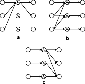

  

  a–c The normalized sum capacity of a 3×3×3 network with 1-local view, α ^∗, is equal to 1/3 if and only if one of the graphs in this figure is a subgraph of $\mathcal {G}$

• 3. 1/2 otherwise.

As we show in this section, the transmission strategy is a combination of three main techniques:

• 1. Per layer interference avoidance

• 2. Repetition coding to allow overhearing of the interference

• 3. Network coding to allow interference neutralization

Remark 6

From Theorems 3 and 4, we conclude that for all single-layer, K×2×K, and 3×3×3 networks with 1-local view, the normalized sum capacity α ^∗=1/K (i.e., TDMA) is optimal if and only if when all channel gains are equal and non-zero, then there exists a node that can decode all messages. We refer to such node as an “omniscient” node. We believe this observation holds for much more general network connectivities with 1-local view or in fading networks with no channel state information at the transmitters. However, this is a different line of research and it is beyond the scope of this paper. Omniscient nodes are studied in [ 29 , 30 ] in the context of two-source two-destination multi-layer wireless networks where they dictate the asymptotic (in terms of power) behavior of these networks.

Proof

Achievability: The achievability proof for networks in category (a) is trivial as there is no interference present in such networks. For networks in category (b), a simple TDMA achieves a normalized sum rate of 1/3. Thus, we only need to prove the result for networks in category (c).

Suppose none of the graphs in Fig. 11 is a subgraph of $\mathcal {G}$ and that the network does not fall in category (a). This immediately implies d _max=2.

We have the following claim for such networks.

Claim 1

For a 3×3×3 network with d _max=2, the only connectivity that results in a per layer fully connected conflict graph is the one shown in Fig. 12.

Fig. 12

The only connectivity that results in a per layer fully connected conflict graph in a 3×3×3 network with d _max=2

If the per layer conflict graphs are not fully connected and the network does not fall in category (a), then a normalized sum rate of α=1/2 is easily achievable. Moreover, from claim 1, we know that with d _max=2, the folded-chain structure of Fig. 12 exists in at least one of the layers. In Section 3, we showed that a normalized sum rate of α=1/2 is achievable.

We note that these cases can be easily described within the algebraic framework of Section 4. In fact, if the folded-chain structure of Fig. 12 exists in at least one of the layers, as shown in Section 3, the transmission can be expressed as a valid assignment of transmit and receive matrices. However, if the per layer conflict graphs are not fully connected and the network does not fall in category (a), then the scheme is a per layer interference avoidance which can be easily expressed in terms of a valid assignment of transmit and receive matrices. Finally, we note that for all 3×3×3 networks, the assignment of the transmit vectors and matrices is the same for the linear deterministic model and the Gaussian model.

Converse: The forward direction of the proof for networks in category (a) is trivial as there is no interference present in such networks. For the reverse direction as shown in Lemma 3 Appendix A, for any network that does not fall into category (a), an upper bound of 1/2 on the normalized sum capacity holds. Moreover, Lemma 3 also provides the outer-bound for networks in category (c). Thus, we only need to consider 3×3×3 networks in category (b).

For 3×3×3 networks in category (b), we first consider the forward direction. One of the graphs in Fig. 11 is a subgraph of the network connectivity graph $\mathcal {G}$, say the graph in Fig. 11b. Assign channel gain of $n \in \mathbb {N}$ (in linear deterministic model) and $h \in \mathbb {C}$ (in Gaussian model) to the links of the subgraph and channel gain of 0 to the links that are not in the graph of Fig. 11b.

With this assignment of the channel gains, we have

$$\begin{array}{*{20}l} H\left(W_{i} | Y_{\mathsf{A}_{i}}^{n}, L_{\mathsf{A}_{i}}, \mathsf{SI} \right) \leq n \epsilon_{n}, \qquad i=1,2,3. \end{array} $$

(51)

Basically, each destination D _i is only connected to relay A _i , and each relay A _i has all the information that destination D _i requires in order to decode its message, i=1,2,3. Thus, relay A ₁ can decode W₁. After removing the contribution of S ₁, relay A ₁ is able to decode W₂. Continuing this argument, we conclude that

$$\begin{array}{*{20}l} n \left(\sum_{j=1}^{3}{R_{j}} - \epsilon_{n} \right) \leq H\left(Y_{\mathsf{A}_{1}}^{n} | L_{\mathsf{A}_{1}}, \mathsf{SI} \right). \end{array} $$

(52)

$$ {{}\begin{aligned} &\mathbf{R}_{\mathsf{D}_{1}} =\\ &\qquad\qquad\mathsf{S}_{1}:\mathsf{V}_{1}\quad\quad\mathsf{S}_{2}:\mathsf{V}_{4} \quad\quad\mathsf{S}_{3}:\mathsf{V}_{4} \quad\quad\mathsf{S}_{3}:\mathsf{V}_{5} \quad\quad\mathsf{S}_{4}:\mathsf{V}_{1} \quad\quad\mathsf{S}_{4}:\mathsf{V}_{4}\quad\quad\mathsf{S}_{4}:\mathsf{V}_{5}\quad\quad\mathsf{S}_{5}:\mathsf{V}_{1} \quad\quad\mathsf{S}_{5}:\mathsf{V}_{5}\\ &\begin{array}{c} t= 1\\ t = 2\\ t = 2 \end{array} \left(\!\!\! \begin{array}{ccccccccc} {\phantom{000}}1 {\phantom{000}}& {\phantom{0000}}1 {\phantom{0000}}& {\phantom{0000}}0 {\phantom{000}}& {\phantom{0000}}1 {\phantom{0000}}& {\phantom{0000}}0 {\phantom{0000}}& {\phantom{000}}1 {\phantom{0000}}& {\phantom{0000}}1 {\phantom{0000}}& {\phantom{0000}}0 {\phantom{000}}& {\phantom{0000}}1{\phantom{0000}}\\ 1 & 1 & 0 & 1 & 1 & 0 & 0 & 0 & 1\\ 1 & 0 & 1 & 1 & 1 & 0 & 0 & 1 & 0 \\ \end{array}\!\!\! \right), \end{aligned}} $$

(53)

The MAC capacity at relay A ₁, for the linear deterministic model, gives us

$$ 3 (\alpha n - \tau) \leq n \Rightarrow (3 \alpha - 1) n \leq d \tau. $$

(53)

Since this has to hold for all values of n, and α and τ are independent of n, we get $\alpha \leq \frac {1}{3}$. For the Gaussian model, the MAC capacity at relay A ₁ gives us

$$ 3 (\alpha \log(1+|h|^{2}) - \tau) \leq \log(1+ 3 \times |h|^{2}), $$

(54)

which results in

$$ (3 \alpha - 1) \log(1+|h|^{2}) \leq \log(3) + 3 \tau. $$

(55)

Since this has to hold for all values of h, and α and τ are independent of h, we get $\alpha \leq \frac {1}{3}$. The proof for the graphs in Fig. 11a, c is very similar.

For the reverse direction, if none of the graphs in Fig. 11 is a subgraph of the network connectivity graph $\mathcal {G}$, a normalized sum rate of $\alpha = \frac {1}{2}$ is achievable and optimal. This completes the converse proof.

5.4 Folded-chain networks

We now consider a class of networks for which we need to incorporate network coding in order to achieve the normalized sum capacity with 1-local view. This class is the generalization of the networks in Section 5.1 to two layers.

Definition 9

A two-layer (K,m) folded-chain network (1≤m≤K) is a two-layer network with K S-D pairs and K relays in the middle. Each S-D pair i has m disjoint paths, through relays with indices 1+[{(i−1)⁺+(j−1)}m o d K] where i=1,…,K, j=1,…,m.

Theorem 5

The normalized sum capacity of a two-layer (K,m) folded-chain network with 1-local view is $\alpha ^{\ast } = \frac {1}{m}$.

Proof

Achievability: The result is trivial for m=1. For m=K, the upper bound of $\alpha = \frac {1}{K}$ can be achieved simply by using TDMA. Similar to Theorem 2, suppose m<K<2m. The extension to the general case would be similar to Theorem 2. Here, we describe how to construct a valid assignment of transmit and receive matrices.

The assignment of the transmit vectors in the first layer is identical to that of Theorem 2 as given in (35). We note that each relay can recover all incoming signals with this assignment. For the second layer, we have K+1 steps.

∙ Steps 1 through m: Our goal is to provide destination D _i , 1≤i≤m, during time slot i with its desired signal without any interference. Therefore, row i of any relay connected to D _i has a single 1 in the column associated with S-D pair i and 0s elsewhere;

∙ Steps m+1 through K: During step i, m+1≤i≤K, our goal is to provide destination D _i with its desired signal (interference will be handled later). To do so, consider the transmit matrix of any relay connected to s f D _i ; and place a single 1 in the column associated with S-D pair i and the row with the smallest index and least number of 1s;

∙ Step K+1: During this step, our goal is to resolve interference and goes through the following loop:

• 1. Let $\mathcal {L}_{j}$ denote the set of row indices for which there exists at least 1 in the column associated with S-D pair j of the transmit matrix of a relay connected to D _j , m+1≤j≤K;

• 2. Set j=m+1. For any j ^′≠j, j ^′=1,2,…,K, if

  $$\begin{array}{*{20}l} \sum_{p: \mathsf{V}_{p} \text{~connected~to~} \mathsf{D}_{j}}\sum_{\ell \in \mathcal{L}_{j}} \mathbf{T}_{\mathsf{V}_{p}}\left(\ell, \mathsf{ S}_{j^{\prime}} \right) \neq 0, \end{array} $$

  (57)

  then make this summation 0 making any of the $\mathbf {T}_{\mathsf {V}_{p}}\left (\ell, \mathsf {S}_{j^{\prime }} \right)$’s that is not previously assigned equal to 1⁴;

• 3. Set j=j+1; If j>K and during the previous loop no change has occurred, then set all entries that are not yet defined equal to zero and terminate; otherwise, go to line 2 of the loop.

We now describe the K+1 steps via an example of (5,3) two-layer folded-chain network of Fig. 13. In Fig. 14, we have demonstrated the evolution of the relays’ transmit matrices at the end of steps m, K, and K+1. For this example, the loop in step K+1 is repeated three times.

Fig. 13

A (5,3) two-layer folded-chain network

Fig. 14

The evolution of the relays’ transmit matrices at the end of steps m, K, and K+1. For this example, the loop in step K+1 is repeated three times

It is easy to verify condition C.3 for destination D ₁, D ₂, and D ₃. We have provided $\mathbf {R}_{\mathsf {D}_{4}}\phantom {\dot {i}\!}$ in (53), and as we can see, by adding the first and the second row, we can have a row that has only 1s in the columns corresponding to source S ₄. Similarly, we can show that the condition holds for D ₅.

Converse: Assume that a normalized sum rate of α is achievable, i.e., there exists a transmission strategy with 1-local view, such that for all channel realizations, it achieves a sum rate satisfying

$$\begin{array}{*{20}l} \sum_{i=1}^{K}{R_{i}} \ge \alpha C_{\text{sum}} -\tau, \end{array} $$

(58)

with error probabilities going to zero as N→∞ and for some constant τ∈R independent of the channel gains.

Consider the first layer of the two-layer (K,m) folded-chain network, where the channel gain of a link from source i to relays i,i+1,…,m is equal to $n \in \mathbb {N}$ (for the linear deterministic model) and $h \in \mathbb {C}$ (for the Gaussian model), i=1,2,…,m, and all the other channel gains are equal to zero. In the second layer, we set the channel gain from relay i to destination i equal to n (for the linear deterministic model) or h (for the Gaussian model), and all other channel gains equal to 0, i=1,2,…,m. See Fig. 15 for a depiction.

Fig. 15

Channel gain assignment in a two-layer (K,m) folded-chain network. All solid links have capacity n (for the linear deterministic model) and h (for the Gaussian model), and all dashed links have capacity 0

With this configuration, each destination D _i is only connected to relay A _i , and each relay A _i has all the information that destination D _i requires in order to decode its message, i=1,…,m. We have

$$\begin{array}{*{20}l} H\left(W_{i} | Y_{\mathsf{A}_{i}}^{n}, L_{\mathsf{A}_{i}}, \mathsf{SI} \right) \leq n \epsilon_{n}, \qquad i=1,\ldots,m. \end{array} $$

(59)

At relay A _m after decoding and removing the contribution of S _m , relay A _m is able to decode W _m−1. With a recursive argument, we conclude that

$$\begin{array}{*{20}l} n \left(\sum\limits_{j=1,2,\ldots,m}{R_{j}} - \epsilon_{n} \right) \leq H\left(Y_{\mathsf{A}_{m}}^{n} | L_{\mathsf{A}_{m}}, \mathsf{SI} \right). \end{array} $$

(60)

The MAC capacity at relay A _m for the linear deterministic model gives us

$$ m (\alpha n - \tau) \leq n \Rightarrow (m \alpha - 1) n \leq d \tau. $$

(61)

Since this has to hold for all values of n, and α and τ are independent of n, we get $\alpha \leq \frac {1}{m}$. For the Gaussian model, the MAC capacity at relay A _m gives us

$$ m (\alpha \log(1+|h|^{2}) - \tau) \leq \log(1+ m \times |h|^{2}), $$

(62)

which results in

$$ (m \alpha - 1) \log(1+|h|^{2}) \leq \log(m) + m \tau. $$

(63)

Since this has to hold for all values of h, and α and τ are independent of h, we get $\alpha \leq \frac {1}{m}$. □

5.5 Gain of coding over interference avoidance: nested folded-chain networks

In this subsection, we show that the gain from using coding over interference avoidance techniques can be unbounded. To do so, we first define the following class of networks.

Definition 10

An L-nested folded-chain network is a single-layer network with K=3^L S-D pairs, $\phantom {\dot {i}\!}\{ \mathsf {S}_{1}, \ldots, \mathsf { S}_{3^{L}} \}$ and $\phantom {\dot {i}\!}\{ \mathsf {D}_{1}, \ldots, \mathsf {D}_{3^{L}} \}$. For L=1, an L-nested folded-chain network is the same as a single-layer (3,2) folded-chain network. For L>1, an L-nested folded-chain network is formed by first creating three copies of an (L−1)-nested folded-chain network. Then,

• The i-th source in the first copy is connected to the i-th destination in the second copy, i=1,…,3^L−1,

• The i-th source in the second copy is connected to the i-th destination in the third copy, i=1,…,3^L−1,

• The i-th source in the third copy is connected to the i-th destination in the first copy, i=1,…,3^L−1.

Figure 16 illustrates a 2-nested folded-chain network.

Fig. 16

A 2-nested folded-chain network

Consider an L-nested folded-chain network. The conflict graph of this network is fully connected, and as a result, interference avoidance techniques can only achieve a normalized sum rate of $\left (\frac {1}{3} \right)^{L}$. However, we know that for a single-layer (3,2) folded-chain network, a normalized sum rate of $\frac {1}{2}$ is achievable.

Hence, applying our scheme to an L-nested folded-chain network, a normalized sum rate of $\left (\frac {1}{2} \right)^{L}$ is achievable. For instance, consider the 2-nested folded-chain network in Fig. 16. We show that any transmission strategy over the induced subgraphs can be implemented in the original network by using only four time slots such that all nodes receive the same signal as if they were in the induced subgraphs.

To achieve a normalized sum rate of $\alpha = \left (\frac {1}{2} \right)^{2}$, we split the communication block into four time slots of equal length. During time slot 1, sources 1, 2, 4, and 5 transmit the same codewords as if they are in the induced subgraphs. During time slot 2, sources 3 and 6 transmit the same codewords as if they are in the induced subgraphs, and sources 2 and 5 repeat their transmit signal from the first time slot. During time slot 3, sources 7 and 8 transmit the same codewords as if they are in the induced subgraphs, and sources 4 and 5 repeat their transmit signal from the first time slot. During time slot 4, source 9 transmits the same codewords as if it is in the induced subgraph, and sources 5, 6, and 8 repeat their transmit signal.

It is straightforward to verify that with this scheme, all destinations receive the same signal as if they were in the induced subgraphs. Hence, a normalized sum rate of $\alpha = \left (\frac {1}{2} \right)^{2}$ is achievable for the network in Fig. 16. Therefore, the gain of using coding over interference avoidance is $\left (\frac {3}{2} \right)^{L}$ which goes to infinity as L→∞. See Fig.17 for a depiction. As a result, we can state the following lemma.

Fig. 17

a Achievable normalized sum rate of coding and interference avoidance in an L-nested folded-chain network and b the performance gain of coding scheme over interference avoidance

Lemma 2

Consider an L-nested folded-chain network. The gain of using MCL scheduling over MIL scheduling is $\left (\frac {3}{2} \right)^{L}$ which goes to infinity as L→∞.

The scheme required to achieve a normalized sum rate of $\alpha = \left (\frac {1}{2} \right)^{L}$ for an L-nested folded-chain network can be viewed as a simple extension of the results presented in Section 4. In a sense instead of reconstructing a single snapshot, we reconstruct L snapshots of the network. The following discussion is just for the completion of the results.

To each source S _i , we assign a transmit vector $\mathbf {T}_{\mathsf {S}_{i}}\phantom {\dot {i}\!}$ of size (L T)×1 where each row corresponds to a time slot. If we denote the transmit signal of node S _i in the ℓth snapshot by $X^{\ell }_{\mathsf {S}_{i}}$, then if $\mathbf {T}_{\mathsf {S}_{i}}(j) = 1\phantom {\dot {i}\!}$ and c T+1≤j<(c+1)T for c=0,1,…,L−1, then S _i communicates $X^{c+1}_{\mathsf { S}_{i}}$. The other transmit and receive matrices can be described similarly. Conditions C.2 and C.3 have to be satisfied for submatrices of $\mathbf {R}_{\mathsf {V}_{j}}\phantom {\dot {i}\!}$ corresponding to rows c T+1,c T+2,…,(c+1)T−1 for c=0,1,…,L−1.

6 Conclusions

In this paper, we studied the fundamental limits of communications over multi-layer wireless networks where each node has limited channel state information. We developed a new transmission strategy for multi-layer wireless networks with partial channel state information (i.e., 1-local view) that combines multiple ideas including interference avoidance and network coding. We established the optimality of our proposed strategy for several classes of networks in terms of achieving the normalized sum capacity. We also demonstrated several connections between network topology, normalized sum capacity, and the achievability strategies.

So far, we have only studied cases with 1-local view. One major direction is to characterize the increase in normalized sum capacity as nodes learn more and more about the channel state information. We also focused on the case in which wireless nodes know the network connectivity globally, but the actual values of the channel gains are known for a subset of flows. Another important direction would be to understand the impact of local connectivity knowledge on the capacity and to develop distributed strategies to optimally route information with partial connectivity knowledge.

7 Endnotes

¹ Since in two time slots, any transmission strategy for the diamond networks can be implemented in the original network, we can implement the strategies that achieve the capacity for any S-D pair i with full network knowledge, i.e., C _i , over two time slots as well. Hence, we can achieve $\frac {1}{2} \left (C_{1} + C_{2} + C_{3} \right)$. On the other hand, we have C _sum≤C ₁+C ₂+C ₃. As a result, we can achieve a set of rates such that $\sum _{i=1}^{3}{R_{i}} \geq \frac {1}{2} C_{\text {sum}}$, and by the definition of normalized sum rate, we achieve $\alpha = \frac {1}{2}$.

² A cut Ω is a subset of $\mathcal {V}$ such that S∈Ω,D∉Ω, and $\Omega ^{c} = \mathcal {V} \setminus \Omega$.

³ The result for m=1 is trivial since we basically have an interference-free network.

⁴ If $\mathbf {T}_{\mathsf {V}_{p}}\left (\ell, \mathsf {S}_{j^{\prime }} \right)$ is not yet assigned a 0 or 1, treat it as 0 in the summation.

8 Appendix A: Outer-bound of 1/2 for networks with interference

Lemma 3

In a K-user multi-layer network (linear deterministic or Gaussian) with 1-local view if there exists a path from S _i to D _j , for some i≠j, then the normalized sum capacity is upper-bounded by α=1/2.

Proof

Consider a path from source S _i to destination D _j , i≠j, i,j∈{1,…,K}. Assign channel gain of $n \in \mathbb {N}$ (for the linear deterministic model) and $h \in \mathbb {C}$ (for the Gaussian model) to all edges in this path. For each one of the two S-D pairs i and j, pick exactly one path from the source to the destination and assign channel gain of n (for the linear deterministic model) or h (for the Gaussian model) to all edges in these paths. Assign channel gain of 0 to all remaining edges in the network $\mathcal {G}$. See Fig. 18 for an illustration.

Fig. 18

A path exists from source S ₁ to destination D ₂; all solid edges have capacity n (for linear deterministic model) or h (for the Gaussian model) and the rest have capacity 0

In order to guarantee a normalized sum rate of α with 1-local view, each source has to transmit at a rate greater than or equal to α n−τ (for the linear deterministic model) or α log(1+|h|²)−τ (for the Gaussian model). This is due to the fact that from each source’s point of view, it is possible that the other S-D pairs have capacity 0.

Suppose this rate is feasible, i.e., destinations D _i and D _j are able to decode W _i and W _j , respectively. Since there exists a path from source S _i to destination D _j , i≠j, i,j∈{1,…,K}, we can find a node $\mathsf {V}^{\ast } \in \mathcal {V}$ such that $\mathsf {V}^{\ast } \in \mathcal {G}_{ij}$ and $\mathsf {V}^{\ast } \in \mathcal {G}_{jj}$, see Fig. 18. Node V ^∗ is able to decode W _j since it has more information than destination D _j . Node V ^∗ decodes W _j and removes it from the received signal. Now, for the Gaussian model, it has statistically the same received signal as node $\bar {\mathsf {V}}$ (a node in $\mathcal {G}_{ii}$ and in the same layer as V ^∗) and for the linear deterministic model, it has the same received signal as node $\bar {\mathsf {V}}$. Node $\bar {\mathsf {V}}$ is able to decode W _i since it has more information than destination D _i ., as a result, V ^∗ is also able to decode W _i . This means that there exists a node $\mathsf {V}^{\ast } \in \mathcal {V}$ that can decode both W _i and W _j .

Hence, the MAC capacity at V ^∗ in the linear deterministic model gives us

$$ 2 \alpha n - 2 \tau \leq n \Rightarrow (2 \alpha - 1) n \leq 2 \tau. $$

(64)

Since this has to hold for all values of n, and α and τ are independent of n, we get $\alpha \leq \frac {1}{2}$.

For the Gaussian model, the MAC capacity at V ^∗ gives us

$$ 2 (\alpha \log(1+|h|^{2}) - \tau) \leq \log(1 + 2|h|^{2}), $$

(65)

which results in

$$ (2 \alpha - 1) \log\left(1+|h|^{2}\right) \leq 1 + 2 \tau. $$

(66)

Since this has to hold for all values of h, and α and τ are independent of h, we get $\alpha \leq \frac {1}{2}$. □

9 Appendix B: Converse proof for case (2) of Theorem 3

Converse proof for case (2): If a destination is only connected to relay A ₂, assign channel gain of 0 to the link from A ₂ to such destination. Set all the other channel gains equal to $n \in \mathbb {N}$ (in the linear deterministic model) and equal to $h \in \mathbb {C}$ (in the Gaussian model). We claim that with this channel gain assignment, a destination connected to both relays should be able to decode all messages (note that with our choice of channel gains, there is no message for destinations that are only connected to relay A ₂).

Destinations that are connected to both relays receive the exact same signal (in the linear deterministic model) and the same codewords plus different noise terms (in the Gaussian model). Therefore, since each one of them is able to decode its message, then it should be able to decode the rest of the messages intended for destinations that are connected to both relays. They decode and remove such messages from the received signal. The remaining signal is the same codeword (plus different noise term in Gaussian model) received at the destinations that are only connected to relay A ₁. Therefore, those messages are also decodable at a destination that is connected to both relays.

We assume 1-local view at the sources; therefore, to achieve a normalized sum rate of α, each source should transmit at a rate greater than or equal to α n−τ (in linear deterministic model). This is due to the fact that from each source’s point of view, it is possible that the other S-D pairs have capacity 0; therefore, in order to achieve a normalized sum rate of α, it should transmit at a rate of at least α n−τ. The above argument alongside the MAC capacity at a destination connected to both relays, results in

$$ d_{\text{out}}(\mathsf{A}_{1}) (\alpha n - \tau) \leq n \Rightarrow (d_{\text{out}}(\mathsf{A}_{1}) \alpha - 1) n \leq d_{\text{out}}(\mathsf{ A}_{1}) \tau. $$

(67)

Since this has to hold for all values of n, and α and τ are independent of n, we get $\alpha \leq \frac {1}{d_{\text {out}}({ \sf A}_{1})}$.

In the Gaussian case, each source should transmit at a rate greater than or equal to α log(1+|h|²)−τ, since from each source’s point of view, it is possible that the other S-D pairs have capacity 0. Similar to the linear deterministic case, we get

$$ \begin{aligned} d_{\text{out}}(\mathsf{A}_{1}) \left(\alpha \log(1+|h|^{2}) - \tau \right) &\leq \\&\log\left(1\,+\,d_{\text{out}}(\mathsf{A}_{1}) \!\times\! |h|^{2}\right), \end{aligned} $$

(68)

or equivalently

$$ {} (d_{\text{out}}(\mathsf{A}_{1}) \alpha - 1) \log\left(1+|h|^{2}\right) \leq \log(d_{\text{out}}(\mathsf{A}_{1})) + d_{\text{out}}(\mathsf{A}_{1}) \tau. $$

(69)

Since this has to hold for all values of h, and α and τ are independent of h, we get $\alpha \leq \frac {1}{d_{\text {out}}(\mathsf {A}_{1})}$.

References

A Vahid, V Aggarwal, AS Avestimehr, A Sabharwal, in 48th Annual Allerton Conference on Communication, Control, and Computing. On the capacity of multi-hop wireless networks with partial network knowledge (IEEEAllerton Park, Monticello, 2010), pp. 1030–1037.
V Aggarwal, AS Avestimehr, A Sabharwal, On achieving local view capacity via maximal independent graph scheduling. IEEE Trans. Inf. Theory. 57(5), 2711–2729 (2011).
SA Jafar, Topological interference management through index coding. IEEE Trans. Inf. Theory. 60(1), 529–568 (2014).
H Maleki, VR Cadambe, SA Jafar, Index coding—an interference alignment perspective. IEEE Trans. Inf. Theory. 60(9), 5402–5432 (2014).
M Ji, G Caire, AF Molisch, Fundamental limits of caching in wireless D2D networks. IEEE Trans. Inf. Theory. 62(2), 849–869 (2016).
N Naderializadeh, AS Avestimehr, Interference networks with no CSIT: impact of topology. IEEE Trans. Inf. Theory. 61(2), 917–938 (2015).
H Sun, C Geng, SA Jafar, in IEEE International Symposium on Information Theory Proceedings (ISIT). Topological interference management with alternating connectivity (IEEEIstanbul, 2013), pp. 399–403.
X Yi, D Gesbert, Topological interference management with transmitter cooperation. IEEE Trans. Inf. Theory. 61(11), 6107–6130 (2015).
N Naderializadeh, AS Avestimehr, ITLinQ: A new approach for spectrum sharing in device-to-device communication systems. IEEE J. Selected Areas Commun. 32(6), 1139–1151 (2014).
V Aggarwal, L Sankar, AR Calderbank, HV Poor. Ergodic layered erasure one-sided interference channels (IEEETaormina, 2009), pp. 574–578.
C Wang, T Gou, SA Jafar, Aiming perfectly in the dark-blind interference alignment through staggered antenna switching. IEEE Trans. Signal Process. 59(6), 2734–2744 (2011).
SA Jafar, in IEEE Global Telecommunications Conference (GLOBECOM 2010). Exploiting channel correlations-simple interference alignment schemes with no CSIT (IEEEMiami, 2010), pp. 1–5.
A Vahid, MA Maddah-Ali, AS Avestimehr, Y Zhu, Binary fading interference channel with no CSIT. IEEE Trans. Inf. Theory. 63(6), 3565–3578 (2017).
H Maleki, SA Jafar, S Shamai, Retrospective interference alignment over interference networks. IEEE J. Selected Topics Signal Process. 6(3), 228–240 (2012).
CS Vaze, MK Varanasi, The degrees of freedom region and interference alignment for the MIMO interference channel with delayed CSIT. IEEE Trans. Inf. Theory. 58(7), 4396–4417 (2012).
A Vahid, MA Maddah-Ali, AS Avestimehr, Capacity results for binary fading interference channels with delayed CSIT. IEEE Trans. Inf. Theory. 60(10), 6093–6130 (2014).
MA Maddah-Ali, D Tse, Completely stale transmitter channel state information is still very useful. IEEE Trans. Inf. Theory. 58(7), 4418–4431 (2012).
A Vahid, MA Maddah-Ali, AS Avestimehr, Approximate capacity region of the MISO broadcast channels with delayed CSIT. IEEE Trans. Commun. 64(7), 2913–2924 (2016).
A Vahid, MA Maddah-Ali, AS Avestimehr, Communication through collisions: opportunistic utilization of past receptions (IEEE International Conference on Computer Communications (INFOCOM), Toronto, 2014).
A Vahid, R Calderbank, in 2015 IEEE International Symposium on Information Theory (ISIT). Impact of local delayed CSIT on the capacity region of the two-user interference channel (IEEEHong Kong, 2015), pp. 2421–2425.
A Vahid, R Calderbank, in 2016 IEEE International Symposium on Information Theory (ISIT). When does spatial correlation add value to delayed channel state information? (IEEEBarcelona, 2016), pp. 2624–2628.
A Vahid, R Calderbank, Two-user erasure interference channels with local delayed CSIT. IEEE Trans. Inf. Theory. 62(9), 4910–4923 (2016).
OE Ayach, RW Heath Jr, Interference alignment with analog channel state feedback. IEEE Transactions on Wireless Communications. 11(2), 626–636 (2012).
V Aggarwal, Y Liu, A Sabharwal, in Proceedings of International Symposium on Information Theory (ISIT). Message passing in distributed wireless networks (IEEESeoul, 2009), pp. 1090–1094.
V Aggarwal, Y Liu, A Sabharwal, Sum capacity of interference channels with a local view: impact of distributed decisions. IEEE Trans. Inf. Theory. 58(3), 1630–1659 (2012).
D Blackwell, L Breiman, AJ Thomasian, The capacity of a class of channels. Ann. Math. Stat. 30:, 1229–1241 (1959).
A Raja, VM Prabhakaran, P Viswanath, The two user Gaussian compound interference channel. IEEE Trans. Inf. Theory. 55(11), 5100–5120 (2009).
AS Avestimehr, S Diggavi, D Tse, Wireless network information flow: a deterministic approach. IEEE Trans. Inf. Theory. 57(4), 1872–1905 (2011).
I Shomorony, AS Avestimehr, Two-unicast wireless networks: characterizing the degrees of freedom. IEEE Trans. Inf. Theory. 59(1), 353–383 (2013).
A Vahid, I Shomorony, R Calderbank, in 53rd Annual Allerton Conference on Communication, Control, and Computing. Informational bottlenecks in two-unicast wireless networks with delayed CSIT (IEEEAllerton Park, Monticello, 2015), pp. 1256–1263.
Acknowledgements
The authors would like to thank Kanes Sutuntivorakoon of Rice University for helpful discussions related to Section V. C of this paper.
Funding
The work of A. Vahid is in part supported by Qualcomm Innovation Fellowship. The work of A. S. Avestimehr is in part supported by NSF grant CCF-1419632 and ONR award N000141612189.
Author information
Authors and Affiliations
Contributions
This work was done by AV as part of his PhD studies. He was advised by Professors VA, ASA, and AS. All authors read and approved the final manuscript.
Corresponding author
Ethics declarations
Competing interests
The authors declare that they have no competing interests.
Publisher’s Note
Springer Nature remains neutral with regard to jurisdictional claims in published maps and institutional affiliations.
Rights and permissions
Open Access This article is distributed under the terms of the Creative Commons Attribution 4.0 International License (http://creativecommons.org/licenses/by/4.0/), which permits unrestricted use, distribution, and reproduction in any medium, provided you give appropriate credit to the original author(s) and the source, provide a link to the Creative Commons license, and indicate if changes were made.
About this article
Cite this article
Vahid, A., Aggarwal, V., Avestimehr, A. et al. Interference management with mismatched partial channel state information. J Wireless Com Network 2017, 134 (2017). https://doi.org/10.1186/s13638-017-0917-0
Received:
Accepted:
Published:
DOI: https://doi.org/10.1186/s13638-017-0917-0