Cross-layer link adaptation for goodput optimization in MIMO BIC-OFDM systems

Abstract

This work proposes a novel cross-layer link performance prediction (LPP) model and link adaptation (LA) strategy for soft-decoded multiple-input multiple-output (MIMO) bit-interleaved coded orthogonal frequency division multiplexing (BIC-OFDM) systems employing hybrid automatic repeat request (HARQ) protocols. The derived LPP, exploiting the concept of effective signal-to-noise ratio mapping (ESM) to model system performance over frequency-selective channels, does not only account for the actual channel state information at the transmitter and the adoption of practical modulation and coding schemes (MCSs), but also for the effect of the HARQ mechanism with bit-level combining at the receiver. Such method, named aggregated ESM, or αESM for short, exhibits an accurate performance prediction combined with a closed-form solution, enabling a flexible LA strategy, that selects at every protocol round the MCS maximizing the expected goodput (EGP), i.e., the number of correctly received bits per unit of time. The analytical expression of the EGP is derived capitalizing on the αESM and resorting to the renewal theory. Simulation results carried out in realistic wireless scenarios corroborate our theoretical claims and show the performance gain obtained by the proposed αESM-based LA strategy when compared with the best LA algorithms proposed so far for the same kind of systems.

1 Introduction

To meet the demanding need for ever increasing data rate and reliability, orthogonal frequency division multiplexing (OFDM), bit-interleaved coded modulation (BICM) [2], spatial multiplexing (SM) via multiple-input multiple-output (MIMO) [3], adaptive modulation and coding (AMC) [4], and hybrid automatic repeat request (HARQ) [5] are well-known techniques currently adopted, as advanced LTE (LTE-A) [6], and envisaged to be exploited in the future wireless systems [7]. To be specific, the HARQ technique combines the automatic repeat request (ARQ) mechanism with both the channel coding error correction and the error detection capability of the cyclic redundancy check (CRC) [5]. If the CRC is successfully detected, the packet is correctly received and an acknowledgement (ACK) is fed back to the transmitter. Conversely, a CRC failure means that the received packet is affected by uncorrected errors and a non-ACK (NACK) is sent back. In the latter condition, a retransmission of the corrupted packet is performed according to one of the following HARQ strategies [8]: (i) type I or Chase Combining (CC), the packet is retransmitted using the same redundancy; (ii) type II with partial Incremental Redundancy (IR), only a subset of previously unsent redundancy is transmitted; and (iii) type II with full IR, the systematic bits plus a different set of coded bits than those previously transmitted are sent. The HARQ mechanism potentials are fully exploited when the receiver suitably combines, e.g., using maximum ratio combining (MRC), the currently retransmitted packet with the previously unsuccessfully received ones, thus building a single packet whose reliability is more and more increased [5]. HARQ combining can be performed either on the received symbols or, should a different symbol mapping be employed in each transmission round, at bit-level, i.e., by accumulating the bit log-likelihood ratio (LLR) metrics [9].

Background and related works. In the literature, a considerable effort has been put in quantifying the performance limits for HARQ-based transmissions, mainly focusing on the ergodic capacity and outage probability [10–12]. In [10], an information-theoretical study about the throughput of HARQ signaling schemes is given for the Gaussian collision channel. Then, starting from [10, 11] presents a mutual information (MI) based analysis of the long-term average transmitted rate achieved by HARQ in a block-fading scenario, which allows to adjust the rate so that a target outage probability is not exceeded. In [12], the optimal tradeoff among throughput, diversity gain, and delay is derived for an ARQ block-fading MIMO channel with discrete signal constellations.

In order to further enhance the system performance, the HARQ approach can be made adaptive by applying link adaptation (LA) strategies that do not only account for the information coming not only from the physical layer, but also from the higher layer schemes based on packet combining, so obtaining a cross-layer optimization of the link resource utilization. Most of the works considering such an issue, however, focus on theoretical performance limits based on capacity and channel outage probability, as in [13–17]. Specifically, [13] investigates the problem of power allocation for rate maximization under quantized channel state information (CSI) feedback, [14] adapts the transmission rates using the outdated CSI, whereas [15] proposes two power allocation schemes: one minimizes the transmitted power under a given packet drop rate constraint and the other minimizes the packet drop rate under the available power constraint. Note that in [13–15], IR HARQ is considered to optimize performance under narrowband fading channels. In [16], user and power are jointly selected in a multi-user contest under slow-fading channels and outdated CSI to maximize system goodput (GP), whereas [17] proposes a user, rate, and power allocation policy for GP optimization in multi-user OFDM systems with ACK-NACK feedback.

Only few recent works, however, consider practical modulation and coding schemes (MCSs). In [18], the outlined AMC algorithm maximizes the spectral efficiency under truncated HARQ for narrowband fading channels. A power minimization problem under individual user GP constraint is tackled in [19] for an orthogonal frequency division multiple access (OFDMA) network employing type II HARQ and only statistical knowledge of CSI. The work in [20] proposes the selection of the MCS to maximize GP performance in MIMO-OFDM systems under CC HARQ, where the packet error rate is evaluated through the exponential effective SNR mapping (ESM) method (EESNR). A similar approach is proposed in [21], although the physical layer performance is modeled using the MI based effective SNR (MIESM).

Rationale and contributions. In this paper, we propose a novel cross-layer link performance prediction (LPP) methodology for packet-oriented MIMO bit-interleaved coded (BIC)-OFDM transmissions which accounts for (i) practical MCSs, (ii) the HARQ mechanism with bit-level combining at the receiver, and (iii) the CSI information at the transmitter. The method allows the derivation of an LA strategy which is capable of selecting the MCS that maximizes the number of information bits correctly received per unit of time, or GP for short, at the user equipment (UE). The main features of the proposed method and the relevant improvements compared with the literature are outlined as follows.

• 1. The proposed LPP model, named aggregated ESM, or αESM, relies on the ESM concept [22], which enables the prediction of the performance of a multicarrier system affected by frequency-selective fading by compressing all the per-subchannel (identified by the pair subcarrier and spatial stream) SNRs into a scalar value representing the SNR of a coded equivalent binary system working over additive white Gaussian noise (AWGN) channel.

  • The LPP we put forward exhibits an accurate performance prediction combined with a closed-form solution which makes it eligible for practical implementation of LA algorithms. Indeed, at the generic protocol round (PR) ℓ of a given packet, the αESM is obtained recursively, by combining the aggregated effective SNR (ESNR), that stores the performance up to the previous retransmission (step ℓ−1), with the actual ESNR at PR ℓ, which depends on the current CSI and choice of the MCS.

• 2. The proposed αESM is derived from the ESM method originally proposed in [23] as κESM, by taking into account the per-subchannel SNRs along with the HARQ mechanism. The key idea of the αESM method is to properly combine together the bit LLR metrics relevant to the retransmissions of the same packet, with the result of increasing decoding reliability. Specifically, the combined bit LLR metrics are characterized following an accurate method based on the cumulant moment generating function (CMGF).

  • The αESM is shown to overcome the limitations exhibited by [20, 21], where the MCS used in the subsequent retransmission is identical with that originally chosen, in that the LPP works with CC only. Conversely, since the proposed method has the inherent possibility of choosing the MCS optimizing the GP metric within the retransmissions of the same packet, as a result, it enables a much more flexible LA strategy.

• 3. The formulation of the GP at the transmitter, named expected goodput (EGP), is derived resorting to the renewal theory framework [24] and the long-term channel static assumption [20, 21]. The goal is, indeed, to obtain a reliable performance metric that can lead to a manageable LA optimization problem. Towards this end, both theoretical and numerical analyses are employed throughout the paper to corroborate our claims and findings.

• 4. Finally, simulation results carried out over realistic wireless channels testify the advantages obtained employing the proposed LA strategy based on the αESM, when compared with the best algorithms known so far.

Organization. The rest of the paper is organized as follows. Section 2 describes the HARQ retransmission mechanism and the MIMO BIC-OFDM system. In Section 3, after a brief rationale and review of the κESM LPP, the proposed αESM model is derived. Section 4 derives the EGP formulation and describes the proposed GP-oriented (GO) LA strategy. Finally, Section 5 illustrates the numerical results, whereas in Section 6, a few conclusions are drawn.

Notations. Matrices are in uppercase bold, column vectors are in lowercase bold, [·]^T is the transpose of a matrix or a vector, a_i,j represents the entry (i,j) of the matrix A, × is the Cartesian product, calligraphic symbols, e.g., ${\mathcal {A}}$, represent sets, $|{\mathcal {A}}|$ is the cardinality of ${\mathcal {A}}$, ${\mathcal {A}}(i)$ is the ith element of ${\mathcal {A}}$, ⌈·⌉ denotes the ceil function, and E _x {·} is the statistical expectation with respect to (w.r.t.) the random variable (RV) x.

2 System model

In this section, we first describe the HARQ retransmission protocol. Then, the MIMO BIC-OFDM signalling system is outlined.

2.1 HARQ retransmission protocol

In order to enable reliable and spectral efficient packet transmissions, a HARQ retransmission protocol, with a maximum of L rounds, is jointly designed along with an AMC mechanism. The information to be transmitted is conveyed by packets (typically IP packets) received from the upper layers of the stack, i.e., layer 3 and above, and stored in an infinite-length buffer at the data link layer. At the radio link control (RLC) sublayer, each packet is mapped into a RLC protocol data unit (PDU) made of the three sections: (i) header, with size N_h; (ii) payload, with size N_p; and (iii) CRC for error detection, with size N_CRC. As shown in Fig. 1, at the generic PR $\ell \in \mathcal {L}_{\text {PR}} \triangleq \{1,\cdots,L\}$, the RLC-PDU is encoded with a code rate $r^{(\ell)}\in \mathcal {D}_{r} \triangleq \{r_{0}, r_{1}, \cdots, r_{\text {max}}\}$, thus producing $N^{(\ell)}_{\mathrm {c}}\triangleq N_{\mathrm {s}}/r^{(\ell)}\le {\bar N}_{c}$ coded binary symbols, or coded bits for short, where $N_{\mathrm {s}} \triangleq N_{\mathrm {h}}+N_{\mathrm {p}}+N_{\text {CRC}}$ and ${\bar N}_{c} \triangleq N_{\mathrm {s}}/r_{0}$, which is the number of coded bits at the output of the mother code, i.e., prior to puncturing. The $N^{(\ell)}_{\mathrm {c}}$ coded bits are transmitted using the MIMO BIC-OFDM system described in Section 2.2 over the available band W.

Fig. 1

Equivalent block scheme of the MIMO BIC-OFDM system

After the transmission of each packet¹, the receiver sends back a 1-bit feedback about the successful (ACK) or unsuccessful (NACK) packet reception. Whenever a NACK is received, the transmitter sends again the packet by encoding it with either the same puncturing pattern, a different subset of redundancy bits, or a tradeoff, according to the type of HARQ. This goes on until the transmitter receives an ACK or the maximum number of retransmissions L is reached. For both cases, the packet is removed from the buffer and the transmitter moves on sending the subsequent ones. At the receiver side, according to the HARQ scheme, for a given packet, the previously unsuccessfully received copies are stored and combined with the new received ones, thus creating more reliable metrics [5]. Since at each PR a different symbol mapping per subchannel may be applied, it is not possible to pre-combine received symbols. Hence, the packet combining strategy consists of accumulating the bit LLR metrics [9], as explained in detail in the following sections.

2.2 MIMO BIC-OFDM system

At the PR $\ell \in {\mathcal {L}}_{\text {PR}}$, the $N_{\mathrm {c}}^{(\ell)}$ coded bits are randomly interleaved and mapped onto the physical resources available in the space-time-frequency grid of the MIMO BIC-OFDM system, whose equivalent block scheme is depicted in Fig. 1. Specifically, we consider a MIMO BIC-OFDM system with N available subcarriers, N _T transmit and N _R receive antennas, employing SM and uniform power allocation across the subchannels. We further assume a block-fading channel model and spatially uncorrelated antennas. Moreover, denoting with $\mathbf {H}^{(\ell)}_{n} \in {\mathbb {C}}^{N_{R}\times N_{T}}$, the channel matrix over the nth subcarrier, $n \in \mathcal {N} \triangleq \{1,\cdots,N\}$, whose generic entry in position (ν₁,ν₂) is denoted by $h^{(\ell)}_{n,\nu _{1},\nu _{2}}$, ν₁=1,⋯,N _R , ν₂=1,⋯,N _T , we recall that SM relies on the singular value decomposition [25]

$$ \mathbf{H}^{(\ell)}_{n} = \mathbf{U}_{n}^{(\ell)}{\boldsymbol{\Theta}}_{n}^{(\ell)}{\mathbf{V}_{n}^{(\ell)}}^{*}, $$

(1)

where $\mathbf {U}_{n}^{(\ell)} \in {\mathbb {C}}^{N_{R} \times N_{R}}$ and $\mathbf {V}_{n}^{(\ell)} \in {\mathbb {C}}^{N_{T} \times N_{T}}$ are unitary rotation matrices and ${\boldsymbol {\Theta }}_{n}^{(\ell)} \in {\mathbb {R}}^{N_{R} \times N_{T}}$ is a rectangular matrix where the off-diagonal elements are zero, while the ordered diagonal elements are $\vartheta _{n,1}^{(\ell)}\ge \vartheta _{n,2}^{(\ell)}\ge \cdots \ge \vartheta _{n,M}^{(\ell)}\ge 0$, with $M \triangleq \min \{N_{T},N_{R}\}$. Thus, at most, the system consists of C=N·M parallel subchannels. In the following,

• we assume the CSI $\mathbf {H}^{(\ell)}_{n}$, $\forall n \in {\mathcal {N}}$, to be known at the transmitter side.

Specifically, with reference to Fig. 1, the interleaved sequence of punctured coded bits is subdivided into subsequences of $m_{n,\nu }^{(\ell)}$ bits each, which are gray-mapped onto the unit-energy symbols ${x}^{(\ell)}_{n,\nu } \in 2^{m_{n,\nu }^{(\ell)}}$-QAM constellation, i.e., one symbol per available subchannel $(n,\nu)\in {\mathcal {C}} \triangleq \{(n,\nu)|1\le n\le N, 1\le \nu \le M\}$, with $m_{n,\nu }^{(\ell)} \in {{\mathcal {D}}}_{m} = \left \{2, 4,\cdots,m_{\max } \right \}$.

Further, let us denote Φ^(ℓ)(·,·,·) as a function mapping the punctured $N_{c}^{(\ell)}$ coded bits, out of the ${\bar N}_{c}$ coded bits at the output of the mother code, into the label bits of the QAM symbols transmitted on the available subchannels, summarizing the puncturing, interleaving, and QAM mapping functions. Specifically, Φ^(ℓ)(j,n,ν)=k means that the coded bit $b^{(\ell)}_{k}$, $k\in \left \{1,\cdots,{\bar {N}}_{c}\right \}$ occupies the jth position, $j=1,\cdots,m_{n,\nu }^{(\ell)}$, within the label of the $2^{m_{n,\nu }^{(\ell)}}$-QAM symbol sent on the νth spatial stream, ν=1,⋯,M, of the nth subcarrier, n=1,⋯,N.

According to the SM approach, each sequence of QAM symbols $\mathbf {x}^{(\ell)}_{n}\triangleq \left [x^{(\ell)}_{n,1},\cdots,x^{(\ell)}_{n,{N_{T}}}\right ]^{\mathrm {T}}$ is pre-processed obtaining ${\tilde {\mathbf {x}}}^{(\ell)}_{n}\triangleq {\mathbf {V}_{n}^{(\ell)}}{\mathbf {x}}^{(\ell)}_{n}$, where ${\tilde {\mathbf {x}}}^{(\ell)}_{n}\triangleq \left [{\tilde x}^{(\ell)}_{n,1},\cdots,{\tilde x}^{(\ell)}_{n,{N_{T}}}\right ]^{\mathrm {T}}$, $\forall n \in {\mathcal {N}}$. It is worth noting that $x^{(\ell)}_{n,\nu }\triangleq 0$ for ν=M+1,⋯,N _T , if N _T >N _R , $\forall n \in \mathcal {N}$, being C subchannels available for transmission.

After that, the sequences ${\tilde {\mathbf {x}}}^{(\ell)}_{n}$, $\forall n \in {\mathcal {N}}$, are mapped onto the frequency symbols $\mathbf {y}_{\nu }^{(\ell)}\triangleq \left [{\tilde x}^{(\ell)}_{1,\nu },\cdots,{\tilde x}^{(\ell)}_{N,\nu }\right ]^{\mathrm {T}}$, for ν=1,⋯,N _T , to which conventional inverse discrete Fourier transform (DFT), parallel-to-serial conversion, and cyclic prefix (CP) insertion are applied. The resulting signal is then transmitted over a MIMO frequency-selective block-fading channel, using $N^{(\ell)}_{\text {OFDM}}\triangleq \left \lceil {N_{c}^{(\ell)}}/{\sum _{(n,\nu)\in \mathcal {C}m_{n,\nu }^{(\ell)}}} \right \rceil$ OFDM symbols.

At the receiver side, after CP removal and DFT processing at each antenna, we get

$$ {{r}}_{\nu_1}^{(\ell)} = \sum\limits_{\nu_2=1}^{N_T}{ {F}}_{\nu_1,\nu_2}^{(\ell)} {{y}}_{\nu_2}^{(\ell)} + { {w}}_{\nu_1}^{(\ell)},\;\;\;\nu_1=1,\cdots,N_R, $$

(2)

where ${\mathbf {r}}_{\nu _{1}}^{(\ell)}\triangleq \left [r_{1,\nu _{1}},\cdots,r_{N,\nu _{1}}\right ]^{\mathrm {T}}$, ${ \mathbf {F}}_{\nu _{1},\nu _{2}}^{(\ell)} \triangleq \text {diag}\left \{h^{(\ell)}_{1,\nu _{1},\nu _{2}},\right.\left.\cdots, h^{(\ell)}_{N,\nu _{1},\nu _{2}}\right \}$, ν₁=1,⋯,N _R , ν₂=1,⋯,N _T , with $h^{(\ell)}_{n,\nu _{1},\nu _{2}}$ introduced before (1), and ${\mathbf {w}}_{\nu _{1}}^{(\ell)}\triangleq \left [{ w}^{(\ell)}_{1,\nu _{1}},\cdots,\right.\left.{w}^{(\ell)}_{N,\nu _{1}}\right ]^{\mathrm {T}}$ is the thermal noise vector, whose generic entry is a zero-mean circular symmetric complex Gaussian RV with standard deviation $\sigma ^{(\ell)}_{n,\nu }$. After demultiplexing the received vectors ${\mathbf {r}}_{\nu _{1}}^{(\ell)}$, ν₁=1,⋯,N _R , ${{\tilde {\mathbf {z}}}}_{n}^{(\ell)}\triangleq \left [r_{n,1}^{(\ell)},\cdots,\right.\left.r_{n,N_{R}}^{(\ell)} \right ]^{\mathrm {T}}$, $\forall n \in {\mathcal {N}}$, are built and SM post-processing via $\mathbf {U}_{n}^{(\ell)}$, the output samples over each subcarrier are obtained as [25]

$$ \begin{aligned} &{\mathbf{z}_{n}^{(\ell)} \triangleq {\mathbf{U}_{n}^{(\ell)}}^{*} {{{\tilde{\mathbf{z}}}}_{n}^{(\ell)}} = {\boldsymbol{\Theta}}_{n}^{(\ell)} \mathbf{x}_{n}^{(\ell)} + {\boldsymbol{\varsigma}}_{n}^{(\ell)} =} \\ &=\text{diag}\left\{\vartheta_{n,1}^{(\ell)} x_{n,1}^{(\ell)} + \varsigma_{n,1}^{(\ell)},\cdots,\vartheta_{n,M}^{(\ell)} x_{n,M}^{(\ell)} + \varsigma_{n,M}^{(\ell)} \right\},\;\;\;n\in\mathcal{N}, \end{aligned} $$

(3)

where the elements of $\boldsymbol {\varsigma }_{n}^{(\ell)}\triangleq \left [{ \varsigma }^{(\ell)}_{n,1},\cdots,{\varsigma }^{(\ell)}_{n,M}\right ]^{\mathrm {T}}$ have the same distribution as those of ${ \mathbf {w}}_{\nu _{1}}^{(\ell)}$. The MIMO BIC-OFDM channel can thus be seen as a set of C parallel subchannels, represented by the diagonal matrix $\boldsymbol {\Upsilon }^{(\ell)} \triangleq \text {diag}\left \{ \boldsymbol {\Upsilon }_{1}^{(\ell)}, \cdots, \boldsymbol {\Upsilon }_{n}^{(\ell)}, \cdots, \boldsymbol {\Upsilon }_{N}^{(\ell)} \right \}$, with $\boldsymbol {\Upsilon }_{n}^{(\ell)} \triangleq \text {diag}\left \{\gamma _{n,1}^{(\ell)},\cdots,\gamma _{n,\nu }^{(\ell)},\cdots,\gamma _{n,M}^{(\ell)} \right \}$, $\forall n \in \mathcal {N}$, the generic entry $\gamma _{n,\nu }^{(\ell)}$ denoting the SNR value on subchannel (n,ν), given by

$$ \gamma_{n,\nu}^{(\ell)} \triangleq \left(\frac{\vartheta_{n,\nu}^{(\ell)}}{{\sigma_{n,\nu}^{(\ell)}}}\right)^{2}, \; \; \; \forall {(n,\nu)} \in {\mathcal{C}}. $$

(4)

Finally, the receiver evaluates the soft metrics, followed by de-interleaving and decoding.

3 Link performance prediction for HARQ-based MIMO BIC-OFDM systems

This section is organized as follows. In Section 3.1, the rationale underlying the LA strategy and LPP method is recalled. In Section 3.2, the concept of the κESM ESNR technique for MIMO BIC-OFDM systems with simple ARQ mechanism is briefly summarized. Finally, in Section 3.3, the novel LPP method, named αESM, is derived for HARQ-based MIMO BIC-OFDM systems with bit-level combining.

3.1 Rationale of the adaptive HARQ strategy

The approach to follow is to properly choose the parameters of the system described in Section 2.2, e.g., modulation order and coding rate, in order to obtain the best link performance. Such LA strategy can be formalized as a constrained optimization problem where the objective function, representing the system performance metric, is optimized over the constrained set of the available transmission parameters. Specifically, for a packet-oriented system, information-theoretical performance measure based on capacity, which relies on ideal assumptions of Gaussian inputs and infinite length codebooks, is inadequate to give an actual picture of the link performance [26]. More suitable metrics have been recently identified as the packet error rate (PER) and the GP [20, 21, 26], which in turn depends on the PER itself. Therefore, a simple yet effective link performance prediction method is required, accounting for both the CSI as well as the information coming from different techniques that further improve the transmission quality, i.e., the HARQ mechanisms with bit-level combining. In the sequel, we will focus on LPP techniques based on the well-known ESM concept, which has been shown to be the most effective framework to solve this issue, especially for multicarrier systems [22].

3.2 Background on the κESM LPP model

In multicarrier systems, where the frequency-selective channel introduces large SNR variations across the subcarriers and practical modulation and coding schemes are adopted, an exact yet manageable expression of the PER reveals to be demanding to derive. Due to these above reasons, ESM techniques are successfully employed, according to which the PER depends on the SNRs on each subcarrier through a scalar value, called ESNR. The latter represents the SNR of a single-carrier equivalent coded system working over AWGN channel, whose performance can be simply evaluated either off-line according to analytical models [27].

Within the ESM framwork, the κESM method, proposed for MIMO BIC-OFDM systems in [23], shows a remarkable tradeoff between accuracy and complexity when ARQ mechanisms are applied without any combining at the receiver. Such technique is based on the in-depth statistical characterization of the soft metrics at the input of the decoder, i.e., the bit LLR metrics $\Lambda _{k}^{(\ell)}$, which, for the kth transmitted coded bit $b_{k}^{(\ell)}$ at ℓth PR, reads as

$$ \Lambda^{(\ell)}_{k} = \log \frac { \lambda_{j}\left({b_{\Phi^{(\ell)}(j,n,\nu)}^{(\ell){\prime}}}, z^{(\ell)}_{n,\nu}\right) } { \lambda_{j}\left(b_{\Phi^{(\ell)}(j,n,\nu)}^{(\ell)}, z^{(\ell)}_{n,\nu}\right) } $$

(5)

where Φ^(ℓ)(j,n,ν)=k is the mapping function defined in Section 2.2 after (1),

$$ {{\begin{aligned} \lambda_{j}\left(a,z^{(\ell)}_{n,\nu}\right) = \sum\limits_{\tilde{x} \in {\chi_{a}}^{\left(\ell,j,n,\nu\right)}} { \exp\left(-\left|z^{(\ell)}_{n,\nu} - \sqrt{\gamma^{(\ell)}_{n,\nu}} \tilde{x} \right|^2 \right) }, \;\; a\in\left\{b_{k}^{(\ell)},{b_{k}^{(\ell)}}^{\prime}\right\}, \end{aligned}}} $$

(6)

denotes the bit decoding metric, $b_{k}^{\prime }$ is the complement of b _k , $\chi _{a}^{\left (\ell,j,n,\nu \right)}$ represents the subset of all the symbols belonging to the modulation adopted on the subchannel (n,ν), whose jth label bit is equal to a, whereas $z^{(\ell)}_{n,\nu }$ is the generic entry of the vector z^(ℓ) defined in (3) with $\gamma ^{(\ell)}_{n,\nu }$ given by (4). If coded bit $b_{k}^{(\ell)}$ is not transmitted, i.e., it is punctured at PR ℓ, note that $\Lambda ^{(\ell)}_{k}\triangleq 0$. After a few approximations, it is shown in [23] that the PER performance of the coded MIMO BIC-OFDM system over frequency-selective channel is accurately given by that of a coded BPSK system over AWGN channel having SNR equal to the κESM ESNR

$$ \gamma^{(\ell)} \triangleq - \log \left(\frac{1}{{\sum\limits_{(n,\nu)\in{\mathcal{C}}} m_{n,\nu}^{(\ell)} }} \sum\limits_{(n,\nu)\in {\mathcal{C}}} \Omega_{n,\nu}^{(\ell)}\left(m_{n,\nu}^{(\ell)}\right) \right) $$

(7)

where

$$ \Omega_{n,\nu}^{(\ell)} \left(m_{n,\nu}^{(\ell)}\right) \triangleq {\sum\limits_{\mu = 1}^{\sqrt{2^{m_{n,\nu}^{(\ell)}-2}}} {\frac{{{\psi_{m_{n,\nu}^{(\ell)}}}(\mu)}}{{{2^{{m_{n,\nu}^{(\ell)}} - 1}}}} \cdot{{\mathrm{e}}^{- \frac{{{\gamma^{(\ell)}_{n,\nu}}{{\left({\mu \cdot d_{n,\nu}^{(\min)}} \right)}^{2}}}}{4}}}} } $$

(8)

with $\psi _{m_{n,\nu }^{(\ell)}}$ and $d^{(\min)}_{n,\nu }$ being the constant values depending on the modulation order adopted on subchannel (n,ν) at PR ℓ. Expression (7) comes from the CMGF $\kappa _{\Lambda }^{(\ell)} (\hat {s})\triangleq \log \mathrm {E} \left \{ \text {e}^{\hat {s} \Lambda _{k}^{(\ell)}}\right \}$ of the bit LLR metric $\Lambda _{k}^{(\ell)}$ given by (5) evaluated at the saddlepoint $\hat {s} = 1/2$ and, specifically, ${\gamma ^{(\ell)} = - \kappa _{\Lambda }^{(\ell)} (\hat {s})}$ [23].

From (7)–(8), it has to be pointed out that γ^(ℓ) depends on the modulation order adopted on each subchannel given Γ^(ℓ).

3.3 The αESM model

In this section, we introduce the concept of aggregate ESNR mapping, or αESM for short, in order to predict the performance of the system of interest under HARQ mechanism. Specifically, by extending to the HARQ context, the method presented in [28] for the estimation of the pairwise error probability (PEP), the key idea of the αESM we will propose is built upon two concepts: (i) the decoding score, a RV whose positive tail probability yields the PEP [28], and (ii) the equivalent binary input output symmetric (BIOS) model of the BICM scheme [2] applied to the MIMO BIC-OFDM system described in Section 2.2. According to the latter, at each PR $\ell \in \mathcal {L}_{\text {PR}}$ and for each of the $N^{(\ell)}_{\text {OFDM}}$ symbols during such round, the MIMO BIC-OFDM channel is modeled as a set of

$$ B^{(\ell)}\triangleq\sum\limits_{(n,\nu)\in {\mathcal{C}}} m_{n,\nu}^{(\ell)} $$

(9)

parallel BIOS channels. We recall from Section 2.2 that $B^{(\ell)}\cdot N^{(\ell)}_{\text {OFDM}}\ge N^{(\ell)}_{c}$. From now on, for the sake of simplicity but w.l.g., we assume that only one OFDM symbol is sufficient for the transmission of the $N_{c}^{(\ell)}$-bit-long codeword, so that the dependence on the OFDM symbol index is avoided. In particular, we have $B^{(\ell)} = N_{c}^{(\ell)}$.

Considering that the exact estimation of the PER for the system at hand is a demanding problem, we will first evaluate the PEP expression, then resort to the standard union bound. The one-to-one mapping between the codeword and the associated vector of modulation symbols allows us to express the PEP as follows. Let $\mathbf {c}^{(\ell)}\triangleq \left \{c_{1}^{(\ell)},\cdots,c_{N_{c}^{(\ell)}}^{(\ell)}\right \}$ be the reference codeword (corresponding to the transmitted RLC-PDU at the ℓth PR) at the output of the puncturing device and ${\mathbf {c}^{(\ell)}}{\prime }\triangleq \left \{{c_{1}^{(\ell)}}{\prime },\cdots,{c_{N_{\mathrm {c}}^{(\ell)}}^{(\ell){\prime }}}\right \}$ the competing codeword, being $c^{(\ell)}_{i}$ the ith coded bit after puncturing. Besides, let us define Π^(ℓ)(i)=k, $i=1,\cdots,N_{c}^{(\ell)}$, $k\in \{1,\cdots,{\bar N}_{c}\}$, as the puncturing mapping such that $c^{(\ell)}_{i}=b^{(\ell)}_{\Pi ^{(\ell)}(i)}$, where $b^{(\ell)}_{\Pi ^{(\ell)}(i)}$ is the kth coded bit prior to puncturing. Then, upon denoting the reference and competing codewords as $\mathbf {b}^{(\ell)}\triangleq \left \{b_{\Pi ^{(\ell)}(1)}^{(\ell)},\cdots,b_{\Pi ^{(\ell)}\left ({N_{\mathrm {c}}^{(\ell)}}\right)}^{(\ell)}\right \}$ and ${\mathbf {b}^{(\ell)}}{\prime }\triangleq \left \{{b_{\Pi ^{(\ell)}(1)}^{(\ell){\prime }}},\cdots,{b_{\Pi ^{(\ell)}\left ({N_{\mathrm {c}}^{(\ell)}}\right)}^{(\ell){\prime }}}\right \}$, respectively, the PEP results as

$$ \text{PEP}~ \left(\mathbf{b}^{(\ell)},{\mathbf{b}^{(\ell)}}{\prime}\right) \triangleq \text{Pr} \left\{ \lambda\left({\mathbf{b}^{(\ell)}}{\prime},\mathbf{z}^{(\ell)}\right) > \lambda\left({\mathbf{b}^{(\ell)}},\mathbf{z}^{(\ell)}\right) \right\}, $$

(10)

where λ(·) is the soft decoding metric depending on the chosen decoding strategy. In the sequel, we will first recall the case where no bit combining is performed [28], and then, we will extend this approach to the bit-level combining receiver, which represents the novel contribution of the work.

No bit combining at the receiver. With reference to the equivalent BIOS model of the MIMO BIC-OFDM system as depicted in Fig. 2, the following observations hold.

• The input to the ith BIOS channel, 1≤i≤B^(ℓ), is the bit $b_{\Pi ^{(\ell)}(i)}^{(\ell)}$, which is mapped in the jth position of the label of the QAM symbol $x^{(\ell)}_{n,\nu }$ sent on subchannel (n,ν), being Φ^(ℓ)(j,n,ν)=k.

  Fig. 2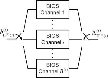

  

  Equivalent BIOS model of the MIMO BIC-OFDM system

• The output is the bit log-likelihood metric $\Lambda _{k}^{(\ell)}$, also named bit score, evaluated as in (5).

• The decoder metric for the reference codeword b^(ℓ) is the BICM maximum a posteriori metric results as [28]

  $$ \lambda ({{b}^{(\ell)}},{{z}^{(\ell)}}) = \prod\limits_{(n,\nu) \in {\mathcal{C}}} {\prod\limits_{j = 1}^{m_{n,\nu}^{(\ell)}} {\lambda_j \left({b^{(\ell)}_{\Phi^{(\ell)}(j,n,\nu)}},{z}^{(\ell)}_{n,\nu}\right)} }, $$

  (11)

  where λ _j (·,·) is the decoding metric associated to bit $b^{(\ell)}_{\Phi ^{(\ell)}(j,n,\nu)}$, evaluated according to (6), whereas that one for the competing codeword b^(ℓ)′ is obtained as in (11) by simply replacing b^(ℓ) with b^(ℓ)′.

Hence, the pairwise decoding score (PDS) relevant to the transmitted codeword b^(ℓ) with respect to b^(ℓ)′ can be written as²

$$ \Lambda_{{\text{PW}}}^{(\ell)} \triangleq \sum\limits_{(n,\nu) \in {\mathcal{C}}} {\sum\limits_{j = 1}^{m_{n,\nu}^{(\ell)}} {{\Lambda}_{\Phi^{(\ell)} (j,n,\nu)}^{(\ell)}} }, $$

(12)

where the LLR bit metric ${{\Lambda }_{\Phi ^{(\ell)} (j,n,\nu)}^{(\ell)}}$ is defined by (5). Therefore, upon plugging (11) evaluated for both b^(ℓ) and b^(ℓ)′ in the PEP expression (10), after some algebra, we obtain

$$ \text{PEP}\left(\mathbf{b}^{(\ell)},\mathbf{b}^{{(\ell)}'}\right)=\text{Pr}\left(\Lambda_{{\text{PW}}}^{(\ell)}>0 \right). $$

(13)

Bit-level combining at the receiver. The optimal receiver that accounts for the combination of all the received copies should perform a joint decoding of the pairwise decoding scores over all the possible L transmissions. However, it would result in an unfeasible complexity, exponentially increasing with L [29]. On the other side, exploiting the bit-level combining offers an effective trade-off between performance and complexity [30]. Accordingly, this is the approach we will pursue in the sequel. The decoding metric in (11) shall now account for the recombination mechanism up to the PR ℓ. At every PR indeed, the actual bit scores are evaluated as in (5) and, for each bit k, added to the bit scores evaluated during the previous PRs. Thus, the output of the equivalent BIOS channel is now the aggregate bit score

$$ {\mathcal{L}}_{k}^{(\ell)} \triangleq {{q}_{k}^{(\ell)}}^{\mathrm{T}}\boldsymbol{\Lambda}_{k}^{(\ell)}, $$

(14)

where $\boldsymbol {\Lambda }_{k}^{(\ell)} \triangleq \left [\Lambda _{k}^{(1)},\cdots,\Lambda _{k}^{(\ell)} \right ]^{\mathrm {T}}$ collects the per-round bit scores of the coded bit k up to PR ℓ and $\mathbf {q}_{k}^{(\ell)}\triangleq \left [q_{k}^{(1)},\cdots,q_{k}^{(\ell)} \right ]^{\mathrm {T}} \in \{0,1\}^{\ell }$ is the puncturing vector, that is, $q_{k}^{(i)}=1$ if bit k has been transmitted at round i, otherwise 0 if it has been punctured. In turn, the aggregate PDS at round ℓ is given by

$$ {\mathcal{L}}_{{\text{PW}}}^{(\ell)} = \sum\limits_{(n,\nu) \in {\mathcal{C}}} \sum\limits_{i=1}^{\ell} {\sum\limits_{j = 1}^{m_{n,\nu}^{(i)}} {q^{(i)}_{\Phi (j,n,\nu)} \Lambda^{(i)}_{\Phi (j,n,\nu)}} }. $$

(15)

Then, after some algebra, the PEP using bit-level combining at the receiver results as

$$ \text{PEP}(\mathbf{b}^{(\ell)},\mathbf{b}^{{(\ell)}{\prime}})=\text{Pr}\left({\mathcal{L}}_{{\text{PW}}}^{(\ell)}>0 \right). $$

(16)

Let us now define the CMGF of the bit score ${\mathcal {L}}_{k}^{(\ell)}$ as

$$ {\kappa_{{\mathcal{L}}}^{(\ell)}}(s) \triangleq \log \left({{\mathrm{E}}\left\{ {{\mathrm{e}^{s{\mathcal{L}}_{k}^{(\ell)}}}} \right\}} \right) $$

(17)

where the expectation is done w.r.t. all the random variables, and rely on the following assumption:

• the pattern $\mathbf {q}^{(\ell)}_{k}$ can be modeled as a sequence of ℓ independent and identically distributed (i.i.d.) binary RVs taking values 0 or 1, independently of the bit index k.

The above is motivated by the fact that at each PR, a random subset of the coded bit is selected among the ones at the input of the puncturing device. As a consequence of A2, the puncturing pattern can be designated as q^(ℓ)=[q⁽¹⁾,⋯,q^(ℓ)]^T. Then, exploiting the law of total probability, from (14), the CMGF (17) turns out to be

$$ {{\begin{aligned} {\kappa_{{\mathcal{L}}}^{(\ell)}}(s) = \log \left({\sum\limits_{{\bar{\mathbf{q}}^{(\ell)}} \in {{\mathcal{Q}}^{(\ell)}}} {\Pr \left({{{q}^{(\ell)}} = {{\bar{\mathbf{q}}}^{(\ell)}}} \right){{\prod\limits_{i = 1}^\ell {\left[ {{\mathrm{E}}\left\{ {{\mathrm{e}^{s\Lambda_{k}^{(i)}}}} \right\}} \right]^{{{\bar q}^{(i)}}}} }}}} \right), \end{aligned}}} $$

(18)

where ${\bar {\mathbf {q}}^{(\ell)}}\triangleq \left [\bar q^{(1)},\cdots,\bar q^{(\ell)}\right ]^{\mathrm {T}}$, ${\mathcal {Q}}^{(\ell)}$ is the set of all the possible puncturing patterns $\bar {\mathbf {q}}^{(\ell)}$ over the first ℓ PRs. Further, recalling that $\kappa _{\Lambda }^{(\ell)} (\hat s)\triangleq \log \mathrm {E} \left \{ \text {e }^{\hat s\Lambda _{k}^{(\ell)}}\right \}$, (18) can be rewritten as

$$ {\kappa_{{\mathcal{L}}}^{(\ell)}}(s)= \log \left({\sum\limits_{{\bar{\mathbf{q}}^{(\ell)}} \in {{\mathcal{Q}}^{(\ell)}}} {\Pr \left({{{q}^{(\ell)}} = {\bar {\mathbf{q}}^{(\ell)}}} \right){{\prod\limits_{i = 1}^\ell {\left[ {{\mathrm{e}^{{\kappa_{\Lambda}^{(i)}}(s)}}} \right]^{{{\bar q}^{(i)}}}} }}}} \right). $$

(19)

Following the line of reasoning about the no bit combining case previously recalled [28], in case of sufficiently long interleaving and linear binary code, the per-round bit scores $\Lambda _{k}^{(\ell)}$ are, to a practical extent, i.i.d RVs and independent of q^(ℓ). Hence, resorting to the so-called Gaussian approximation, the PEP can be approximated by [31]

$$ {\text{PEP}}(d) \simeq Q\left({\sqrt { - 2d{\kappa_{{\mathcal{L}}}^{(\ell)}}(\hat s)}} \right), $$

(20)

where d is the Hamming distance between b^(ℓ) and b^(ℓ)′ and $\hat s$ represents the saddle point, with $\hat s = 1/2$ for BIOS channels [31].

The above expression (20) can be seen as the PEP of an equivalent coded BPSK system operating over AWGN channel with SNR equal to $-\kappa _{\mathcal {L}}^{(\ell)}(\hat {s})$. Thus, using (19) and exploiting the first equality in (7), we can eventually define the aggregate effective SNR, or αESNR for short, as

$$ \Gamma _\alpha^{(\ell)} \triangleq - \log \left({\sum\limits_{{\bar {\mathbf{q}}^{(\ell)}} \in {{\mathcal{Q}}^{(\ell)}}} {\Pr \left({{{q}^{(\ell)}} = {\bar{\mathbf{q}}^{(\ell)}}} \right)\prod\limits_{i = 1}^\ell {{{\left[ {{\mathrm{e}^{- {\gamma^{(i)}}}}} \right]}^{{{\bar q}^{(i)}}}}}} } \right), $$

(21)

where $\gamma ^{(i)} \triangleq -\kappa _{\Lambda }^{(i)}(\hat s)$, 1≤i≤ℓ, is the ESNR relevant to the ith HARQ round, derived in [23] and reported in (7).

In conclusion, (21) can be property rearranged, leading to the result stated in the following.

Theorem 1

The αESM $\Gamma _{\alpha }^{(\ell)}$ can be lower-bounded as

$$ \Gamma_\alpha^{(\ell)} \ge g\left(\Gamma_\alpha^{(\ell-1)},\xi^{(\ell)}\right) + f\left(\gamma^{(\ell)},\xi^{(\ell)}\right), \;\;\; 1 < \ell \le L, $$

(22)

where r^(ℓ) is the coding rate employed at PR ℓ, 1≤ℓ≤L, $\Gamma _{\alpha }^{(1)}=\gamma ^{(1)}$, R⁽¹⁾=r⁽¹⁾,

$$ \xi^{(\ell)} \triangleq \frac{r^{(\ell)}}{R^{(\ell-1)}},\quad R^{(\ell)} \triangleq \min\{R^{(\ell-1)},r^{(\ell)}\}, \;\;\; 1 < \ell \le L, $$

(23)

and

$$ {{\begin{array}{*{20}{c}} {g(x,a) = \left\{ {\begin{array}{ll} { - \log\left[1 + a({\mathrm{e}^{- x}} - 1)\right],} & {{r^{(\ell)}} \le {R^{(\ell - 1)}}} \\ {x,} & {{r^{(\ell)}} > {R^{(\ell - 1)}}} \\ \end{array},} \right.} \;\;\;1 < \ell \le L, \\ {f(x,a) = \left\{ {\begin{array}{ll} {x,} & {{r^{(\ell)}} \le {R^{(\ell - 1)}}} \\ { - \log \left[1 + \frac{1}{a}({\mathrm{e}^{- x}} - 1)\right],} & {{r^{(\ell)}} > {R^{(\ell - 1)}}} \\ \end{array},} \right.} \;\;\;1 < \ell \le L. \\ \end{array}}} $$

(24)

Proof

See Appendix A. □

Remark

In order to evaluate the tightness of the lower bound of in Theorem 1, the relative error $\delta _{\alpha } \triangleq \left (\Gamma _{\alpha }^{(\ell)}-\bar {\Gamma }_{\alpha }^{(\ell)}\right)/\Gamma _{\alpha }^{(\ell)}$ is depicted in Fig. 3, with $\bar {\Gamma }_{\alpha }^{(\ell)}$ being the right-hand side of (22), i.e., the lower bound on the true αESM value, while the exact expression (21) is evaluated numerically, as a function of the PRs ℓ∈[1,8]. Specifically, for a given value of ℓ, $\Gamma _{\alpha }^{(\ell)}$ is averaged over N_avg=10⁴ independent realizations. At each realization: the sequence of coding rates $\{r^{(i)}\}_{i=1}^{\ell }$, thanks to which the puncturing patterns probability in (21) are evaluated, is randomly drawn from the set of available coding rates $\mathcal {D}_{r}$; the sequence of ESNRs $\{\gamma ^{(i)}\}_{i=1}^{\ell }$ is drawn as $\left.\gamma ^{(i)}\right |_{\text {dB}} \in {\mathcal {U}}\left [-3,3\right ]$. The lower bound (22) is evaluated for the above sets $\{r^{(i)}\}_{i=1}^{\ell }$ and $\{\gamma ^{(i)}\}_{i=1}^{\ell }$ and then averaged over the N_avg realizations. In Fig. 3, despite the derived lower bound gets looser for higher L, it can be considered tight for more practical values of L, i.e., at least for L≤5. In particular, it can be noted that it is very accurate up to L=3, where we have δ _α ≤0.07.

Fig. 3

Relative error between the exact αESM value and lower bound

Upon defining $\boldsymbol {\varphi }^{(\ell)} \triangleq \{{m^{(\ell)}},r^{(\ell)}\}$ as the MCS at PR ℓ, with $m_{n,\nu }^{(\ell)} = m^{(\ell)}$, $\forall (n,\nu) \in \mathcal {C}$, $m^{(\ell)} \in {\mathcal {D}}_{m}$ and $r^{(\ell)} \in {\mathcal {D}}_{r}$, so that $\boldsymbol {\varphi }^{(\ell)} \in {\mathcal {D}}_{\boldsymbol {\varphi }s} \triangleq {\mathcal {D}}_{m} \times {\mathcal {D}}_{r}$ is the set of the allowable MCSs, a few comments are now discussed.

• 1. Updating $\Gamma _{\alpha }^{(\ell)}$ through (22) requires only (i) the aggregate quantities $\Gamma _{\alpha }^{(\ell -1)}$ and R^(ℓ−1) related to the previous (ℓ−1)th step, (ii) together with the κESNR γ^(ℓ), which is evaluated at the current ℓth PR according to (7), based on the current SNRs Υ^(ℓ) and MCS φ^(ℓ). Accordingly, $\boldsymbol {\sigma }^{(\ell)} \triangleq \left \{\Gamma _{\alpha }^{(\ell)},R^{(\ell)}\right \}$ can be defined as the “state” of the HARQ scheme we are processing. Hence, the αESNR $\Gamma _{\alpha }^{(\ell)}$ at the ℓth PR depends only on the state σ^(ℓ−1) (related to the past retransmissions up to the (ℓ−1)th one), the current SNRs Υ^(ℓ), both known at PR ℓ at the transmitter, and the MCS φ^(ℓ), which stands for the optimization parameter to find in order to improve the link performance. Thus, the αESM can be written as $\Gamma _{\alpha }^{(\ell)}(\boldsymbol {\varphi }^{(\ell)} | (\boldsymbol {\sigma }^{(\ell -1)},\boldsymbol {\Upsilon }^{(\ell)}))$, whereas the κESM in (7) can be expressed as γ^(ℓ)(φ^(ℓ)|Υ^(ℓ)). The update recursion is depicted in Fig. 4, where the selector output is $(x,y,a)=\left (\gamma ^{(\ell)},\Gamma _{\alpha }^{(\ell -1)},R^{(\ell -1)}/r^{(\ell)}\right)$ if r^(ℓ)>R^(ℓ−1) or $(x,y,a)=\left (\Gamma _{\alpha }^{(\ell -1)},\gamma ^{(\ell)}, r^{(\ell)}/R^{(\ell -1)}\right)$ if r^(ℓ)≤R^(ℓ−1).

• 2. The PER performance of the MIMO BIC-OFDM system over frequency-selective fading channel with HARQ and packet combing mechanism can be approximated up to round ℓ as

  $$ \begin{aligned} &\text{PER}\left(\boldsymbol{\varphi}^{(1)},\cdots,\boldsymbol{\varphi}^{(\ell)},\boldsymbol{\Upsilon}^{(1)},\cdots, \boldsymbol{\Upsilon}^{(\ell)}\right) \simeq \Psi_{r^{(\ell)}}\\ &\left(\Gamma_\alpha^{(\ell)}(\boldsymbol{\varphi}^{(\ell)} | (\boldsymbol{\sigma}^{(\ell-1)},\boldsymbol{\Upsilon}^{(\ell)}))\right), \end{aligned} $$

  (25)

  where $\Psi _{r^{(\ell)}}\left (\Gamma _{\alpha }^{(\ell)}(\boldsymbol {\varphi }^{(\ell)} | (\boldsymbol {\sigma }^{(\ell -1)},\boldsymbol {\Upsilon }^{(\ell)}))\right)$ is the PER of the equivalent coded binary BPSK system over AWGN channel operating at SNR $\Gamma _{\alpha }^{(\ell)}(\boldsymbol {\varphi }^{(\ell)} |(\boldsymbol {\sigma }^{(\ell -1)},\boldsymbol {\Upsilon }^{(\ell)}))$. It can be noted that such PER is a monotone decreasing and convex function in the SNR region of interest [27].

• 3. It can be shown that the lower-bound (22) is exactly met when r^(ℓ)≤R^(ℓ−1), 1≤ℓ≤L, i.e., if the coding rate decreases along the retransmissions.

• 4. Under the assumption that the coding rate is not adapted, i.e., r^(j)=r^(j−1), 2≤j≤ℓ, then $\Gamma _{\alpha }^{(\ell)} = \sum _{j=0}^{\ell {\gamma ^{(j)}}}$, thus meaning that the aggregate ESNR of the HARQ mechanism is obtained as expected by accumulating the ESNRs evaluated at each PR.

4 Link adaptation for EGP optimization

In this section, we first derive the EGP expression under a HARQ mechanism according to the αESM concept. Then, in order to choose the modulation and coding parameters, we formulate a per-round αESM-based LA strategy, which optimizes the GP performance metric.

Fig. 4

Block diagram of the αESM update

4.1 Expected goodput formulation

Capitalizing on the results gained in the previous section, let us now derive the expression of the EGP metric at the generic PR ℓ. Toward this end, we resort to the renewal theory [24], which was first introduced in [32] to analyze the throughput performance of a HARQ system, under the assumptions of error- and delay-free feedback channel and infinite-length buffer.

As an initial step, let us assume that at the ℓth PR, the system has previously experienced ℓ−1 unsuccessful packet transmission attempts and there are still L−ℓ+1 PRs available. Then, let us define a renewal event as the following occurrence: the system stops transmitting the current packet because either an ACK is received or because the PR limit L is reached. Let $\left \{X_{i}^{(\ell)}\right \}$ be independent identically distributed non-negative RVs, denoting the time elapsed between the renewal event i and i+1, i.e., the inter-renewal time, and $\left \{Z^{(\ell)}_{i}\right \}$ a sequence of independent positive random rewards earned at every renewal event.

Theorem 2

[Renewal Reward Theorem, [24]] The long-time average reward Y^(ℓ)(t) per unit of time satisfies

$$ \mathop {\lim }\limits_{t \to \infty} \frac{{1}}{t} Y^{(\ell)}(t) = \frac{\mathrm{E}\left\{Z^{(\ell)}_{i}\right\}}{\mathrm{E}\left\{X^{(\ell)}_{i}\right\}}. $$

(26)

Proof

From the renewal theory [24]. □

Remark

Theorem 2 states that the accumulated reward over time equals the ratio between the expected reward $\mathrm {E}\left \{Z^{(\ell)}_{i}\right \}$ and the expected time $\mathrm {E}\left \{X^{(\ell)}_{i}\right \}$ in which such reward is earnead.

In light of Theorem 2 and the αESM model derived in Section 3.3, the EGP metric can be formulated as follows.

Theorem 3

The EGP at the ℓth PR for the HARQ-based system is

$$ {{\begin{aligned} &\eta^{(\ell)} \left(\boldsymbol{\varphi}^{(\ell)}|\left(\boldsymbol{\sigma}^{(\ell-1)},\boldsymbol{\Upsilon}^{(\ell)}\right)\right)\\ &= \frac{N_{\mathrm{p}}}{W}\frac{1-P_{\text{UPD}}\left(\boldsymbol{\varphi}^{(\ell)}, \Gamma_{\alpha}^{(\ell)},\cdots,\Gamma_{\alpha}^{(L)} \right)} {T_{\mathrm{f}}\left(\left\{\boldsymbol{\varphi}^{(i)}\right\}_{i=1}^{\ell-1}\right) + {T_{D}}\left({\boldsymbol{\varphi} ^{(\ell)}},\Gamma_{\alpha}^{(\ell)},\cdots,\Gamma_{\alpha}^{(L)}\right)}, \end{aligned}}} $$

(27)

where

$$ \begin{aligned} &P_{\text{UPD}} \left(\boldsymbol{\varphi}^{(\ell)},\Gamma_{\alpha}^{(\ell)},\cdots,\Gamma_{\alpha}^{(L)}\right) \triangleq \prod\limits_{j=0}^{L-\ell} \Psi_{r^{(\ell)}}\\&\left({\Gamma_\alpha}^{(\ell+j)}\left(\boldsymbol{\varphi}^{(\ell)}|\left(\boldsymbol{\sigma}^{(\ell-1)},\boldsymbol{\Upsilon}^{(\ell)}\right)\right)\right) \end{aligned} $$

(28)

represents the the probability of unsuccessful packet decoding (UPD) within the retry limit L, $T_{\mathrm {f}}\left (\{\boldsymbol {\varphi }^{(i)}\}_{i=1}^{\ell -1}\right)$ is the time spent in the previous ℓ−1 failed attempts, and

$$ \begin{aligned} {T_{D}}\left({\boldsymbol{\varphi}^{(\ell)}},\Gamma_{\alpha}^{(\ell)},\cdots,\Gamma_{\alpha}^{(L)}\right)\triangleq {T_{\mathrm{u}}}({\boldsymbol{\varphi}^{(\ell)}}) &\cdot \sum\limits_{j = 0}^{L-\ell} \left[{\vphantom{\sum\limits_{j = 0}^{L-\ell}}} (j+1) \left(1 - \Psi_{r^{(\ell)}} \left(\Gamma_{\alpha}^{(\ell+j)} \left({\boldsymbol{\varphi}^{(\ell)}}|\left({\boldsymbol{\sigma}^{(\ell - 1)}},\boldsymbol{\Upsilon}^{(\ell)}\right)\right) \right)\right)\right.\\&\qquad\qquad\qquad {\cdot \left. \prod\limits_{k = 0}^{j} \Psi_{r^{(\ell)}} \left(\Gamma_{\alpha}^{(\ell+k-1)} \left({\boldsymbol{\varphi}^{(\ell)}}|\left({\boldsymbol{\sigma}^{(\ell - 1)}},\boldsymbol{\Upsilon}^{(\ell)}\right)\right) \right)\right]} \end{aligned} $$

(29)

is the expected delivery time, with

$$ T_{\mathrm{u}}(\boldsymbol{\varphi}^{(\ell)}) = \frac{N_{\mathrm{s}} T_{\mathrm{B}}} {r^{(\ell)} \sum\limits_{(n,\nu)\in {\mathcal{C}}} m_{n,\nu}^{(\ell)}} $$

(30)

denoting the time interval required to transmit a packet of $N^{(\ell)}_{\mathrm {c}}=N_{\mathrm {s}}/r^{(\ell)}$ coded bit employing MCS φ^(ℓ), and T _B being the OFDM symbol duration.

Proof

See Appendix B. □

The following remarks are now in order.

• 1. Thanks to long-term static channel assumption:

  • at PR ℓ, each packet experiences the current channel condition Υ^(ℓ)) over its possible future retransmissions, then φ^(ℓ+j)=φ^(ℓ), j∈[0,L−ℓ].

  Therefore, at the ℓth PR, the ESNRs $\Gamma _{\alpha }^{(\ell)}, \Gamma _{\alpha }^{(\ell +1)},\cdots, \Gamma _{\alpha }^{(\ell +L)}$ are only function of φ^(ℓ)given the status (σ^(ℓ−1),Υ^(ℓ)), i.e., we can write $\Gamma _{\alpha }^{(\ell +j)}\left (\boldsymbol {\varphi }^{(\ell)} | {\boldsymbol {\sigma }^{(\ell - 1)}},\boldsymbol {\Upsilon }^{(\ell)} \right)$, j∈[0,L−ℓ].

• 2. Assumption A3 may seem counterintuitive. Indeed, if the channel does not change, there would not be the need to adapt the MCS at each retransmission. However, the channel does change from PR to PR and, everytime, the corresponding metric is fed back to the transmitter (see assumption A1). The latter exploits this information to evaluate the EGP and adapt the MCS for the current retransmission. As a matter of fact, it is only for the sake of evaluating the EGP that the channel is assumed, during the following PRs, to be constant and equal to the current one, so as to obtain a manageable expression for the EGP.

• 3. The UPD expression (28) is obtained assuming independent PER among the PRs, even though they are related by the recursive αESM expression. Such an assumption is confirmed in Section 5, where numerical results obtained over realistic wireless channels show that the proposed LA strategy, optimizing the EGP, outperforms the best LA known so far.

• 4. Recalling remark 1) and approximating the αESM $\Gamma _{\alpha }^{(\ell)}(\boldsymbol {\varphi }^{(\ell)} | (\boldsymbol {\sigma }^{(\ell -1)},\boldsymbol {\Upsilon }^{(\ell)}))$ with the lower bound given by Theorem 1, we have

  $$ \begin{aligned} &\Gamma_\alpha^{(\ell+j)}\left(\boldsymbol{\varphi}^{(\ell)} | \left(\boldsymbol{\sigma}^{(\ell-1)},\boldsymbol{\Upsilon}^{(\ell)}\right)\right)\\ &= g\left(\Gamma_\alpha^{(\ell-1)},\xi^{(\ell)}\right) + (j+1)~f\left[\!\gamma^{(\ell)}\left(\boldsymbol{\varphi}^{(\ell)}|\boldsymbol{\Upsilon}^{(\ell)}\right),\xi^{(\ell)}\right],\\ & \le j \le L-\ell. \end{aligned} $$

  (31)

  Expression (31) can be simply shown by induction upon noting that, due to remark 1), we have φ^(ℓ+j)=φ^(ℓ) and hence r^(ℓ+j)=r^(ℓ) and γ^(ℓ+j)=γ^(ℓ), for j∈[0,L−ℓ].

Thus, remark 4) paves the way for the following proposition.

Proposition 1

Upon plugging (31) into (28) and (29), the EGP (27) turns into

$$ {{\begin{aligned} &\zeta^{(\ell)} \left(\boldsymbol{\varphi}^{(\ell)}|\left(\boldsymbol{\sigma}^{(\ell-1)},\boldsymbol{\Upsilon}^{(\ell)}\right)\right)\\ &= \frac{N_{\mathrm{p}}}{W}\frac{1-P_{\text{UPD}}\left(\boldsymbol{\varphi}^{(\ell)} |\left(\boldsymbol{\sigma}^{(\ell-1)},\boldsymbol{\Upsilon}^{(\ell)}\right)\right)} {T_{\mathrm{f}}\left(\left\{\boldsymbol{\varphi}^{(i)}\right\}_{i=1}^{\ell-1}\right) + {T_{\mathrm{u}}}({\boldsymbol{\varphi}^{(\ell)}}) \phi\left({\boldsymbol{\varphi}^{(\ell)}}|\left({\boldsymbol{\sigma}^{(\ell - 1)}},\boldsymbol{\Upsilon}^{(\ell)}\right)\right)}, \end{aligned}}} $$

(32)

where

$$ {{\begin{aligned} &P_{\text{UPD}}\left(\boldsymbol{\varphi}^{(\ell)}, \Gamma_{\alpha}^{(\ell)}, \cdots, \Gamma_{\alpha}^{(L)}\right) \equiv P_{\text{UPD}}\left(\boldsymbol{\varphi}^{(\ell)} | \left(\boldsymbol{\sigma}^{(\ell-1)},\boldsymbol{\Upsilon}^{(\ell)}\right)\right)=\\ &\qquad\qquad = \prod\limits_{j=0}^{L-\ell} \Psi_{r^{(\ell)}}\left(g\left(\Gamma_{\alpha}^{(\ell-1)},\xi^{(\ell)}\right) \right.\\ & \qquad\qquad\;\;\; \left. + (j+1)~f\left[\gamma^{(\ell)}\left(\boldsymbol{\varphi}^{(\ell)}|\boldsymbol{\Upsilon}^{(\ell)}\right),\xi^{(\ell)}\right]\right), \end{aligned}}} $$

(33)

whereas $T_{D}\left (\boldsymbol {\varphi }^{(\ell)}, \Gamma _{\alpha }^{(\ell)}, \cdots, \Gamma _{\alpha }^{(L)}\right)$ given by (29) turns into T _D (φ^(ℓ)|(σ^(ℓ−1),Υ^(ℓ)))=T_u(φ^(ℓ))ϕ(φ^(ℓ)|(σ^(ℓ−1),Υ^(ℓ))), where

$$ \begin{aligned} \phi\left({\boldsymbol{\varphi}^{(\ell)}}|\left({\boldsymbol{\sigma}^{(\ell - 1)}},\boldsymbol{\Upsilon}^{(\ell)}\right)\right) \triangleq \sum\limits_{j = 0}^{L-\ell} \left[{\vphantom{\sum\limits_{j = 0}^{L-\ell}}}(j+1) \left(1 - \Psi_{r^{(\ell)}} \left(g\left(\Gamma_{\alpha}^{(\ell-1)},\xi^{(\ell)}\right) + (j+1)f\left[\gamma^{(\ell)}\left(\boldsymbol{\varphi}^{(\ell)}|\boldsymbol{\Upsilon}^{(\ell)}\right),\xi^{(\ell)}\right] \right) \right)\right.\\ \cdot \left. \prod\limits_{k = 0}^{j} \Psi_{r^{(\ell)}} \left(g\left(\Gamma_{\alpha}^{(\ell-1)},{\xi^{(\ell)}} \right) + k f\left[{{\gamma }^{(\ell)}}\left({\boldsymbol{\varphi}^{(\ell)}}|\boldsymbol{\Upsilon}^{(\ell)}\right),{\xi^{(\ell)}}\right] \right)\right].\\ \blacksquare \end{aligned} $$

(34)

It is worth noting that:

• 1. In view of the normalization by the OFDM signal bandwidth W, the EGP in (32) can be read as a spectral efficiency metric measured in (bit/s/Hz);

• 2. Due to (31), it is apparent that the EGP depends on the MCS only, which has to be optimized according to the AMC optimization problem (OP) outlined in the next section.

4.2 Goodput-oriented-AMC (GO-AMC) OP

The AMC OP whose objective function is given by the EGP (32) is summarized in the following proposition.

Proposition 2

[GO-AMC] The GO-AMC OP consists at each PR ℓ in searching for the best MCS $\boldsymbol {\varphi }^{(\ell)}_{\mathrm {o}}$ that maximizes the EGP (32) according to

$$ \begin{array}{ll} \boldsymbol{\varphi}^{(\ell)}_{\mathrm{o}} = & \mathop {\arg \max}\limits_{\boldsymbol{\varphi}s} \left\{\zeta^{(\ell)}\left(\boldsymbol{\varphi} | \left(\boldsymbol{\sigma}^{(\ell-1)},\boldsymbol{\Upsilon}^{(\ell)}\right)\right)\right\} \\ \text{s.t.} & \boldsymbol{\varphi} \in {\mathcal{D}}_{\boldsymbol{\varphi}s} \\ \end{array}. $$

(35)

■

The OP (35) can be easily solved through an exhaustive search over all the pairs of modulation order and coding rate $\boldsymbol {\varphi } \in {\mathcal {D}}_{\boldsymbol {\varphi }s}$. Since all the quantities to be evaluated have a closed-form expression, it can be pointed out that the complexity of the GO-AMC OP simply reduces to $\mathcal {O}(|\mathcal {D}_{\boldsymbol {\varphi }s}|) = \mathcal {O}(|\mathcal {D}_{m}|\cdot |\mathcal {D}_{r}|)$, i.e., linear with the allowable MCS pairs.

5 Simulation results

Numerical simulation tests have been carried over typical wireless links between a generic eNodeB-UE pair to verify the effectiveness of the proposed LA algorithm when the proposed HARQ scheme is applied. The list of parameters/features of both the MIMO BIC-OFDM system and the wireless channel adopted for the simulations are reported in Tables 1 and 2, respectively, whereas Table 3 reports the list of acronyms. In the following, for simplicity and w.l.g., we assume the header size N_h=0, so that the number of bit to code turns to be N_s=N_p+N_CRC; see Table 1. Specifically, we consider an LTE-compliant eNodeB based on turbo parallel concatenated convolution code (PCCC) with mother code 1/3 and rate matching mechanism [33], giving rise to the equivalent coding rates listed in the set $\mathcal {D}_{r}$ of Table 1. The performance metric is evaluated as a function of the average symbol energy-to-noise spectral density ratio E _s /N₀, and obtained averaging over 10³ independent channel realizations. The performance of the proposed algorithm is compared against that of the best known LA algorithms published in the literature that also account for the HARQ mechanism, as outlined hereafter. The benchmark algorithm [20], tagged as HARQ EESM (H-EESM), selects the best MCS that maximizes the EGP by exploiting the EESM method to predict the link performance. The second one, tagged as HARQ MIESM (H-MIESM), was originally suggested in the introduction of [21], though no analysis nor performance is shown therein. The H-MIESM algorithm uses the same method as [20] but employing the MIESM as the LPP method. Further, as described in [34], in order to account for receiver implementation non-idealities, the H-MIESM obtains the actual ESNR value $\bar \gamma _{\text {MIESM}}$ by correcting the MIESM-based ESNR γ_MIESM by a constant value $\gamma ^{(m)}_{\mathrm {c}}$, $\forall m \in \mathcal {D}_{m}$, depending on the modulation order. $\left.\bar \gamma _{\text {MIESM}}\right |_{\text {dB}} = \left.\gamma _{\text {MIESM}}\right |_{\text {dB}}- \left.\gamma ^{(m)}_{\mathrm {c}}\right |_{\text {dB}}$.

Table 1 Parameters and features of the HARQ-based MIMO BIC-OFDM system

Table 2 Parameters and features of the wireless propagation channel model

Table 3 List of acronyms

Figure 5 depicts the actual normalized GP, i.e., the number of error-free received information bits per second per Hz, for the GO-AMC approach employing the proposed αESM method against the H-MIESM and H-EESM, for the single-input single-output (SISO) case. It is apparent that the αESM outperforms both the H-MIESM and H-EESM, offering a gain of about 4 and 7.5 dB w.r.t. to the former and the latter, respectively, at 4 bit/s/Hz. In particular, the αESM approach, when compared with the H-MIESM, shows a considerable gain in the medium SNR region; thanks to a more flexible AMC strategy, allowing the change of the MCS among different retransmissions of the same failed packet. On the other side, at low- and high-SNR regions, there is no room for improvements, as both the strategies select the most and the less efficient MCS, respectively, thus achieving the same performance. However, the αESM, w.r.t. the H-MIESM, has the appealing property of having a closed-form solution, thereby trading off efficiency and complexity together. The gain of the proposed αESM method scales when the number of antennas is increased as well, as shown in Figs. 6 and 7, for the SM-MIMO configurations 4×4 and 8×8, respectively. Specifically, a gain of around 12 dB is obtained for the 8×8 scheme at 30 bit/s/Hz. The number of the resources (i.e., the subchannels) available at each PR significantly increases if the number of antennas increases too. Since, differently from the other methods, the αESM one is applied at each PR, the latter is able to exploit this increment of resources enabling higher GP levels which scale with the number of antennas.

Fig. 5

GO-AMC performance comparison for the SISO case

Fig. 6

GO-AMC performance comparison for the MIMO 4×4 case

Fig. 7

GO-AMC performance comparison for the MIMO 8×8 case

In order to shed light on the improved performance achieved by the proposed method, Fig. 8 quantifies the complementary cumulative distribution function (CCDF) of the discrete RV $\xi ^{(\ell)} \triangleq r^{(\ell)} \cdot m^{(\ell)}$, which is the data rate per subcarrier, related to the selected MCS at each PR, for the αESM and H-MIESM, at E _s /N₀=8.8 dB in the SISO case with uniform bit loading. At the first PR, the probability of selecting a more spectral efficient MCS, i.e., a higher data rate, is slightly greater for the αESM. In the following PRs, this probability even greatly increases for the latter model, which has the possibility to change the MCS on a per-PR basis given the current “memory” σ^(ℓ−1) and CSI. Conversely, as previously observed, also the H-MIESM model applies the recombination mechanism, though it keeps the initial MCS along all the retransmissions of the same packet, thus resulting to be more conservative. The above can be considered the key reason why the actual GP obtained by the proposed more flexible αESM is considerably greater, as corroborated by the previous Figs. 5, 6 and 7.

Fig. 8

Per-round CCDF of the per-subcarrier data rate

Finally, we outline the computational complexity of the proposed method. To this end, we take as the reference the proposed αESM method and the H-EESM, since they represent the best and worst case, respectively, as apparent from Figs. 5, 6 and 7. The H-EESM method has a closed form and is based on the logarithm of a sum of negative exponential functions, as can be seen in Eq. (15) of [20]. Also, the αESM method, for a given PR, has a closed form and is based on the logarithm of a sum of negative exponential functions, as can be seen from Eq. (8), and the recursive Eq. (22). The complexity required by the recursive equation can be considered negligible when compared to the evaluation of the corresponding ESNR, in that the functions g(·,·) and f(·,·) defined in (24) can be properly calculated using a look-up table. Therefore, their computational complexity at each PR can be considered comparable. The only difference is that, while the H-EESM is evaluated only at the first PR, the αESM is re-evaluated PR by PR. Thus, its complexity increases linearly with the number of PRs. Since this number is limited (usually below 10), the increment of complexity w.r.t. the H-EESM is lower (or at most equal to) one order of magnitude, but with a great gain in performance, as previously shown.

6 Conclusion

This paper presented an innovative cross-layer LPP methodology, named αESM, suited for packet-oriented MIMO BIC-OFDM transmissions, which accounts for CSI, practical MCSs, and HARQ. The proposed αESM suitably extends the κESM method so to account also for the HARQ mechanism with bit-level combining at the receiver. The proposed LPP method gives an accurate closed-form solution and the possibility to enable a flexible LA strategy, where at each PR the MCS that maximizes the GP performance at the UE is selected based on the information about the past transmissions and actual CSI. In particular, the formulation of the GP at the transmitter, named EGP, is derived resorting to the renewal theory. Simulation results carried out over realistic wireless channels demonstrate that LA strategy based on the αESM method outperforms the best known algorithms proposed so far, providing gains of about 5 and 7.5 dB in SISO and up to 11 dB in MIMO configurations, respectively. An interesting follow-up of this work consists in moving the focus from the LPP method itself, applied here to the reference conventional (MIMO)-OFDM system, to its extension to more advanced transmission schemes such as (MIMO)-OFDM with spatial modulation [35], index mapping [36], or UFMC [37].

7 Appendix

7.1 A. Proof of Theorem 1

In order to prove Theorem 1, two different cases are taken into account. Let us start with the case in which the coding rate is monotonically increasing up to the ℓth PR, i.e., r^(j)>r^(j−1), 1≤j≤ℓ, and introduce the notation 1 _x (0 _x ), denoting an x-sized vector whose entries are all set to 1 (0). Besides, denoting as $N_{\mathrm {c}}^{(j)} \triangleq N_{s}/r^{(j)}$, with $N_{\mathrm {c}}^{(j)} \le N_{\mathrm {c}}^{(j-1)}$, the number of coded bits transmitted at the jth PR, 1≤j≤ℓ, the set $\mathcal {Q}^{(\ell)}$ containing all the possible puncturing patterns among the ℓth PRs can be written as

$$ {{\begin{aligned} {\mathcal{Q}}^{(\ell)} \triangleq \left\{\big[\underbrace{{1}_{\ell}^{T},{0}_{0}^{T}}_{{q}_{0}}\big]^{T}, \big[\underbrace{{1}_{\ell-1}^{T},{0}_{1}^{T}}_{{q}_{1}}\big]^{T}\right., \cdots, \left\{\big[\underbrace{{1}_{1}^{T},{0}_{\ell-1}^{T}}_{{q}_{\ell-1}}\big]^{T}\right\}, \end{aligned}}} $$

(36)

in that a given coded bit can be transmitted at PRs 1,2,⋯,ℓ (pattern q₀), or at PRs 1,2,⋯,ℓ−1 (pattern q₁), and so on, or only at PR 1 (pattern q_ℓ−1). Hence, defining $p^{\ell }_{j} \triangleq \Pr \left \{ {q}_{k}^{(\ell)} = {q}_{j}\right \}$, with $p^{\ell }_{j} \in \mathcal {P}^{(\ell)}$, as the probability that the kth coded bit is punctured at the ℓth PR using the pattern q _j , 0≤j≤ℓ−1, it can be verified that the set of the probabilities can be represented as

$$ {\mathcal{P}}^{(\ell)} \triangleq \left\{ \frac{N_{\mathrm{c}}^{(\ell)}}{N_{\mathrm{c}}^{(1)}}, \frac{N_{\mathrm{c}}^{(\ell-1)}-N_{\mathrm{c}}^{(\ell)}}{N_{\mathrm{c}}^{(1)}}, \cdots, \frac{N_{\mathrm{c}}^{(1)}-N_{\mathrm{c}}^{(2)}}{N_{\mathrm{c}}^{(1)}} \right\}. $$

(37)

Now, let us prove (22) of Theorem 1 by induction. It can be easily verified that the expression holds for ℓ=1,2,⋯. Therefore, at the (ℓ+1)th PR, we can write

$$ {{\begin{aligned} \Gamma_{\alpha}^{(\ell+1)} = &-\log \left\{ \frac{N_{\mathrm{c}}^{(\ell+1)}}{N_{\mathrm{c}}^{(1)}} \mathrm{e}^{-\sum_{j=1}^{\ell+1}{\gamma^{(j)}}}\right.\\ & \left.+ \sum\limits_{k=2}^{\ell+1}{\left(\frac{N_{\mathrm{c}}^{(k-1)}-N_{\mathrm{c}}^{(k)}}{N_{\mathrm{c}}^{(1)}}\right) \mathrm{e}^{-\sum_{j=1}^{k-1}{\gamma^{(j)}}}} \right\}, \end{aligned}}} $$

(38)

that after some algebra can be rearranged as

$$ \begin{aligned} \Gamma _{\alpha}^{(\ell + 1)} &= - \log \left\{ {\frac{{N_{\mathrm{c}}^{(\ell + 1)}}}{{N_{\mathrm{c}}^{(1)}}}{\mathrm{}}{{\mathrm{e}}^{- \sum\limits_{j = 1}^\ell {{{\gamma }^{(j)}}} }}\left({{\mathrm{e}^{- {{ \gamma }^{(\ell + 1)}}}} - 1} \right) +} \right. \\ &{\left. {\frac{{N_{\mathrm{c}}^{(\ell)}}}{{N_{\mathrm{c}}^{(1)}}}{\mathrm{}}{{\mathrm{e}}^{- \sum\limits_{j = 1}^\ell {{{\gamma }^{(j)}}} }} + \sum\limits_{k = 2}^\ell {\left({\frac{{N_{\mathrm{c}}^{(k - 1)} - N_{\mathrm{c}}^{(k)}}}{{N_{\mathrm{c}}^{(1)}}}} \right){\mathrm{e}^{- \sum\limits_{j = 1}^{k - 1} {{{\gamma }^{(j)}}} }}}} \right\}.} \\ \end{aligned} $$

(39)

Then, considering that the last two terms within the curly brackets of (39) correspond to $\mathrm {e}^{-\Gamma _{\alpha }^{(\ell)}}$, and $\frac {\mathrm {e}^{-\sum _{j=1}^{\ell }{\gamma ^{(j)}}}} { \mathrm {e}^{-\Gamma _{\alpha }^{(\ell)}}} \le 1$ as the coding rate is increasing, we end up to

$$\begin{array}{@{}rcl@{}} \Gamma_{\alpha}^{(\ell+1)} \ge \Gamma_{\alpha}^{(\ell)} - \log \left[ 1+ \frac{R^{(\ell)}}{r^{(\ell+1)}} \left(\mathrm{e}^{-\gamma^{(\ell+1)}} -1 \right) \right], \end{array} $$

(40)

where we exploit the relationship R^(ℓ)=r⁽¹⁾ due to (23) and the assumption of increasing coding rate.

In the case the coding rate is not increasing up to the ℓth PR, i.e., r^(j)≤r^(j−1), 1≤j≤ℓ, the set of puncturing patterns at the ℓth PRs turns into

$$ {\mathcal{Q}}^{(\ell)} \triangleq \left\{\big[\underbrace{{0}_{0}^{T},{1}_{\ell}^{T}}_{{q}_0}\big]^{T}, \big[\underbrace{{0}_{1}^{T},{1}_{\ell-1}^{T}}_{{q}_1}\big]^{T}, \cdots,\right. \left\{\big[\underbrace{{0}_{\ell-1}^{T},{1}_{1}^{T}}_{{q}_{\ell-1}}\big]^{T}\right\}, $$

(41)

with probabilities

$$ {\mathcal{P}}^{(\ell)} \triangleq \left\{ \frac{N_{\mathrm{c}}^{(1)}}{N_{\mathrm{c}}^{(\ell)}}, \frac{N_{\mathrm{c}}^{(2)}-N_{\mathrm{c}}^{(1)}}{N_{\mathrm{c}}^{(\ell)}}, \cdots, \frac{N_{\mathrm{c}}^{(\ell)}-N_{\mathrm{c}}^{(\ell-1)}}{N_{\mathrm{c}}^{(\ell)}} \right\}. $$

(42)

Therefore, following the same procedure as above, at the (ℓ+1)th PR we can write

$$ \begin{aligned} \Gamma_\alpha^{(\ell+1)} = &-\log \left\{ \frac{N_{\mathrm{c}}^{(1)}}{N_{\mathrm{c}}^{(\ell+1)}} \mathrm{e}^{-\sum_{j=1}^{\ell+1}{\gamma^{(j)}}}\right.\\ &\left.+ \sum_{k=2}^{\ell+1}{\left(\frac{N_{\mathrm{c}}^{(k)}-N_{\mathrm{c}}^{(k-1)}}{N_{\mathrm{c}}^{(\ell+1)}}\right) \mathrm{e}^{-\sum_{j=k}^{\ell+1}{\gamma^{(j)}}}} \right\}, \end{aligned} $$

(43)

that after some algebra can be rearranged as

$$ \begin{aligned} {\Gamma _\alpha^{(\ell + 1)} = {{\gamma }^{(\ell + 1)}} - \log \left\{{\frac{{N_{\mathrm{c}}^{(\ell)}}}{{N_{\mathrm{c}}^{(\ell + 1)}}}\left[{\vphantom{{\left({\frac{{N_{\mathrm{c}}^{(k - 1)} - N_{\mathrm{c}}^{(k)}}}{{N_{\mathrm{c}}^{(\ell)}}}} \right){\mathrm{e}^{- \sum\limits_{j = k}^l {{{\gamma }^{(j)}}}}}}}} {\frac{{N_{\mathrm{c}}^{(\ell + 1)} - N_{\mathrm{c}}^{(\ell)}}}{{N_{\mathrm{c}}^{(\ell)}}} +} \right.} \right.} \\ {\left. {\left. {\frac{{N_{\mathrm{c}}^{(1)}}}{{N_{\mathrm{c}}^{(\ell)}}}{{\mathrm{e}}^{- \sum\limits_{j = 1}^\ell {{{\gamma }^{(j)}}} }} + \sum\limits_{k = 2}^\ell {\left({\frac{{N_{\mathrm{c}}^{(k - 1)} - N_{\mathrm{c}}^{(k)}}}{{N_{\mathrm{c}}^{(\ell)}}}} \right){\mathrm{e}^{- \sum\limits_{j = k}^l {{{\gamma }^{(j)}}} }}}} \right]} \right\}.} \end{aligned} $$

(44)

Then, considering that the last two terms within the curly brackets of (44) correspond to $\mathrm {e}^{-\Gamma _{\alpha }^{(\ell)}}$, we end up with

$$ \Gamma_\alpha^{(\ell+1)} = \gamma^{(\ell+1)} - \log \left[ 1+ \frac{r^{(\ell+1)}}{R^{(\ell)}} \left(\mathrm{e}^{-\Gamma_\alpha^{(\ell)}} -1 \right) \right], $$

(45)

where R^(ℓ)=r^(ℓ) due to the assumption of decreasing coding rate.

7.2 B. Proof of Theorem 3

In order to prove Theorem 3, let us first map the quantities the renewal-reward theorem relies on, that is, the interarrival times $X_{i}^{(\ell)}$ and rewards $Z_{i}^{(\ell)}$, to the system under analysis. The ith interarrival time can be written as

$$ X^{(\ell)}_i=T_{\mathrm{f}}(\ell-1)+\sum\limits_{j=\ell}^{\ell_i}T_{\mathrm{u}}(\boldsymbol{\varphi}^{(j)}), $$

(46)

where the first term on the right hand side (RHS) is the time elapsed over the previous ℓ−1 failed transmissions, which is a known quantity at the ℓth PR; T_u(φ^(j)) is defined in Eq. (30), whereas ℓ≤ℓ _i ≤L is a RV depending on the number of packet transmissions after which the renewal event happens.

Besides, since we are interested in correctly receiving the N_p information bits out of the $N_{\mathrm {c}}^{(\ell)}$ transmitted ones, the reward is $Z^{(\ell)}_{i}=N_{\mathrm {p}}/W$ if the renewal is due to a successful decoding; otherwise $Z^{(\ell)}_{i}=0$.

Before proceeding further, let us introduce $\mathcal {A}_{k}$ as the event of receiving an ACK at round k, $\bar {\mathcal {A}}_{k}$ as the event of receiving a NACK at round k and $\mathcal {R}_{k}$ as the event of having a renewal event after round k. Accordingly, the probability of $\mathcal {R}_{k}$ is

$$ \Pr\{{\mathcal{R}}_{k}\} \triangleq \Pr \left\{ {\bar{\mathcal{A}}_1}, \cdots,{\bar{\mathcal{A}}_{k - 1}},{{\mathcal{A}}_k}\right\}, $$

(47)

and, since a renewal event always happens when the retry limit L is reached,

$$ \Pr({\mathcal{R}}_{L}) = 1 - \sum\limits_{k=1}^{{L}-1} \Pr({\mathcal{R}}_k). $$

(48)

On the other hand, defining ${\mathcal {N}}_{k}$ as the event of not receiving ACKs in k attempts, with 1≤k≤L, the more manageable probability $\Pr (\mathcal {N}_{k})$ can be introduced,

$$ \Pr ({\mathcal{N}}_k) \triangleq \Pr \{ {\bar{\mathcal{A}}_1}, \cdots,{\bar{\mathcal{A}}_k}\} = 1- \sum\limits_{j=1}^k \Pr({\mathcal{R}}_j). $$

(49)

It easily follows that

$$ \Pr({\mathcal{R}}_k)=\Pr({\mathcal{N}}_{k-1})-\Pr({\mathcal{N}}_k) $$

(50)

with $\Pr ({\mathcal {N}}_{0}) \triangleq 1$. Therefore, in order to evaluate (26), we get that

$$ \begin{aligned} \mathrm{E}\left\{Z^{(\ell)}_{i}\right\}&= \frac{N_{\mathrm{p}}}{W}\cdot \left\{1-\Pr({\mathcal{N}}_{L})\right\} + 0 \cdot \Pr({\mathcal{N}}_{L})\\ &= \frac{N_{\mathrm{p}}}{W}\left\{1-P_{\text{UPD}}(L-\ell)\right\} \end{aligned} $$

(51)

where $P_{\text {UPD}}(L-\ell)\triangleq \left.\Pr ({\mathcal {N}}_{\ell +j})\right |_{j=L-\ell }$ stands for the probability of not receiving an ACK within the remaining L−ℓ PRs, and

$$ \begin{aligned} &{\mathrm{E}\left\{X^{(\ell)}_{i}\right\}=T_{\mathrm{f}}(\ell-1)+{\sum\limits_{j=0}^{L-\ell} T_{\mathrm{u}}\left(\boldsymbol{\varphi}^{(\ell+j)}\right) \Pr({\mathcal{R}}_{\ell+j})}=}\\ &{=T_{\mathrm{f}}(\ell-1)+{\sum\limits_{j=0}^{L-\ell} T_{\mathrm{u}}\left(\boldsymbol{\varphi}^{(\ell+j)}\right) \left[\Pr({\mathcal{N}}_{\ell+j-1})-\Pr({\mathcal{N}}_{\ell+j})\right]},} \end{aligned} $$

(52)

where

$$ {\begin{aligned} &\text{Pr}({\mathcal{N}}_{\ell+j})=\prod\limits_{k=0}^j \mathrm{E}_{\boldsymbol{\Upsilon}s^{(\ell+k)}}\\ &\left\{\Psi_{r^{(\ell+k)}}\left(\Gamma_{\alpha}^{(\ell+k)}\left(\boldsymbol{\varphi}^{(\ell+k)}| \left(\boldsymbol{\sigma}^{(\ell+k-1)},\boldsymbol{\Upsilon}^{(\ell+k)}\right)\right) \right)\right\}. \end{aligned}} $$

(53)

Evaluation of (53) would require the knowledge of the channel p.d.f. for all the possible cases of interest, which is unrealistic in practice. Therefore, as usual in these cases [20, 21],let us adopt the long-term static channel assumption given as A3, i.e., the packet experiences the current channel conditions Υ^(ℓ) throughout its possible future retransmissions.

It follows that $\mathrm {E}_{\boldsymbol {\Upsilon }s^{(\ell +k)}}\left \{\Psi _{r^{(\ell +k)}}\left (\Gamma _{\alpha }^{(\ell +k)}\left (\boldsymbol {\varphi }^{(\ell +j)}|\right.\right.\right.\left.\left.\left. \left (\boldsymbol {\sigma }^{(\ell +k-1)},\boldsymbol {\Upsilon }^{(\ell +k)}\right)\right) \right)\right \}$ is replaced by $\Psi _{r^{(\ell)}}\left (\Gamma _{\alpha }^{(\ell +k)}\right.\left.\left (\boldsymbol {\varphi }^{(\ell)}|\left (\boldsymbol {\sigma }^{(\ell -1)},\boldsymbol {\Upsilon }^{(\ell)}\right)\right) \right)$ in (53), and, accordingly, φ^(ℓ+j)=φ^(ℓ), implying T_u(φ^(ℓ+j))=(j+1)T_u(φ^(ℓ)), ∀j∈{0,⋯,L−ℓ}. Finally, upon plugging (51)–(53) in (26) after the substitutions listed above, the EGP formulation (27) follows.

References

R Andreotti, Adaptive techniques for packet-oriented transmissions in future multicarrier wireless systems, PhD Thesis. http://etd.adm.unipi.it. Accessed 29 Dec 2017.
G Caire, G Taricco, E Biglieri, Bit-interleaved coded modulation. IEEE Trans. Inf. Theory. 44(3), 927–946 (1998).
H Bolcskei, D Gesbert, AJ Paulraj, On the capacity of OFDM-based spatial multiplexing systems. IEEE Trans. Commun.50(2), 225–234 (2002).
ST Chung, AJ Goldsmith, Degrees of freedom in adaptive modulation: a unified view. IEEE Trans. Commun.49(9), 1561–1571 (2001).
DJ Costello, J Hagenauer, H Imai, SB Wicker, Applications of error-control coding. IEEE Trans. Inf. Theory. 44(6), 2531–2560 (1998).
J Wannstrom, LTE-Advanced. http://www.3gpp.org/technologies/keywords-acronyms/97-lte-advanced. Accessed 29 Dec 2017.
M Agiwal, A Roy, N Saxena, Next generation 5g wireless networks: a comprehensive survey. IEEE Commun. Surv. Tutorials. 18(3), 1617–1655 (2016).
YJ Guo, Advances in Mobile Radio Access Networks (Artech House Publishers, Boston-London, 2004).
JF Cheng, in the proceedings of the 21st Annual IEEE International Symposium on Personal, Indoor and Mobile Radio Communications. Coding performance of HARQ with BICM – part I: unified performance analysis (Istanbul, 2010), pp. 976–981.
G Caire, D Tuninetti, The throughput of hybrid-ARQ protocols for the gaussian collision channel. IEEE Trans. Inf. Theory. 47(5), 1971–1988 (2001).
P Wu, N Jindal, Performance of hybrid-ARQ in block-fading channels: a fixed outage probability analysis. IEEE Trans. Commun.58(4), 1129–1141 (2010).
A Chuang, A Guillen I Fabregas, LK Rasmussen, IB Collings, Optimal throughput-diversity-delay tradeoff in MIMO ARQ block-fading channels. IEEE Trans. Inf. Theory. 54(9), 3968–3986 (2008).
B Makki, T Eriksson, On hybrid ARQ and quantized CSI feedback schemes in quasi-static fading channels. IEEE Trans. Commun.60(4), 986–997 (2012).
L Szczecinski, SR Khosravirad, P Duhamel, M Rahman, Rate allocation and adaptation for incremental redundancy truncated HARQ. IEEE Trans. Commun.61(6), 2580–2590 (2013).
TVK Chaitanya, EG Larsson, Outage-optimal power allocation for hybrid ARQ with incremental redundancy. IEEE Trans. Wirel. Commun.10(7), 2069–2074 (2011).
W Rui, VKN Lau, Combined cross-layer design and HARQ for multiuser systems with outdated channel state information at transmitter (CSIT) in slow fading channels. IEEE Trans. Wirel. Commun.7(7), 2771–2777 (2008).
ZKM Ho, VKN Lau, RSK Cheng, Cross-layer design of FDD-OFDM systems based on ACK/NAK feedbacks. IEEE Trans. Inf. Theory. 55(10), 4568–4584 (2009).
P Zhang, Y Miao, Y Zhao, in the proceedings of the 2013 IEEE Wireless Communications and Networking Conference (WCNC). Cross-layer design of AMC and truncated HARQ using dynamic switching thresholds (Shangai, 2013), pp. 906–911.
N Ksairi, P Ciblat, CJL Martret, Near-optimal resource allocation for type-II HARQ based OFDMA networks under rate and power constraints. IEEE Trans. Wirel. Commun.13(10), 5621–5634 (2014).
S Liu, X Zhang, W Wang, in 2006 the proceedings of the First International Conference on Communications and Electronics. Analysis of modulation and coding scheme selection in MIMO-OFDM systems (Hanoi, 2006), pp. 240–245.
J Meng, EH Yang, Constellation and rate selection in adaptive modulation and coding based on finite blocklength analysis and its application to LTE. IEEE Trans. Wirel. Commun.13(10), 5496–5508 (2014).
K Brueninghaus, D Astely, T Salzer, S Visuri, A Alexiou, S Karger, G-A Seraji, in the proceedings of the 16th IEEE International Symposium on Personal, Indoor and Mobile Radio Communications, 2005. PIMRC 2005. Link performance models for system level simulations of broadband radio access systems. vol. 4 (Berlin, 2005).
I Stupia, V Lottici, F Giannetti, L Vandendorpe, Link resource adaptation for multiantenna bit-interleaved coded multicarrier systems. IEEE Trans. Signal Process.60(7), 3644–3656 (2012).
K Sigman, Lecture Notes on Stochastic Modeling I - Introduction to renewal theory (Columbia University, New York, 2009). http://www.columbia.edu/~ks20/stochastic-I/stochastic-I-RRT.pdf.
D Tse, P Viswanath, Fundamentals of Wireless Communication (Cambridge University Press, Cambridge, 2005). http://ee.sharif.edu/~wireless.comm.net/references/Tse,/%20Fundamentals/%20of/%20Wireless/%20Communication.pdf.
L Xiao, M Johansson, SP Boyd, Simultaneous routing and resource allocation via dual decomposition. IEEE Trans. Commun.52(7), 1136–1144 (2004).
L Song, NB Mandayam, Hierarchical SIR and rate control on the forward link for CDMA data users under delay and error constraints. IEEE J. Sel. Areas Commun.19(10), 1871–1882 (2001).
i Guillen, A Fabregas, A Martinez, G Caire, Bit-Interleaved Coded Modulation (Foundations and trends in communications and information theory) (Now Publishers Inc., Breda, 2008).
EW Jang, J Lee, H-L Lou, JM Cioffi, On the combining schemes for MIMO systems with hybrid ARQ. IEEE Trans. Wirel. Commun.8(2), 836–842 (2009).
J Lee, H-L Lou, D Toumpakaris, E Jang, J Cioffi, Transceiver design for MIMO wireless systems incorporating hybrid ARQ. IEEE Commun. Mag.47(1), 32–40 (2009).
A Martinez, i Guillen, A Fabregas, G Caire, Error probability analysis of bit-interleaved coded modulation. IEEE Trans. Inf. Theory. 52(1), 262–271 (2006).
M Zorzi, RR Rao, On the use of renewal theory in the analysis of ARQ protocols. IEEE Trans. Commun.44(9), 1077–1081 (1996).
3GGP technical specification 36.212 v12.0.0, Evolved universal terrestrial radio access (E-UTRA); multiplexing and channel coding (Release 12) (Sophia-antipolis, France, 2013).
J Meng, EH Yang, in 2013 IEEE Wireless Communications and Networking Conference (WCNC). Constellation and rate selection in adaptive modulation and coding based on finite blocklength analysis, (2013), pp. 4065–4070.
RY Mesleh, H Haas, S Sinanovic, CW Ahn, S Yun, Spatial modulation. IEEE Trans. Veh. Tech.57(4), 2228–2241 (2008).
E Basar, On multiple-input multiple-output OFDM with index modulation for next generation wireless networks. IEEE Trans. Signal Proc.64(15), 3868–3878 (2016).
G Wunder, P Jung, M Kasparick, T Wild, F Schaich, Y Chen, S ten Brink, I Gaspar, N Michailow, A Festag, L Mendes, N Cassiau, D Kténas, M Dryjanski, S Pietrzyk, P Eged, B Vago, F Wiedmann, 5GNOW: non-orthogonal, asynchronous waveforms for future mobile applications. IEEE Commun. Mag.52(2), 97–105 (2014).
Acknowledgements
This work has been partially supported by the PRA 2016 research project 5GIOTTO funded by the University of Pisa and by SVI.I.C.T.PRECIP. project, in the framework of Tuscany’s “Programma Attuativo Regionale,” co-funded by “Fondo per lo Sviluppo e la Coesione” (FSC) and Italy’s Ministry for Education, University and Research (MIUR), Decreto Regionale n.3506, 28/07/2015.
The authors would like to thank Prof. Luc Vandendorpe and Ivan Stupia, PhD, from Université catolique de Louvain, Louvain-la-Neuve, Belgium, for the fruitful discussions and their helpful suggestions.
Author information
Authors and Affiliations
Contributions
RA worked on the derivation of both the link performance prediction method for HARQ-based MIMO BIC-OFDM systems and the link adaptation for EGP optimization. He also run numerical simulations which provided numerical results. VL contributed to the introduction’s background and to the bibliographical survey on related works. Also, he contributed to the analytical derivation of the link performance prediction method for HARQ-based MIMO BIC-OFDM systems and to the interpretation of the numerical results. FG provided the system model description and the definitions of the performance metrics for the proposed algorithms. He also contributed to the interpretation and to the comments of the numerical results. All authors read and approved the final manuscript.
Corresponding author
Ethics declarations
Competing interests
The authors declare that they have no competing interests.
Publisher’s Note
Springer Nature remains neutral with regard to jurisdictional claims in published maps and institutional affiliations.
Additional information
Part of this work was one of the subjects of the first author PhD thesis \citeAndPhd. This work has been partially supported by the PRA 2016 research project 5GIOTTO funded by the University of Pisa and by SVI.I.C.T.PRECIP. project, in the framework of Tuscany's ``Programma Attuativo Regionale,'' co-funded by ``Fondo per lo Sviluppo e la Coesione'' (FSC) and Italy's Ministry for Education, University and Research (MIUR), Decreto Regionale n .3506, 28/07/2015
Rights and permissions
Open Access This article is distributed under the terms of the Creative Commons Attribution 4.0 International License(http://creativecommons.org/licenses/by/4.0/), which permits unrestricted use, distribution, and reproduction in any medium, provided you give appropriate credit to the original author(s) and the source, provide a link to the Creative Commons license, and indicate if changes were made.
About this article
Cite this article
Andreotti, R., Lottici, V. & Giannetti, F. Cross-layer link adaptation for goodput optimization in MIMO BIC-OFDM systems. J Wireless Com Network 2018, 5 (2018). https://doi.org/10.1186/s13638-017-1008-y
Received:
Accepted:
Published:
DOI: https://doi.org/10.1186/s13638-017-1008-y