Capacity of multi-channel cognitive radio systems: bits through channel selections

Abstract

The channel capacity of multi-channel cognitive radio systems is studied with the assumption of limited sensing capability. The randomness of sub-channel selection is utilized to convey information. Two types of sub-channels, memoryless and finite state, are considered. For both cases, the separation of sub-channel input distribution optimization and sub-channel selection policy optimization is proved. For the memoryless case, explicit expressions for optimal sensing policy are obtained. For the finite state case, the optimization of channel capacity is considered as a Markov decision problem that maximizes average award. By using Markov decision theory, it is shown that, for the finite state case, the channel capacity is determined by the static distribution of state.

1 Introduction

Cognitive radio [16, 20], in which secondary (unlicensed) users sense licensed channels and use them for data transmission if there are no primary (licensed) users, is becoming a flourishing technology for wireless communications due to its efficient utilization of frequency spectrum. Moreover, the recent adoption of cognitive radio devices over digital TV (DTV) channels by US FCC (Nov. 2008) substantially stimulated the development of cognitive radio in both industry and academia. An excellent survey can be found in [2].

As is in most communication systems, a fundamental question for cognitive radio system is the channel capacity, i.e., the maximal transmission rate for reliable communications, when there are multiple usable channels (e.g., there are multiple frequency bands in DTV systems). This looks like a solved problem since we can optimize the input distribution for every channel and optimize the spectrum sensing probability (the probability to select a subset of channels to sense) independently. This is true when the transmitter is able to sense all channels simultaneously, i.e., the transmitter need only optimize the input distribution. However, when there are many channels covering a wide frequency band, the transmitter may not be able to sense all channels (typically because of limited sampling rate) and can only choose a subset of channels to sense. Note that the problem of channel selection in multi-channel cognitive radio systems has received considerable studies [8, 15, 17, 21].

Therefore, for wideband multi-channel cognitive radio systems and transmitters with limited sensing capability, signals are transmitted only over a subset of usable channels. Then, we can utilize the randomness of the channel selection to convey information, in addition to the information directly transmitted over the channels. Such a “using-all-available-randomness” principle has been used in many other situations, e.g., the random packet transmission time can also be used to convey information in a single-server queue [1]. The corresponding scheduling scheme is also studied in [4, 14].

In this paper, we study the channel capacity of multi-channel cognitive radio systems having limited sensing capability for two types of channels, namely, memoryless channels and finite state Markovian channels. In both cases, we have shown that the optimization of input distribution can be separated from that of channel selection. Applying this separation principle, we focus on the study of channel selection policy. For the memoryless case, the optimal channel selection probability is obtained in explicit expressions. For the finite state channel case, we convert the partial observation (some channels are not sensed due to limited sensing capability) into a complete information one and consider the optimization of channel capacity as maximizing the average reward of a Markovian decision process. Particularly, the uncountable state space is simplified to a countable one, thus substantially simplifying the analysis. Finally, the channel capacity is shown to be determined by the static distribution of state. We will also propose a myopic strategy-based scheme, which is more suitable for practical systems. Note that the channel capacity problem is also studied in [7]. However, it does not incorporate the channel selection into the channel definition. The channel selection problem has been widely studied in cognitive radio networks [3, 5, 12, 13, 19]; however, they are not taken into the consideration of channel capacity.

In summary, this paper proposed a channel model for cognitive radio different from traditional ones. In this new model, the selection of channel is also a carrier to convey information, while it is only a MAC layer action in traditional ones. We expect the novel channel model can benefit the throughput of cognitive radio networks, particularly when the SNR is moderate or low.

The remainder of this paper is organized as follows: the system model of cognitive radio is introduced in Section 2; the channel capacities of memoryless and finite state channels are discussed in Sections 3 and 4, respectively; the numerical results are provided in Section 5; finally, the conclusions are drawn in Section 6.

2 System model

In this section, we introduce the model of the multi-channel cognitive radio systems.

2.1 Secondary transmission pair

We consider a cognitive secondary transmission pair using N licensed communication channels, indexed from 1 to N. For clarity, in the remainder of this paper, we call them sub-channels to distinguish from the overall channel. Each sub-channel is either occupied by primary users (busy) or not (idle). The secondary transmitter can use a sub-channel for communication only when it is idle. For simplicity, we assume that each sub-channel is discrete and memoryless in time when being idle (note that this does not mean the state of busy and idle is memoryless) [9].

Note that we do not specify the detailed communication protocols, since the research is focused on the channel capacity analysis, which provides the performance limit of the communications. Despite this, the receiver needs to monitor all the channels, which is feasible since it does not need to receive over all the channels. This can be realized using a handshaking protocol, which is necessary in cognitive radio networks.

Suppose that time is divided into time slots, each having sensing and transmission stages, as illustrated in Fig. 1. We assume that, in each time slot, the secondary transmitter senses a subset of sub-channels before the transmission stage. If it finds that a sub-channel is idle, then it transmits over this sub-channel for M channel uses. Otherwise, it does not use this sub-channel. For simplicity, we do not consider sensing errors although it can be incorporated into the analysis framework. We assume that the secondary transmitter senses the sub-channels with one of the following two constraints of limited sensing capabilities:

• Soft constraint: the secondary transmitter senses sub-channel n with probability ρ _n (t) at time slot t (note that ρ _n (t) may be time-varying) and the decisions of selection are mutually independent across different sub-channels. Then, we have

  $$\begin{array}{@{}rcl@{}} {\lim}_{T\rightarrow \infty}\frac{1}{T}\sum\limits_{t=1}^{T} \sum\limits_{n=1}^{N} \rho_{n}(t)=\frac{N'}{N}, \end{array} $$

  (1)

  Fig. 1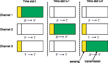

  

  Illustration of multi-channel cognitive radio

  where N^′ is the average number of sensed sub-channels in one time slot.

• Hard constraint: the secondary transmitter can sense only exactly N^′ sub-channels; therefore, the decisions on different sub-channels are mutually correlated. We denote by $\rho ^{t}_{O}$ the probability that the subset of sub-channels $\phantom {\dot {i}\!}O=\left \{i_{1},..., i_{N'}\right \}$ are sensed at time slot t.

On the receiver side, we assume that the secondary receiver can receive over all sub-channels simultaneously, for simplicity. It is interesting to extend the discussion to the situation where the receiver also has only limited capability of sensing (thus, the transmitter and receiver need to play a coordination game). However, this game theoretic situation is beyond the scope of this paper.

2.2 Input and output alphabets

Suppose that all sub-channels share the same discrete input and output alphabets, denoted by $\mathcal {X}$ and $\mathcal {Y}$, respectively. It is easy to extend the analysis to the case where different sub-channels have different input and output alphabets. However, when sub-channel n is idle, the transition probability P _n (y _nm |x _nm ), where $x_{nm}\in \mathcal {X}$ is the m-th input symbol over sub-channel n within a time slot and $y_{nm}\in \mathcal {Y}$ is the m-th output symbol could be different for different sub-channels. We call x _nm and y _nm explicit symbols to distinguish the implicit symbols that will be discussed below.

Besides the explicit input symbols, the input symbol set over sub-channel n also contains Φ (sub-channel n is not sensed) and Ψ (sub-channel n is sensed but found to be busy). We call Φ and Ψimplicit symbols. Therefore, the input alphabet over a sub-channel is given by $\left \{\Phi, \Psi, \mathcal {X}^{M}\right \}$. Similarly, the overall output alphabet is given by $\left \{\Theta, \mathcal {Y}^{M}\right \}$, where Θ means that the receiver receives nothing over the corresponding sub-channel. Then, we denote by X _n (t) and Y _n (t) the overall input and output symbols at sub-channel n during time slot t, respectively. Obviously, the sub-channel maps Φ and Ψ to Θ and maps from $\mathcal {X}$ to $\mathcal {Y}$ (illustrated in Fig. 2a).

Fig. 2

a Input-output mapping. b State transition of sub-channel occupancy

2.3 Input policy

The input policy of the transmitter includes two parts: the probability of sensing a sub-channel and the distribution of explicit input symbols in $\mathcal {X}$ if the sub-channel is found to be idle. We denote by θ _n (t) the input symbol distribution over $\mathcal {X}^{M}$ when the transmitter decides to transmit over sub-channel n. Then, for soft constraint, the joint input probability over sub-channel n at time slot t is given by a _n (t)=(ρ _n (t),θ _n (t)) and the overall input probability is denoted by a(t)=(a₁(t),...,a _N (t)). For hard constraint, the input probability is given by a _O (t)=(ρ _O (t),(θ _n (t)|n∈O)) and the overall input probability is $\mathbf {a}(t)=\left \{a_{O_{i}}\right \}_{i=1,\ldots,\left (\begin {array}{c} N \\ N' \\ \end {array} \right) }$.

2.4 Models of sub-channel occupancy

First, we assume that the occupancies by primary users are independent across different sub-channels. In this paper, the following two possible models are used for the occupancy process on each sub-channel:

• Memoryless model: the occupancy of primary user over a sub-channel is an i.i.d. random process; we denote by $q_{n}^{I}$ the probability that sub-channel n is idle in each time slot.

• Two-state model: the occupancy of primary user over a sub-channel is a two-state (B for busy and I for idle) Markov process, which is illustrated in Fig. 2b; the state of sub-channel n at time slot t is denoted by S _n (t); we denote by $q^{BI}_{n}$ ($q^{IB}_{n}$) the transition probability that the sub-channel n transits from state busy (idle) to state idle (busy); obviously, the memoryless model is a special case of the two-state model when $q^{BI}_{n}+q^{IB}_{n}=1$ and $q^{I}_{n}=q^{BI}_{n}$. We can put the transition probabilities into one matrix, which is given by

  $$\begin{array}{@{}rcl@{}} \mathcal{Q}_{n}=\left(\begin{array}{cc} 1-q_{n}^{IB} & q_{n}^{BI} \\ q_{n}^{IB} & 1-q_{n}^{BI} \\ \end{array} \right). \end{array} $$

  (2)

3 Memoryless sub-channels

When sub-channels are memoryless, it is well known that the sub-channel capacity is given by (note that we ignore all time indices in this section) [6]

$$\begin{array}{@{}rcl@{}} C=\max_{\mathbf{a}}I(X,Y), \end{array} $$

(3)

where a is the set of input distributions which includes the sub-channel selection policy and the distribution of explicit symbols in $\mathcal {X}$ if the corresponding sub-channel is idle. We discuss the optimal input policy with soft constraint and hard constraint separately.

3.1 Soft constraint

Intuitively, the two parts of input policy, namely, sensing probability and sub-channel symbol distribution (in $\mathcal {X}$), can be optimized independently. This can be easily verified by the following decomposition of mutual information (the derivation is in Appendix Appendix A: Decomposition of mutual information):

$$\begin{array}{@{}rcl@{}} I(X,Y)&=&\sum\limits_{n=1}^{N}\rho_{n} q_{n}^{I} \sum\limits_{m=1}^{M}I(x_{mn};y_{mn})+\sum\limits_{n=1}^{N}\rho_{n}q_{n}^{I}\log_{2}\frac{1}{\rho_{n}q_{n}^{I}}\\ &&+\sum\limits_{n=1}^{N}\rho_{n}\left(1-q_{n}^{I}\right)\log_{2}\frac{1}{1-\rho_{n}q_{n}^{I}}\\ &&+\sum\limits_{n=1}^{N}(1-\rho_{n})\log_{2}\frac{1}{1-\rho_{n}q_{n}^{I}}\\ &=&\sum\limits_{n=1}^{N}\rho_{n} q_{n}^{I} \sum\limits_{m=1}^{M}I(x_{mn};y_{mn})+\sum\limits_{n=1}^{N}H\left(\rho_{n}q_{n}^{I}\right), \end{array} $$

(4)

where $H\left (\rho _{n}q_{n}^{I}\right)$ is the entropy of a random variable of coin flipping with head probability $\rho _{n}q_{n}^{I}$.

Obviously, the sub-channel explicit symbol distribution should be optimized in the same way as in traditional memoryless sub-channels, independently of the optimization of sensing probabilities. Therefore, we can focus on the sensing probability by assuming that maximum mutual information of sub-channel symbols, denoted by I_n,max for sub-channel n, has been attained. Throughout this paper, we assume that I_n,max>0, ∀n.

It is easy to show the following proposition which states the optimal sensing probability of each sub-channel (the proof is given in Appendix Appendix B: Proof of Prop. 1).

Proposition 1

Denote by $\left \{\rho _{n}^{*}\right \}$ the capacity-achieving sensing probability. There are two possibilities for $\left \{\rho _{n}^{*}\right \}$:

• When $\sum _{n=1}^{N}\rho _{n}^{*}=N'$, there exists a λ≤0 such that

  $$\begin{array}{@{}rcl@{}} \rho_{n}^{*}=\left\{ \begin{array}{ll} \frac{1}{g_{n}},&\qquad \mathrm{if }\ g_{n}>1\\ 1,&\qquad \mathrm{if }\ g_{n}<1 \end{array} \right., \end{array} $$

  (5)

  where

  $$\begin{array}{@{}rcl@{}} g_{n}=q_{n}^{I}\left(2^{-\frac{\lambda}{q_{n}^{I}}-I_{n,\max}}+1\right). \end{array} $$

  (6)

• When $\sum _{n=1}^{N}\rho _{n}^{*}<N'$, $\rho _{n}^{*}$ is given by

  $$\begin{array}{@{}rcl@{}} \rho_{n}^{*}=\left\{ \begin{array}{ll} \frac{1}{q_{n}^{I}\left(2^{-I_{n,\max}}+1\right)}, \mathrm{if }\ I_{n,\max}\leq -\log_{2}\left(\frac{1}{q_{n}^{I}}-1\right)\\ 1,\mathrm{if }\ I_{n,\max}> -\log_{2}\left(\frac{1}{q_{n}^{I}}-1\right) \end{array} \right.,\\ \end{array} $$

  (7)

Remark 1

An interesting observation is that all sensing probabilities should be positive even if the corresponding $q_{n}^{I}$ and I_n,max are very small. Meanwhile, when $q_{n}^{I}$ and I_n,max are sufficiently large, the sensing probability ρ _n can equal 1. Essentially, this is because $\frac {dH(x)}{dx}\rightarrow \infty$, as x→0; therefore, it is beneficial to keep a positive sensing probability.

Another interesting observation is that it is possible that the constraint $\sum _{n=1}^{N}\rho _{n}\leq N'$ may not be equity, i.e., we would like to give up some sensing opportunity. This seemingly weird conclusion arises from our assumption that the transmitter always transmits something when it finds that the channel is idle. Consider an extreme example: suppose N^′=N and $q_{n}^{*}=1$, i.e., the transmitter has full sensing capability and the channel is always idle. If {I_n,max} are all sufficiently small and we sense all sub-channels (thus transmitting signal over all sub-channels), little information can be conveyed since {I_n,max} are all small. Therefore, it may increase the channel capacity to design a rule to determine whether to transmit over an idle and sensed sub-channel. However, this is beyond the scope of this paper.

3.2 Hard constraint

When hard constraint is applied, exactly N^′ sub-channels are sensed in each time slot. Then, the mutual information of input and output is given by (recall that ρ _O is the probability that sub-channels in subset O are sensed)

$$\begin{array}{@{}rcl@{}} I(X,Y)&=&\sum\limits_{O=\{i_{1},...,i_{N'}\}}\rho_{O}\sum\limits_{K=\{i'_{1},...,i'_{k}\}\subset O}\\ &&\left(\prod\limits_{i\in K}q^{I}_{i}\right)\times\left(\prod\limits_{j\notin K,j\in O}\left(1-q^{I}_{j}\right)\right)\\ &&\times E\left[\log_{2}\frac{P(\mathcal{E}_{XY}(O,K))}{P(\mathcal{E}_{X}(O,K))P(\mathcal{E}_{Y}(K))}\right], \end{array} $$

(8)

where O means the set of sub-channels being sensed and K means the set of sub-channels being sensed and found to be idle. The expectation outside the logarithm is over the randomness of explicit input and output symbols over the idle and sensed sub-channels. The event $\mathcal {E}_{X}(O,K)$ is defined as

$$\begin{array}{@{}rcl@{}} \mathcal{E}_{X}(O,K)&=&\left\{\left\{X_{i}=\Phi|i\notin O\right\},\left\{X_{i}=\Psi|i\notin K,i\in O\right\}\right.\\ &&\left.\left\{\left\{x_{mi}\right\}_{m=1,...,M},X_{i}\in\mathcal{X}^{M}|i\in K\right\}\right\}. \end{array} $$

(9)

Similarly, the event $\mathcal {E}_{Y}(K)$ is defined as

$$ {}\mathcal{E}_{Y}(K)\,=\,\left\{\!\left\{Y_{i}=\Theta|i\notin K\right\}\!,\! \left\{\!\left\{\!y_{mi}\!\right\}_{m=1,...,M}\!,Y_{i}\!\in\!\mathcal{Y}^{M}|i\in K\right\}\!\right\}. $$

(10)

And the joint event $\mathcal {E}_{XY}(O,K)$ is defined as

$$\begin{array}{@{}rcl@{}} \mathcal{E}_{XY}(O,K)=\mathcal{E}_{X}(O,K)\cap \mathcal{E}_{Y}(K). \end{array} $$

(11)

We can further simplify the probability ratio in the logarithm in (8) to

$$\begin{array}{@{}rcl@{}} {}\frac{P(\mathcal{E}_{XY}(O,K))}{P(\mathcal{E}_{X}(O,K))P(\mathcal{E}_{Y}(K))}&=&\frac{P(\mathcal{E}_{Y}(K)|\mathcal{E}_{X}(O,K))}{P(\mathcal{E}_{Y}(K))}\\ &=&\frac{\prod_{n\in K}\prod_{m=1}^{M}P(y_{mn}|x_{mn})}{\prod_{n\in K}\prod_{m=1}^{M}P(y_{mn})}\\ &&\times \frac{1}{P(K)}, \end{array} $$

(12)

where P(K) means the probability that the receiver receives signal on sub-channels belonging to set K.

Then, the expectation in (8) can be decomposed into three parts:

$$ {}E\left[\log_{2}\frac{P(E_{XY}(O,K))}{P(E_{X}(O))P(E_{Y}(K))}\right] =\log_{2}\frac{1}{P(K)}+\sum_{i\in K}I(X_{i},Y_{i}). $$

(13)

There, the mutual information (8) is simplified to

$$\begin{array}{@{}rcl@{}} I(X,Y)=E_{K}\left[\sum\limits_{i\in K}I(X_{i},Y_{i})\right]+H(K), \end{array} $$

(14)

where E _K means the expectation over the randomness of set K and H(K) is the entropy of random set K. Again, we see that the sub-channel symbol distribution should be optimized independently of the sensing probability. Similarly to the soft constraint case, the mutual information is the sum of that of explicit symbols and the entropy of the randomness of the signal existence over sub-channels.

We obtain the following proposition which provides the optimal sensing probability. The proof is provided in Appendix Appendix C: Proof of Prop. 2.

Proposition 2

Denote by $\left \{\rho _{O}^{*}\right \}$ the optimal sensing probability. Then, when

$$\begin{array}{@{}rcl@{}} \sum\limits_{\Omega}2^{\bar{I}_{\Omega}+H_{\Omega}(K)}\geq 1, \end{array} $$

(15)

we have

$$\begin{array}{@{}rcl@{}} \rho_{O}^{*}=\frac{2^{\bar{I}_{O}+H_{O}(K)}}{{\sum\nolimits}_{\Omega}2^{\bar{I}_{\Omega}+H_{\Omega}(K)}}, \end{array} $$

(16)

where

$$\begin{array}{@{}rcl@{}} \bar{I}_{O}=\sum\limits_{K\subset O}P(K|O)\sum\limits_{i\in K}I_{i,\max}, \end{array} $$

(17)

$$\begin{array}{@{}rcl@{}} H_{O}(K)=\sum\limits_{K\subset O}P(K|O)\log_{2}\frac{1}{P(K|O)}, \end{array} $$

(18)

and

$$\begin{array}{@{}rcl@{}} P(K|O)&\triangleq& P\left(\mathrm{sub-channels\ in\ \mathit{K}\ are\ idle}\right.\\ &&\left.| \mathrm{sub-channels\ in\ \mathit{O}\ are\ sensed}\right)\\ &=&\left(\prod_{i\in K}q^{I}_{i}\right)\times\left(\prod_{j\notin K,j\in O}\left(1-q^{I}_{j}\right)\right). \end{array} $$

(19)

When

$$\begin{array}{@{}rcl@{}} \sum\limits_{\Omega}2^{\bar{I}_{\Omega}+H_{\Omega}(K)}< 1, \end{array} $$

(20)

we have

$$\begin{array}{@{}rcl@{}} \rho_{O}^{*}=2^{\bar{I}_{O}+H_{O}(K)}. \end{array} $$

(21)

Remark 2

The difference between the soft constraint and hard constraint cases is in the latter case, no sensing probability can be 1; in contrast, a sensing probability could be 1. The common point is that the sensing probability for every sub-channel should be non-zero. Moreover, the constraint for the sum of sensing probabilities could be an inequality for both cases.

4 Finite-state Markov sub-channels

Due to limited space, we discuss only soft constraint for finite-state Markov sub-channels. The case of hard constraint can be derived in a similar manner. Recall that the state of sub-channel n at time slot t is denoted by S _n (t). Then, the overall state of the system can be given by $\mathbf {S}(t)\triangleq \left (S_{1}(t),...,S_{N}(t)\right)$. We assume that, for each sub-channel n, the transition probabilities $q^{BI}_{n}$ and $q^{IB}_{n}$ are both positive and less than 1. Then, both states of idle and busy are recurrent since they are not affected by the input. Therefore, it is easy to verify that the overall sub-channel is indecomposable and the sub-channel capacity is given by [6]

$$\begin{array}{@{}rcl@{}} C={\lim}_{T\rightarrow\infty}\frac{1}{T}\max_{\mathbf{a}_{1}^{T}}I\left(\mathbf{X}_{1}^{T},\mathbf{Y}_{1}^{T}\right), \end{array} $$

(22)

where (recall that a(t) is the input policy for time slot t)

$$\begin{array}{@{}rcl@{}} \mathbf{a}_{1}^{T}=\left(\mathbf{a}(1),...,\mathbf{a}(T)\right), \end{array} $$

(23)

$$\begin{array}{@{}rcl@{}} \mathbf{X}_{1}^{T}=\left\{X_{n}(t)\right\}_{n=1,...,N;t=1,...,T}, \end{array} $$

(24)

and

$$\begin{array}{@{}rcl@{}} \mathbf{Y}_{1}^{T}=\left\{Y_{n}(t)\right\}_{n=1,...,N;t=1,...,T}. \end{array} $$

(25)

Since the secondary user cannot sense all sub-channels simultaneously, it has only partial information about the overall channel state. Therefore, we can apply the framework of partial observable Markov decision process (POMDP) to study the optimal policy achieving channel capacity. We first define the belief about channel states, converting the partial observable state into a completely observable state. Then, we consider the channel capacity as an average-reward Markov decision problem. The uncountable state space is simplified to a countable one using the special structure of spectrum sensing problem. Finally, the channel capacity is given in stable state probability.

4.1 Belief states

We denote by π _n (t) the a posteriori probability (in our paper, we call it belief about sub-channel n) that sub-channel n is idle in the t-th time slot, conditioned on all previous inputs¹. It is easy to verify that π _n (t) can be computed recursively:

$$\begin{array}{@{}rcl@{}} {}\pi_{n}(t)&=&I(X_{n}(t)=\Psi)q^{BI}_{n}\\ &&+I(X_{n}(t)\in \mathcal{X}^{M})\left(1-q^{IB}_{n}\right)\\ &&+I(X_{n}(t)=\Phi)\pi_{n}(t-1)\left(1-q^{IB}_{n}\right)\\ &&+I(X_{n}(t)=\Phi)\left(1-\pi_{n}(t-1)\right)q^{BI}_{n}, \end{array} $$

(26)

where I is the characteristic function. Obviously, the first term is for the case that sub-channel n is sensed and found to be busy while sub-channel n is sensed but turns out to be idle in the second term. In the last two terms, sub-channel n is not sensed at time slot t and can only be inferred from the a posteriori probability at time slot t−1.

Meanwhile, we denote by μ _n (t) the a posteriori probability that sub-channel n is idle in the t-th time slot, conditioned on all previous outputs. It is easy to verify that μ _n (t) can be computed recursively:

$$\begin{array}{@{}rcl@{}} {}\mu_{n}(t)&=&I\left(Y_{n}(t)\in \mathcal{Y}^{M}\right)\left(1-q^{IB}_{n}\right)\\ &&+I(Y_{n}(t)=\Theta)\mu_{n}(t-1)\left(1-q^{IB}_{n}\right)\\ &&+I(Y_{n}(t)=\Theta)(1-\mu_{n}(t-1))q^{BI}_{n}, \end{array} $$

(27)

where the first term is for the case that the receiver receives explicit symbols over sub-channel n while the following two terms mean that the receiver receives nothing from sub-channel n (the transmitter may have sensed the sub-channel but found that it is busy, or did not sense sub-channel n at all). We assume that the initial probability is given by π _n (0)=μ _n (0).

Using the philosophy in [11], we can consider the beliefs {π _n (t),μ _n (t)}_n=1,...,N as system state at time slot t (note that the system state is different from the state of sub-channels). Then, the POMDP problem is converted to a full information MDP problem since all belief states are known to the transmitter.

4.2 Average award

Using the same argument as in [10], we can obtain

$$\begin{array}{@{}rcl@{}} {}C&=&{\lim}_{n\rightarrow\infty}\max_{\mathbf{a}_{1}^{n}}\frac{1}{T}\sum\limits_{t=1}^{T} \sum\limits_{n=1}^{N}\\ &&\left(H(Y_{n}(t)|\mu_{n}(t))-H(Y_{n}(t)|X_{n}(t),\pi_{n}(t))\right). \end{array} $$

(28)

The following lemma simplifies the difference of the two conditional entropies:

Lemma 1

The following equation holds:

$$\begin{array}{@{}rcl@{}} H(Y_{n}(t)|\mu_{n}(t))&-&H(Y_{n}(t)|X_{n}(t),\pi_{n}(t))\\ &=&P\left(X_{n}(t)\in\mathcal{X}^{M}\right) \sum\limits_{m=1}^{M}I(x_{mn},y_{mn})\\ &&+H(\tilde{Y}_{n}(t)|\mu_{n}(t)), \end{array} $$

(29)

where $\tilde {Y}_{n}(t)$is a binary random variable equaling 1 when $Y_{n}(t)\in \mathcal {Y}^{M}$ and equaling 0 when Y _n (t)=Θ.

Remark 3

Similarly to the memoryless case, the optimization of explicit input distribution is independent of that of sensing probability. Again, we assume that the explicit input distribution has been optimized using traditional approaches and denote by I_n,max the corresponding optimal mutual information over sub-channel n. Then, we focus on only the sensing probabilities.

We assume that the input policy is determined by the belief states, i.e., the sensing probability is determined by {π _n (t)} and {μ _n (t)}. Therefore, the input policy, denoted by a(π(t),μ(t)), is a vector function, and the n-th element, ρ _n (t)=(a(π(t),μ(t))) _n , is the probability of sensing sub-channel n. We assume that the input policy is stationary, i.e., it does not change with time.

Note that the input policy maps from [ 0,1]^2N (the belief states) to the simplex $\sum _{n}^{N}\rho _{n}=N'$ in [ ε,1]^N (the sensing probabilities), where ε is a positive number. The ε preventing the sensing probability from being zero is justified by the following lemma (the proof is straightforward by using the fact that the derivative of function logx is infinite at x=0.)

Lemma 2

For an optimal input policy, the sensing probabilities should be non-zero.

We define the following reward for time slot t:

$$\begin{array}{@{}rcl@{}} &&r(\mathbf{a},S(t))\\ &=&\sum\limits_{n=1}^{N}\left(H(Y_{n}(t)|\mu_{n}(t))-H(Y_{n}(t)|X_{n}(t),\pi_{n}(t))\right), \end{array} $$

(30)

(note that the conditional entropies are completely determined by a(t) and π(t)).

The channel capacity under the constraint of stationary input policy² can be written as

$$\begin{array}{@{}rcl@{}} \hat{C}={\lim}_{T\rightarrow\infty}\max_{\mathbf{\rho}_{1}^{T}}\frac{1}{T}\sum\limits_{t=1}^{T}r(\mathbf{a},S(t)), \end{array} $$

(31)

which is the average award of a controlled Markov process. This motivates us to apply the theory of controlled Markov process to find the optimal input policy.

4.3 Countable state space

The difficulty for analyzing the optimal input policy for the controlled Markov process in (31) is that the state space {π _n (t),μ _n (t)} is uncountable and discretization is needed for optimizing the input policy. However, we can show that the uncountable state space is equivalent to a countable space, thus substantially reducing the complexity.

First, we notice that the belief π _n (t) at time slot t is determined by (suppose that the last time slot (before t) in which the transmitter sensed sub-channel n is t−τ)

$$ {}\pi_{n}(t)=\left\{ \begin{aligned} &\left(\mathcal{Q}_{n}^{\tau}\right)_{11},\qquad \text{if }X_{n}(t-\tau)\in\mathcal{X}^{M}\\ &\left(\mathcal{Q}_{n}^{\tau}\right)_{12},\qquad \text{if }X_{t-\tau}=\Psi\\ &\left(\mathcal{Q}_{n}^{t}\right)_{11}\pi_{n}(0)+\left(\mathcal{Q}_{n}^{t}\right)_{12}(1-\pi_{n}(0))\text{, if }\tau\leq 0 \end{aligned} \right., $$

(32)

with the convention that τ≤0 means sub-channel n has never been sensed (recall that $\mathcal {Q}_{n}$ is the transition matrix of sub-channel n defined in (2)).

Since $\rho _{n}^{IB}+\rho _{n}^{BI}\neq 1$ (otherwise, it degenerates to the memoryless case), $\left (\mathcal {Q}_{n}^{t_{1}}\right)_{11}\neq \left (\mathcal {Q}_{n}^{t_{2}}\right)_{12}$, for t₁,t₂>0 almost surely. Also, $\left (\mathcal {Q}_{n}^{t}\right)_{11}\pi _{n}(0)+\left (\mathcal {Q}_{n}^{t}\right)_{12}(1-\pi _{n}(0))$ is equal to $\left (\mathcal {Q}_{n}^{t_{1}}\right)_{11}$ or $\left (\mathcal {Q}_{n}^{t_{1}}\right)_{12}$ for only countable cases, which is of measure zero. Therefore, we can determine the last time slot in which sub-channel n is sensed before time slot t from π _n (t) almost surely.

Similarly, the belief μ _n (t) at time slot t is determined by (suppose that the last time slot, denoted by t−δ, in which sub-channel n is sensed and found to be idle (i.e., $Y_{n}(t)\in \mathcal {Y}^{M}$))

$$ {}\mu_{n}(t)=\left\{ \begin{array}{ll} \left(\mathcal{Q}_{n}^{\delta}\right)_{11},\qquad \text{if }X_{n}(t-\delta)\in\mathcal{X}^{M}\\ \left(\mathcal{Q}_{n}^{t}\right)_{11}\pi_{n}(0)+\left(\mathcal{Q}_{n}^{t}\right)_{12}(1-\pi_{n}(0))\text{, if }\delta\leq 0 \end{array} \right., $$

(33)

with the convention that δ≤0 means the receiver has never received signal over sub-channel n before time t. Similarly, μ _n (t) is equivalent to δ almost surely.

When the initial state for sub-channel n is π _n (0)=1 and μ _n (0)=1, π _n (t) is either $\left (\mathcal {Q}_{n}^{t_{1}}\right)_{11}$ or $\left (\mathcal {Q}_{n}^{t_{2}}\right)_{12}$, where t₁ and t₂ are integers, due to (32), and μ _n (t) can only be $\left (\mathcal {Q}_{n}^{t_{3}}\right)_{11}$, where t₃ is an integer, due to (33). This means that the possible values of π _n (t) and μ _n (t) are countable. Then, each sub-state (π _n (t),μ _n (t)) is equivalent to a 3-tuple (S _n (τ),τ,δ) where t−τ is the last time slot in which sub-channel n is sensed and t−δ is the last time slot in which sub-channel n is sensed and found to be idle (obviously, δ≤τ). Therefore, the state space [ 0,1]^N degenerates to a discrete state space

$$\begin{array}{@{}rcl@{}} \mathbf{\Xi}=\left\{\left\{B,I\right\}\times \left\{(\tau,\delta)|\tau\in\mathbb{N},\delta\in\mathbb{N},\tau\leq \delta\right\}\right\}^{N}. \end{array} $$

(34)

And we denote by ξ(t) and ξ _n (t), the state and the sub-state for sub-channel n at time slot t.

However, it loses generality to assume π _n (0)=1 or 0, ∀n. Fortunately, we can show that the longer-term average reward is a constant dependent on only the control strategy, regardless the initial state. Toward this, we can apply Theorem 1 in Appendix Appendix E: Markov control uncountable state space [11]. The following lemma verifies the assumptions in Theorem 1, whose proof is given in Appendix Appendix F: Proof of Lemma 3.

Lemma 3

Assumptions 1 and 2 hold for the controlled Markov process of spectrum sensing.

Applying the conclusion in Theorem 1 and Lemma 3, we obtain the following proposition, which converts the finite state sub-channel into a memoryless one:

Proposition 3

The sub-channel capacity is independent of the initial state and is given by

$$\begin{array}{@{}rcl@{}} {}C=\max_{\Delta}\sum\limits_{\xi\in \mathbf{\Xi}} \sum\limits_{n=1}^{N}\left(H(Y_{n}|\xi)-H(Y_{n}|X_{n},\xi)\right)\Delta(\xi), \end{array} $$

(35)

where Δis the stable probability of belief state ξ.

The stable probability Δ is determined by the following equation:

$$\begin{array}{@{}rcl@{}} \Delta(\xi)=\sum\limits_{\xi'\rightarrow\xi}\Delta(\xi')\prod\limits_{n=1}^{N}P(\xi_{n}|\xi'), \end{array} $$

(36)

where ξ^′ and ξ are both overall state, ξ _n is the state of sub-channel n, ξ^′→ξ means that ξ^′ is a legal state in the previous time slot when the current state is ξ and P(ξ _n |ξ^′) is the transition probability, which is given by

$$\begin{array}{@{}rcl@{}} P(\xi_{n}|\xi')=1-\left(\mathbf{a}(\xi')\right)_{n}, \end{array} $$

(37)

if ξ _n =(x,τ,δ) and ξn′=(x,τ−1,δ−1) (i.e., sub-channel n is not sensed), and

$$\begin{array}{@{}rcl@{}} P(\xi_{n}|\xi')=\left(\mathbf{a}(\xi')\right)_{n}, \end{array} $$

(38)

otherwise. Then, the sensing probability can be optimized numerically, which is out of the scope of this paper.

4.4 Myopic strategy

The above approaches based on POMDP can achieve theoretically optimal performance. However, they can hardly be implemented when the number of channels becomes large, even if we keep only finitely many states in (33). For example, if we keep only two states for each channel, there will be 2^N overall states. When N=20, which is used in the numerical simulation section of this paper, the computational and memory costs will be prohibitive.

Hence, we propose a practical approach based on the myopic strategy, namely, to maximize the expected throughput in the next time slot. We consider the belief π _n (t) as the true idle probability of channel n. Then, we apply the scheduling strategy in Prop. 1 (for the soft constraint case) or in Prop. 2 (for the hard constraint case).

5 Numerical results

In this section, we provide numerical simulation results to demonstrate the mathematical analysis conclusions.

5.1 Simulation setup

We assume that there are totally 20 channels (Table 1). We further assume that each channel is a symmetric binary channel with identical channel capacity. We will test the performance for different values of individual channel capacity. Note that I_n,max is the maximum mutual information of sub-channel symbols for sub-channel n. We assume that I_n,max is identical for all channels, whose quantity is called the capacity index, whose unit is bits/second.

Table 1 Simulation setup

5.2 Memoryless channels

We first consider the memoryless channels.

5.2.1 Soft constraint

We assume that the secondary user can averagely sense two channels at a time, namely, N^′=2. We consider three setups of idle probabilities: (1) uniformly ranging from 0.1 to 0.9, (2) uniformly ranging from 0.1 to 0.3, and (3) uniformly ranging from 0.8 to 0.9. We tested the capacity for 20 values of I_n,max, the first ten range from 0.1 to 1 while the last ten range from 5 to 50. The final capacity is illustrated in Fig. 3.

Fig. 3

Capacity versus the index of I_n,max

A simple approach is to always sense the most idle channel. We use the performance of this simple scheme as the baseline. The relative performance gain, defined as

$$\begin{array}{@{}rcl@{}} \text{relative gain}=\frac{I_{opt}(X;Y)-\text{baseline}}{\text{baseline}}. \end{array} $$

(39)

The relative gain corresponding to the setups in Fig. 3 is shown in Fig. 4. We observe that, when the individual capacity I_n,max is low, the performance gain is very high; however, when I_n,max is large, the performance gain is negligible. Hence, this implies that the proposed scheme be suitable for low signal-to-noise-ratio (SNR) case. For high-quality channels, the traditional spectrum access scheme is sufficiently good.

Fig. 4

Relative performance gain versus the index of I_n,max

5.2.2 Hard constraint

Figure 5 shows the performance loss of the hard constraint (relative to the soft constrained case) in the same setups as those in Fig. 3. We observe that the performance loss is significant due to the hard constraint. When I_n,max is large, the performance loss becomes much smaller.

Fig. 5

Relative performance loss of hard constraint versus the index of I_n,max

5.3 Markov channels

We tested the Markov channel case. We use the same setup of I_n,max as that in Fig. 3. We further assume that all the channels have the same state transition probability. We have the following three setups for the transition probabilities: $\left (q_{n}^{IB},q_{n}^{BI}\right)=(0.1,0.9)$ or (0.5,0.5) or (0.5,0.9).

Then, we applied the myopic strategy and obtained the average capacity in 10,000 time slots. We also tested the performance of the traditional coding scheme, together with the strategy of selecting the most probable channels, and use it as the baseline. Then, the relative performance gain of the myopic approach over the baseline is given in Fig. 6. We can also observe a positive performance gain when the channel selection is also used to convey information. Again, the gain drops when I_n,max becomes large.

Fig. 6

Relative performance loss of hard constraint versus the index of I_n,max in Markov channel

6 Conclusions and open problems

In this paper, we have analyzed the channel capacity in multi-channel cognitive radio systems. Both memoryless and finite state sub-channels have been studied. The separation principle for the optimizations of input distribution over individual sub-channels and sub-channel selection has been proved. For the case of finite state sub-channels, the capacity optimization problem is considered as an average reward maximizing one and it has been shown that under the constraint of stationary input policy, the channel capacity is determined by the static distribution of state occupancy probabilities. The performance gain due to the proposed scheme has been demonstrated using numerical simulations.

Our work in this paper can be extended in the following lines:

• Extension from single-user to multi-user situation, in which the capacity region needs to be studied.

• Considering the sensor error, or modeling the sub-channels as hidden Markov models (HMMs).

• Considering the case of limited receiving capability, i.e., the receiver can receive over a subset of sub-channels, for which game theory needs to be applied since the decision concerns two players.

7 Appendix A: Decomposition of mutual information

For the soft constraint with memoryless sub-channels, we have

$$ {}\begin{array}{ccl} I(X,Y) &=&\sum\limits_{n=1}^{N}\sum\limits_{m=1}^{M}\sum\limits_{x_{mn}\in\mathcal{X},y_{mn}\in\mathcal{Y}}P\!\left(x_{mn},y_{mn},X_{n}\in\mathcal{X}^{M}\!,Y_{n}\in\mathcal{Y}^{M}\right)\\ &&\times\log_{2}\frac{P\left(x_{mn},y_{mn},X_{n}\in\mathcal{X}^{M},Y_{n}\in\mathcal{Y}^{M}\right)}{P\left(x_{mn},X_{n}\in\mathcal{X}^{M}\right)P\left(y_{mn},Y_{n}\in\mathcal{Y}^{M}\right)}\\ &&+\sum\limits_{n=1}^{N}P(X_{n}=\Psi,Y_{n}=\Theta)\log_{2}\left(\frac{P(X_{n}=\Psi,Y_{n}=\Theta)}{P(X_{n}=\Psi)P(Y_{n}=\Theta)}\right)\\ &&+\sum\limits_{n=1}^{N}P(X_{n}=\Phi,Y_{n}=\Theta)\log_{2}\left(\frac{P(X_{n}=\Phi,Y_{n}=\Theta)}{P(X_{n}=\Phi)P(Y_{n}=\Theta)}\right). \end{array} $$

(40)

The first term in (40) can be simplified as below:

$$ {}\begin{aligned} \sum\limits_{m=1}^{M}&\sum\limits_{x_{mn}\in\mathcal{X},y_{mn}\in\mathcal{Y}}P\left(x_{mn},y_{mn},X_{n}\in\mathcal{X}^{M},Y_{n}\in\mathcal{Y}^{M}\right)\\ &\quad\times\log_{2}\frac{P\left(x_{mn},y_{mn},X_{n}\in\mathcal{X}^{M},Y_{n}\in\mathcal{Y}^{M}\right)}{P\left(x_{mn},X_{n}\in\mathcal{X}^{M}\right)P\left(y_{mn},Y_{n}\in\mathcal{Y}^{M}\right)}\\ &=P\left(X_{n}\in\mathcal{X}^{M},Y_{n}\in\mathcal{Y}^{M}\right)\\ &\quad\times\sum\limits_{m=1}^{M}\sum\limits_{x_{mn}\in\mathcal{X},y_{mn}\in\mathcal{Y}}P\left(x_{mn},y_{mn}|X_{n}\in\mathcal{X}^{M},Y_{n}\in\mathcal{Y}^{M}\right)\\ &\quad\times\log_{2}\left(\frac{P\left(x_{mn},y_{mn}|X_{n}\in\mathcal{X}^{M},Y_{n}\in\mathcal{Y}^{M}\right)}{P\left(x_{mn}|X_{n}\in\mathcal{X}^{M}\right) P\left(y_{mn}|Y_{n}\in\mathcal{Y}^{M}\right)}\right.\\ &\quad\times\left.\frac{P\left(X_{n}\in\mathcal{X}^{M},Y_{n}\in\mathcal{Y}^{M}\right)}{P\left(X_{n}\in\mathcal{X}^{M}\right) P\left(Y_{n}\in\mathcal{Y}^{M}\right)} \right)\\ &=P\left(X_{n}\in\mathcal{X}^{M},Y_{n}\in\mathcal{Y}^{M}\right)\sum\limits_{m=1}^{M}I\left(x_{mn},y_{mn}\right)\\ &\quad+\!P\left(X_{n}\in\mathcal{X}^{M},Y_{n}\in\mathcal{Y}^{M}\right)\log_{2} \frac{P\left(X_{n}\in\mathcal{X}^{M},Y_{n}\in\mathcal{Y}^{M}\right)}{P\left(X_{n}\in\mathcal{X}^{M}\right)\!P\!\left(Y_{n}\in\mathcal{Y}^{M}\right)}\\ &=\rho_{n} q_{n}^{I}\sum\limits_{m=1}^{M}I(x_{mn};y_{mn})+\rho_{n}q_{n}^{I}\log_{2}\frac{1}{\rho_{n}q_{n}^{I}}, \end{aligned} $$

(41)

where we applied the following facts:

$$\begin{array}{@{}rcl@{}} P\left(X_{n}\in\mathcal{X}^{M},Y_{n}\in\mathcal{Y}^{M}\right)=\rho_{n} q_{n}^{I}, \end{array} $$

(42)

and (notice that $P\left (Y_{n}\in \mathcal {Y}^{M}|X_{n}\in \mathcal {X}^{M}\right)=1$ and $P\left (Y_{n}\in \!\right. \left.\mathcal {Y}^{M}\right)=\rho _{n}q_{n}^{I}$.)

$$\begin{array}{@{}rcl@{}} \frac{P\left(X_{n}\in\mathcal{X}^{M},Y_{n}\in\mathcal{Y}^{M}\right)}{P\left(X_{n}\in\mathcal{X}^{M}\right)P\left(Y_{n}\in\mathcal{Y}^{M}\right)} &=&\frac{P\left(Y_{n}\in\mathcal{Y}^{M}|X_{n}\in\mathcal{X}^{M}\right)}{P\left(Y_{n}\in\mathcal{Y}^{M}\right)}\\ &=&\frac{1}{\rho_{n}q_{n}^{I}}. \end{array} $$

(43)

The second term is given by

$$\begin{array}{@{}rcl@{}} P(X_{n}=\Psi,Y_{n}=\Theta)&\log_{2}&\left(\frac{P(X_{n}=\Psi,Y_{n}=\Theta)}{P(X_{n}=\Psi)P(Y_{n}=\Theta)}\right)\\ &=&P(Y_{n}=\Theta|X_{n}=\Psi)P(X_{n}=\Psi)\\ &&\times\log_{2}\left(\frac{P(Y_{n}=\Theta|X_{n}=\Psi)}{P(Y_{n}=\Theta)}\right)\\ &=&\rho_{n}\left(1-q_{n}^{I}\right)\log_{2}\frac{1}{1-\rho_{n}q_{n}^{I}}, \end{array} $$

(44)

where we used the following facts: P(Y _n =Θ|X _n =Ψ)=1, $P(Y_{n}=\Theta)=1-\rho _{n}q_{n}^{I}$ and $P(X_{n}=\Psi)=\rho _{n}\left (1-q_{n}^{I}\right)$.

The third term is given by

$$\begin{array}{@{}rcl@{}} P(X_{n}=\Phi,Y_{n}=\Theta)&\log_{2}&\left(\frac{P(X_{n}=\Phi,Y_{n}=\Theta)}{P(X_{n}=\Phi)P(Y_{n}=\Theta)}\right)\\ &=&P(Y_{n}=\Theta|X_{n}=\Phi)P(X_{n}=\Phi)\\ &&\times\log_{2}\left(\frac{P(Y_{n}=\Theta|X_{n}=\Phi)}{P(Y_{n}=\Theta)}\right)\\ &=&\left(1-\rho_{n}\right)\log_{2}\frac{1}{1-\rho_{n}q_{n}^{I}}, \end{array} $$

(45)

where we have used the facts P(Y _n =Θ|X _n =Φ)=1 and P(X _n =Φ)=1−ρ _n . This concludes the decomposition in (4).

8 Appendix B: Proof of Prop. 1

Proof

The proof is straightforward by taking derivative of I(X,Y) with respect to ρ _n as well as considering the constraint, which is given by

$$\begin{array}{@{}rcl@{}} \frac{\partial I(X,Y)}{\partial \rho_{n}}+\lambda+\omega_{n}-\mu_{n}&=&q_{n}^{I}I_{n,\max}-q_{n}^{I}\log_{2}\left(q_{n}^{I}\rho_{n}\right)\\ &&-\frac{q_{n}^{I}}{\log_{e}2} +q_{n}^{I}\log_{2}\left(1-q_{n}^{I}\rho_{n}\right)\\ &&+\frac{q_{n}^{I}}{\log_{e}2}+\lambda+\omega_{n}-\mu_{n}, \end{array} $$

(46)

where λ<0 is the Lagrange multiplier for the constraint $\sum _{n}^{N}\rho _{n}=N$, ω _n ≤0 is the Lagrange factor for the constraint ρ _n ≤1 and μ _n ≤0 is the Lagrange factor for the constraint ρ _n ≥0.

ρ _n cannot be zero since log2ρ _n becomes negatively infinite and the equation $\frac {\partial I(X,Y)}{\partial \rho _{n}}=0$ cannot be satisfied. Therefore, μ _n must be zero. The conclusion follows from Karush-Kuhn-Tucker condition. □

9 Appendix C: Proof of Prop. 2

Proof

We can take the derivative of I(X,Y) with respect to ρ _O as well as the constraint, which is given by

$$\begin{array}{@{}rcl@{}} \frac{\partial I(X,Y)}{\partial \rho_{O}}+&\lambda&+\omega_{O}-\mu_{O}\\ &=&\sum\limits_{K\subset O}P(K|O)\sum\limits_{k\in K}I_{k,\max}\\ &&+\sum\limits_{K\subset O}P(K|O)\log_{2}\frac{1}{P(K|O)\rho_{O}}\\ &&-\sum\limits_{K\subset O}P(K|O)\log_{2}e+\lambda+\omega_{O}-\mu_{O}\\ &=&\bar{I}_{O}+H_{O}(K)-\log_{2}e-\log_{2}\rho_{O}\\ &&+\lambda+\omega_{O}-\mu_{O}, \end{array} $$

(47)

where λ≤0 is the Lagrange factor for the constraint $\sum _{O}\rho _{O}^{*}\leq 1$, ω _O ≤0 is the Lagrange factor for the constraint ρ _O ≤1, and μ _O ≤0 is the Lagrange factor for the constraint ρ _O ≥1. Note that P(K|O) is defined as

$$\begin{array}{@{}rcl@{}} P(K|O)&=&P(\text{sub-channels in \textit{K} are idle while}\\ && \text{all other sub-channels in \textit{O} are busy}). \end{array} $$

(48)

And we define

$$\begin{array}{@{}rcl@{}} \bar{I}_{O}=\sum\limits_{K\subset O}P(K|O)\sum\limits_{i\in K}I_{i,\max}, \end{array} $$

(49)

$$\begin{array}{@{}rcl@{}} H_{O}(K)=\sum\limits_{K\subset O}P(K|O)\log_{2}\frac{1}{P(K|O)}. \end{array} $$

(50)

Obviously, ρ _O cannot be zero since log2ρ _O becomes negatively infinite and the equation $\frac {\partial I(X,Y)}{\partial \rho _{O}}=0$ cannot be satisfied. Consequently, ρ _O cannot be 1 since this makes other sensing probabilities zero, which contradicts the previous conclusion of non-zero sensing probability. Therefore, both ω _O and μ _O must be zero and the equation $\frac {\partial I(X,Y)}{\partial \rho _{O}}=0$ becomes

$$\begin{array}{@{}rcl@{}} \bar{I}_{O}+H_{O}(K)-\log_{2}e-\log_{2}\rho_{O} +\lambda=0. \end{array} $$

(51)

Then, when $\sum _{O}\rho _{O}=1$ is satisfied, we have

$$\begin{array}{@{}rcl@{}} \rho_{O}=2^{\lambda+\bar{I}_{O}+H_{O}(K)-\log_{2}e}. \end{array} $$

(52)

It is easy to obtain

$$\begin{array}{@{}rcl@{}} 2^{-\lambda}=\sum\limits_{O}2^{\bar{I}_{O}+H_{O}(K)-\log_{2}e}. \end{array} $$

(53)

Recall that the constraint λ ≤0 requires $\sum _{\Omega }2^{\bar {I}_{\Omega }+H_{\Omega }(K)}\geq 1$. Otherwise, $\sum _{O}\rho _{O}=1$ is not satisfied and λ=0. This concludes the proof. □

10 Appendix D: Proof of Lemma 1

Proof

For the entropy conditioned on μ _n (t), we have

$$\begin{array}{*{20}l} {}H(Y_{n}(t)|\mu_{n}(t)) &=E[-\log_{2}\left(P(Y_{n}(t)|\mu_{n}(t))\right)]\\ &=\int_{0}^{1}\sum\limits_{Y_{n}(t)\in \mathcal{Y}^{M}}P(Y_{n}(t),\mu_{n}(t))\\ &\quad\times \left(-\log_{2}\left(P(Y_{n}(t)|\mu_{n}(t))\right)\right)dP(\mu_{n}(t))\\ &\quad+\int_{0}^{1}P(Y_{n}(t)=\Theta,\mu_{n}(t))\\ &\quad\times\left(\!- \!\log_{2}\left(\!P(Y_{n}(t) \!= \!\Theta|\mu_{n}(t) \!) \!\right) \!\right) \!dP(\mu_{n}(t)),\\ \end{array} $$

(54)

where we used the facts p(Y _n (t)|S _n (t)=B)=0 when $Y_{n}(t)\in \mathcal {Y}^{M}$ and p(Y _n (t)=Θ|S _n (t)=B)=1.

The first term in (54) can be decomposed to

$$\begin{array}{*{20}l} {}\int_{0}^{1}\sum\limits_{Y_{n}(t)\in \mathcal{Y}^{M}}&P(Y_{n}(t),\mu_{n}(t))\\ &\times\left(-\log_{2}\left(P(Y_{n}(t)|\mu_{n}(t))\right)\right)dP(\mu_{n}(t))\\ =&\int_{0}^{1}P(Y_{n}(t)\in \mathcal{Y}^{M},\mu_{n}(t))\\ &\times\sum\limits_{y_{mn}}\prod\limits_{m=1}^{M}p\left(y_{mn}|Y_{n}(t)\in \mathcal{Y}^{M}\right)\\ &\left(\,-\,\sum_{m=1}^{M}\!\log_{2}\!\left(P(y_{mn}|Y_{n}(t)\!\in\! \mathcal{Y}^{M})\right)\!\right)\!dP(\mu_{n}(t))\\ &+\int_{0}^{1}P(Y_{n}(t)\in \mathcal{Y}^{M},\mu_{n}(t))\\ &\times\left(-\log_{2}\left(P(Y_{n}\!(t)\in\mathcal{Y}^{M}|\mu_{n}(t))\right)\right)dP(\mu_{n}(t))\\ =&P\left(Y_{n}(t)\in \mathcal{Y}^{M}\right)\\ &\times\sum\limits_{y_{mn}}\prod\limits_{m=1}^{M}p\left(y_{mn}|Y_{n}(t)\in \mathcal{Y}^{M}\right)\\ &\left(-\sum\limits_{m=1}^{M}\log_{2}\left(P\left(y_{mn}|Y_{n}(t)\in \mathcal{Y}^{M}\right)\right)\right)\\ &+\int_{0}^{1}P(Y_{n}(t)\in \mathcal{Y}^{M},\mu_{n}(t))\\ &\times\left(-\log_{2}\left(P(Y_{n}(t)\in\mathcal{Y}^{M}|\mu_{n}(t))\right)\right)dP(\mu_{n}(t)).\\ \end{array} $$

(55)

We also have

$$\begin{array}{@{}rcl@{}} H(\!\!&Y_{n}&\!\!(t)|X_{n}(t),\pi_{n}(t))\\ =&&{}E\left[-\log_{2}\left(p(Y_{n}(t)|X_{n}(t),\pi_{n}(t))\right)\right]\\ =&&{}\int_{0}^{1}\sum\limits_{Y_{n}(t)\in\mathcal{Y}^{M},X_{n}(t)\in\mathcal{X}^{M}}P(Y_{n}(t),X_{n}(t),\pi_{n}(t))\\ &\times&\!\!\!\left(-\log_{2}\left(P(Y_{n}(t)|X_{n}(t),\pi_{n}(t)\right)\right)d(p(\pi_{n}(t)))\\ &+&\!\!\!\int_{0}^{1}P(Y_{n}(t)=\Theta,X_{n}(t)=\Psi,\pi_{n}(t))\\ &\times&\!\!\!\left(-\!\log_{2}\!\left(P(Y_{n}(t)\,=\,\Theta|X_{n}(t)\,=\,\Psi\!,\pi_{n}(t))\!\right)\!\right)\!d\!(p(\pi_{n}(t)\!)\!)\\ &+&\!\!\!\int_{0}^{1}P(Y_{n}(t)=\Theta,X_{n}(t)=\Phi,\pi_{n}(t))\\ &\times&\!\!\!\left(-\!\log_{2}\!\left(P(Y_{n}(t)=\Theta|X_{n}(t)=\Phi,\pi_{n}(t))\right)\right)d(p(\pi_{n}(t)))\\ =&&{}P(X_{n}(t)\in\mathcal{X}^{M})\sum\limits_{m=1}^{M}\sum\limits_{x_{nm},y_{nm}}\log_{2}\left(p(y_{nm}|x_{nm})\right). \end{array} $$

(56)

Note that, in the second equation, the last two terms are both zero since p(Y _n (t)=Θ|X _n (t)=Ψ,π _n (t))=1 and P(Y _n (t)=Θ|X _n (t)=Φ,π _n (t))=1.

Then, we have

$$\begin{array}{@{}rcl@{}} && H(Y_{n}(t)|\mu_{n}(t))-H(Y_{n}(t)|X_{n}(t),\pi_{n}(t))\\ &=&P \left(X_{n}(t)\in\mathcal{X}^{M}\right) \sum\limits_{m=1}^{M}I(x_{mn},y_{mn})\\ &&+\int_{0}^{1}P(Y_{n}(t)=\Theta,\mu_{n}(t))\\ &&\times\left(-\log_{2}\left(P(Y_{n}(t)=\Theta|\mu_{n}(t))\right)\right)dP(\mu_{n}(t))\\ &&+\int_{0}^{1}P\left(Y_{n}(t)\in\mathcal{Y}^{M},\mu_{n}(t)\right)\\ &&\times\left(-\log_{2}\left(P(Y_{n}(t)\in\mathcal{Y}^{M}|\mu_{n}(t))\right)\right)dP(\mu_{n}(t)).\\ \end{array} $$

(57)

This concludes the proof. □

11 Appendix E: Markov control uncountable state space

Consider a discrete-time Markov control model characterized by a four-tuple (S,A,T,r):

• State space S is a Borel space (defined as a Borel subset of a complete separable metric space);

• Action space A is also a Borel space; each state s in the state space S is associated with a non-empty measurable subset A(s), whose elements are legal actions for state s; we assume that state-action pair set $\mathbf {K}\triangleq \left \{(s,a)|s\in \mathbf {S}, a\in \mathbf {A}\right \}$ is measurable;

• T is the transition law, whose elements are denoted by T(B|k), where $B\in \mathcal {B}(\mathbf {A})$ and k∈K;

• r is the reward function mapping from K to $\mathbb {R}$.

Our task is to maximize the average reward, which is given by

$$\begin{array}{@{}rcl@{}} J(\delta,s)\triangleq \lim\inf_{T\rightarrow\infty}E\left[\sum\limits_{t=1}^{T}r(s_{t},a_{t})\right], \end{array} $$

(58)

where δ is a policy and s is the initial state.

We need the following assumptions (Assumptions 2.1 in [11]):

Assumption 1

(Regularity)

• For each state s∈S, A(s) is a non-empty compact subset of A;

• The reward function r(x,a) is bounded and continuous for a∈A(s);

• $\int g(y)\mathbf {T}(dy|s,a)$ is a continuous function in a∈A(s) for each s∈S and for each function g∈B(S).

We also need the following ergodicity assumption (Assumption 3.1 (1) in [11]):

Assumption 2

(Ergodicity)There exists a state s^∗∈S and a positive number c such that

$$\begin{array}{@{}rcl@{}} \mathbf{T}(s^{*}|k)>c,\qquad \forall k\in \mathbf{K}. \end{array} $$

(59)

Combining Theorem 2.2, Lemma 3.3 and Corollary 3.6 in [11], we have the following theorem:

Theorem 1

The following statement hold:

• If the Ergodicity Assumption holds, then, for any arbitrary policy a, there exists an invariant measure p _a , i.e. the unique invariant probability measure satisfying

  $$\begin{array}{@{}rcl@{}} p_{\mathbf{a}}(B)=\int_{\mathbf{S}}\mathbf{T}_{f}(B|s)p_{f}(dx), \end{array} $$

  (60)

  for all $B\in \mathcal {B}(S)$, and the average reward function J(f,a) is a constant J(f) (thus being independent of initial state s), which is given by

  $$\begin{array}{@{}rcl@{}} J(f)=\int r(y,\mathbf{a}(y))p_{\mathbf{a}}(dy), \end{array} $$

  (61)

• If both the Regularity Assumption and Ergodicity Assumption hold, then there exists a constant J^∗ and a function h^∗ in B(S) satisfying the following Optimality Equation, ∀s∈S,

  $$\begin{array}{@{}rcl@{}} {}J^{*}+h^{*}(s)=\max_{a\in A(s)}\left\{r(s,a)+\int_{\mathbf{S}}h^{*}(y)\mathbf{T}(dy|s,a)\right\}. \end{array} $$

  (62)

• Consider a Markov policy {a _t } such that it maximizes the right hand side of the following equation:

  $$\begin{array}{@{}rcl@{}} h^{*}_{t}(s)=\max_{a\in\mathbf{A}(s)}\left\{r(s,a)+\int h_{t-1}(y)\mathbf{T}(dy|s,a)\right\}, \end{array} $$

  (63)

  where h₀∈B(S) is arbitrary, i.e.

  $$\begin{array}{@{}rcl@{}} h_{t}(s)=r(s,\mathbf{a}_{t}(s))+\int h_{t-1}(y)\mathbf{T}(dy|s,f_{t}(s)), \end{array} $$

  (64)

  then, the policy using a _t at time slot t is optimal.

12 Appendix F: Proof of Lemma 3

Proof

We first verify the items in Assumption 1 (regularity):

• For each state π, the corresponding set of action a(π) is a point in [ ε,1]^N, which is compact;

• From (30), the reward function r(s,a) is bounded by

  $$\begin{array}{@{}rcl@{}} &&\left|r(\mathbf{a}(t),\pi(t))\right|\\ &\leq&\sum\limits_{n=1}^{N}H(Y_{n}(t)|\mu_{n}(t))\\ &\leq&\sum\limits_{n=1}^{N}I_{n,\max}+n. \end{array} $$

  (65)

  The continuity can be obtained directly from (54) and (56);

• Note that the action space A(s) for state s∈S is the hyper-rectangle [ ε,1]^N. Consider two policies a and a^′ corresponding to state s=π and ∥a−a^′∥=δf. If $\pi _{n}=\left (\mathcal {Q}_{n}^{r}\right)_{11}$ (sub-channel n is sensed r time slots ago and is found idle), we have

  $$\begin{array}{@{}rcl@{}} P\left(\pi_{n}(t+1)=\left(\mathcal{Q}_{n}^{r+1}\right)_{11}\right)=1-\mathbf{a}_{n}(\pi), \end{array} $$

  (66)

  and

  $$\begin{array}{@{}rcl@{}} P\left(\pi_{n}(t+1)=\left(\mathcal{Q}_{n}^{1}\right)_{11}\right)=\mathbf{a}_{n}(\pi)\pi_{n}(t), \end{array} $$

  (67)

  and

  $$\begin{array}{@{}rcl@{}} P\left(\pi_{n}(t+1)=\left(\mathcal{Q}_{n}^{1}\right)_{12}\right)=\mathbf{a}_{n}(\pi)(1-\pi_{n}(t)). \end{array} $$

  (68)

  The change of the probability is of order O(δf). It is easy to verify the same conclusion for the cases $\pi _{n}(t)=\left (\mathcal {Q}_{n}^{r}\right)_{12}$ and $\pi _{n}(t)=\left (\mathcal {Q}_{n}^{t}\right)_{11}\pi _{n}(0) +\left (\mathcal {Q}_{n}^{t}\right)_{12}(1-\pi _{n}(0))$. Therefore,

  $$\begin{array}{@{}rcl@{}} |\mathbf{T}(dy|\mathbf{a},s)-\mathbf{T}(dy|\mathbf{a}',s)|=O(\delta f). \end{array} $$

  (69)

  Then, we obtain the continuity of $\int g(y)\mathbf {T}(dy|s,a)$ using the assumption that g is a bounded function.

Next, we verify Assumption 2 (ergodicity). We set

$$\begin{array}{@{}rcl@{}} s^{*}=\left\{\pi_{n}(t)=\left(\mathcal{Q}_{n}^{1}\right)_{11}\right\}_{n=1,...,N}, \end{array} $$

(70)

i.e., all sub-channels are sensed. Since a _n ≥ε, the probability of sensing sub-channel n is always positive, which implies

$$\begin{array}{@{}rcl@{}} \mathbf{T}(s^{*}|k)\geq \epsilon^{n},\qquad \forall k\in \mathbf{K}. \end{array} $$

(71)

This concludes the proof. □

References

V Anantharam, S Verdú, Bits through queues. IEEE Trans. Inform. Theory. 42:, 4–19 (1996).
S Bhattarai, J Park, B Gao, K Bian, W Lehr, An overview of dynamic spectrum sharing: ongoing initiatives, challenges, and a roadmap for future research. IEEE Trans. Cogn. Commun. Netw. 2(2), 110–125 (2016).
R Combes, A Proutiere, Dynamic rate and channel selection in cognitive radio systems. IEEE J. Sel. Areas Commun. 33.5:, 910–921 (2015).
M Elalem, L Zhao, in IEEE International Conference on Wireless Communications and Networking Conference (WCNC2013). Effective capacity and interference constraints in multichannel cognitive radio network (IEEEShanghai, 2013).
S Eryigit, T Tugcu, in Cognitive Radio Oriented Wireless Networks and Communications (CROWNCOM), 2012 7th International ICST Conference on. Joint channel and user selection for transmission and sensing in cognitive radio networks (IEEEkunming, 2012).
RG Gallager, Information Theory and Reliable Communication (Wiley, New York, 1968).
Y Gao, et al, in Signal Processing (ICSP), 2016 IEEE 13th International Conference on. Effective capacity of cognitive radio systems (IEEEChengdu, 2016).
L Gao, L Duan, J Huang, Two-sided matching based cooperative spectrum sharing. IEEE Trans. Mob. Comput. 16(2), 538–551 (2017).
S Geirhofer, L Tong, BM Sadler, Dynamic spectrum access in the time domain: Modeling and exploiting white space. IEEE Commun. Mag.45(5), 66–72 (2007).
AJ Goldsmith, PP Varaiya, Capacity, mutual information and coding for finite-state Markov channels. IEEE Trans. Inform. Theory. 42:, 868–886 (1996).
O Hernández-Lerma, Adaptive Markov control processes (Springer-Verlag, 1989).
H Jiang, et al., Optimal selection of channel sensing order in cognitive radio. IEEE Trans. Wirel. Commun. 8.1:, 297–307 (2009).
Z Khan, et al., Autonomous sensing order selection strategies exploiting channel access information. IEEE Trans. Mob. Comput. 12.2:, 274–288 (2013).
H Kim, KG Shin, Optimal online sensing sequence in multichannel cognitive radio networks. IEEE Trans. Mob. Comput. 12(7), 1349–1362 (2012).
H Li, in Communications, 2009. ICC’09. IEEE International Conference on. Restless watchdog: Monitoring multiple bands with blind period in cognitive radio systems (IEEEDresden, 2009).
J Mitola, in Proc. IEEE Int. Workshop Mobile Multimedia Communications. Cognitive radio for flexible mobile multimedia communications (IEEESan Diego, 1999), pp. 3–10.
D Niyato, E Hossain, Competitive pricing for spectrum sharing in cognitive radio networks: dynamic game, inefficiency of nash equilibrium, and collusion. IEEE J. Sel. Areas Commun. 26.1:, 192–202 (2008).
M Mushkin, I Bar-David, Capacity and coding for the Gilbert-Elliot channels. IEEE Trans. Inform. Theory. 35:, 1277–1290 (1989).
X Zhang, L Jiao, O Granmo, BJ Oommen, in Proc.of IEEE 24th International Symposium on Personal Indoor and Mobile Radio Communications (PIMRC). Channel selection in cognitive radio networks: a switchable Bayesian learning automata approach (IEEELondon, 2013).
Q Zhao, BM Sadler, A survey of dynamic spectrum access. IEEE Signal Process. Mag. 24:, 79–89 (2007).
Q Zhao, J Ye, in Proc.of IEEE Military Communication Conference. When to quit for a new job: quickest detection of spectrum opportunities in multiple channles, (2008).
Acknowledgements
Not applicable.
Funding
The work was supported by the National Science Foundation under grants ECCS-1407679, CNS-1525226, CNS-1525418, CNS-1543830, and CNS-1617394. These funds supported the theoretical analysis and numerical simulations of the paper.
Availability of data and materials
The simulation code can be downloaded at www.ece.utk.edu/~husheng/Codechannel.zip.
Author information
Authors and Affiliations
Contributions
HL is in charge of the major theoretical analysis and numerical simulations; JBS is in charge of part of the theoretical analysis. Both authors read and approved the final manuscript.
Corresponding author
Ethics declarations
Competing interests
The authors declare that they have no competing interests.
Publisher’s Note
Springer Nature remains neutral with regard to jurisdictional claims in published maps and institutional affiliations.
Rights and permissions
Open Access This article is distributed under the terms of the Creative Commons Attribution 4.0 International License (http://creativecommons.org/licenses/by/4.0/), which permits unrestricted use, distribution, and reproduction in any medium, provided you give appropriate credit to the original author(s) and the source, provide a link to the Creative Commons license, and indicate if changes were made.
About this article
Cite this article
Li, H., Song, J. Capacity of multi-channel cognitive radio systems: bits through channel selections. J Wireless Com Network 2018, 19 (2018). https://doi.org/10.1186/s13638-018-1028-2
Received:
Accepted:
Published:
DOI: https://doi.org/10.1186/s13638-018-1028-2