- Research
- Open access
- Published:
Mining shopping data with passive tags via velocity analysis
EURASIP Journal on Wireless Communications and Networking volume 2018, Article number: 28 (2018)
Abstract
Unlikeonline shopping, it is difficult for the physical store to collect customer shopping data during the process of shopping and conduct in-depth data mining. The existing methods to solve this problem only considered how to collect and analyze the data, but they have not paid attention to the large computation amount, bulk data amount, and long time delay, in which they can not feedback user data timely and effectively. In this paper, we present the received signal strength of passive radio frequency identification (RFID) tags that can be used to carry out on-site shopping data mining, such as which items are popular, which goods are customers interested in, which items are usually bought together, which areas have a large customer flow, and what is the order of items being bought by customers. By exploiting the received signal strength indicator (RSSI) information, we calculate the velocity of the items and then leverage machine learning and hierarchical agglomerative clustering to carry out in-depth analysis of velocity data. We implement a prototype in which all components are built by off-the-shelf devices. Meanwhile, we conduct extensive experiments in the real environment. The experiment results show that our methods have low computation and latency, which demonstrate that our proposed system is quite feasible in practical shopping data analysis.
1 Introduction
With the development of science and technology, most people prefer online shopping than in-store. The part of the reason is that online shopping can recommend related products based on customer preferences and improve the shopper’s desire to purchase, while the physical store can not do in-depth analysis of shopping data. This is one of the reasons that makes online shopping have higher sales than the physical store. So, detailed and accurate physical store shopping data analysis can undoubtedly bring endless benefits to retailers and product suppliers and meanwhile provide convenience to the shoppers. In fact, the existing customer shopping data analyses during the whole shopping process merely utilize the sales history, which only reveals the hot items and related products. They can not analyze the following facts: what kind of products are often discarded somewhere after being picked by the customers for a while, customers according to their order of selected goods, what type of clothes are always matched with or tried on together, and which area is the hot area where the manager can place an on-sale production. Those information can facilitate retailers to infer customer shopping habits, find people flow that are larger, and place promotional merchandise in that area, that is to say, optimize the shop layout, make smarter marketing strategies, like adopt bundle-selling strategies to boost profit. In the past few years, barcode is popular in commodities, but it is difficult to collect and analyze the date since the number of goods are large and collecting the date regularly can be costly and impossible. Recently, radio frequency identification (RFID) systems have been rapidly evolving toward the “Internet of Things”[1] and deployed for a variety of applications, such as warehouse management [2], inventory control, and object tracking. Passive RFID tags are not equipped with batteries; instead, the communication between RFID tags and reader is based on the modulation of the reflected power from the readers [3]. So, we utilize passive RFID tags to monitor the customers shopping process and analyze the collected data for mining customer behavior. Meanwhile, due to the passive RFID tags’ energy independence, which is perfectly suitable for our scenario where a large number of items needs to be labeled for a long time and does not need maintenance, those characteristics bring us great convenience in later period maintenance.
Radio frequency identification (RFID) technology has been gradually used in large shopping malls to collect customer shopping behavior. They usually calculate customer behavior by Doppler effect, measuring the phase and received signal strength (RSS) of all tagged commodities [4–6], and their experiments show that these indicators can be used to induce user behavior effectively, but they have not taken the large calculation amount and long latency into account. We should notice that in a large shopping mall, the quantity of items is huge, which means there are massive data that need to be calculated. To solve this problem, in this paper, we propose a new approach, which only uses the captured received signal strength indicator (RSSI) to calculate velocity. Then, the velocity is used to determine whether the tags have been picked by the customer, in other words, whether the tags’ data need to be further processed by the reader or not. Therefore, only the portion of tags (the items are moved by customers) will be analyzed, greatly reducing the amount of calculation by the reader.
As we all know, the RSS is easily influenced in real environments due to variability caused by multi-path effects, ambient noise interference, fluctuations in the power source, etc; in addition, in the complex shopping mall, there exists many people flows that would further influence the RSS value, making RSS not strictly decreasing with the increase of distance, so their relationship can not be simply expressed by a linear or even a quadratic model [7].
Through the above analysis, we know that RSS can not be directly used for shopping data analysis; in order to reduce the impact of various interferences in some extent, we can calculate the relative velocity of goods, and the experiment results show that the relative velocity can reduce the impact of interference effectively on the data analysis.
Our proposed approach is based on the following three intuitions:
-
When tags are blocked by objects (a man walks past items), its velocity values are different from other stationary objects.
-
Items are taken up by the customer to compare or observe, and the velocity patterns in the time-serious are different from patterns of the stationary or moving items.
-
The velocity patterns will differ if tags are moved by a different person; on the contrary, it will be the same.
Our shopping data analysis system works as follows. The RSS values are first collected in the four given scenes: there is no one in the shopping mall, people walk past the various predefined shelves, people take goods from the shelves to compare and choose them and then put them back in place, people put the items in the shopping cart and wheeled it. We calculate the relative velocity values through RSS, then a given testing velocity pattern is mapped to one of these trained scene based on the calculated velocity vector. Our approach just need to capture the RSS and compute the velocity to realize in-depth shopping data mining. In order to verify the validity of our methods, we put passive RFID tags on items and deploy them in a real store, the designed scene as shown in Fig. 1. A sequence of RSS collected from various tags in different states is used to train a model, which is used to estimate the subjects’ status for a given new velocity vector. The contributions are summarized as follows:
-
We introduce a pure passive tag-based shopping data mining method, and our experiment results demonstrate the feasibility and accuracy of the proposed approach. To the best of our knowledge, our work is one of first to deal with shopping data with machine learning based on velocity.
Fig. 1 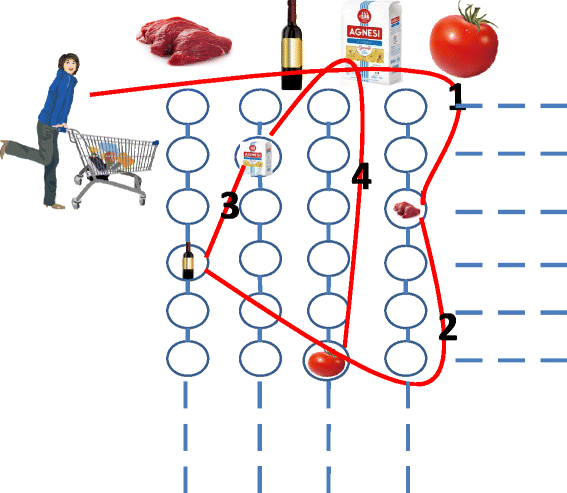
Correlations between items
-
We propose k-NN and hierarchical agglomerative clustering (HAC) algorithm to only analyze a part of the tags’ relative velocity data and mining shopping data. Compared with other shopping data mining system that need to analyze all tag information, our system reduces the amount of calculation and improves the monitoring efficiency.
-
We prototype the system by using Impinj Speedway R420 reader and passive tags to evaluate the performance of our methods. The results show that our methods can discover the popular items with an average accuracy up to 92.7% and disclose implicit correlations among items with an accuracy of 82%.

Our system can disclose the correlations among items and determine the purchase time sequence of related merchandises by a clustering algorithm.
We divide the shopping data mining procedure into two phases. In phase-I, our system discovers hot areas by k-NN machine learning algorithm. In phase-II, feedback information were used to reveal implicit relationships among items, identifying hot items and popular items by hierarchical agglomerative clustering.
The remainder of this paper is organized as follows. We overview the system in Section 2. The main designs of our system are presented in Section 3, and in Section 4, the evaluation of our scheme is exhibited. The related works are discussed in Section 5. Finally, we conclude this paper in Section 6.
2 System overview
In this section, we present four main objectives of our system, introduce signal characteristics that we used and a hardware setup, and then conduct some experiments to verify the intuitions mentioned in the introduction part.
2.1 Objectives
Our system is designed to use RSS to do deep analysis of shopping data. Specifically, it has four main objectives, namely discovering interesting items, popular items, hot areas, and related items.
-
Interesting items :Some items are often observed by customers, but are rarely purchased; we call those items interesting items. The sales history can only indicate that the product has been checkout, but can not record goods that customers are just interested in.
-
Popular items: One of the advantages of our system is that our system can identify some actions, such as holding something hovering for a while in some region and then discarded after being considered. Popular products are products that can not only attract customer interest but can also be picked for a while, no matter whether they are eventually purchased and last checkout items.
-
Correlated items: If some commodities always have similar velocity patterns, we say that these items are correlated. For example, women who want to buy a steak would also buy red wine, pasta, and tomatoes to make a romantic dinner as shown in Fig. 1; they are not adjacent, but are often purchased together, just like the real case of “beers and diapers;” in a clothes store, clothes that are frequently matched with or tried on together; in a large mall, items always in the same shopping cart, these items are considered as correlated items. Our system can disclose the correlations among items and determine the purchase time sequence of related merchandises by clustering algorithm.
-
Hot areas: The hot area is the area that most shoppers like to stroll after entering the mall, or the area where people buy things that often pass by. The dealers can optimize the layout of the store by putting the promotional items or new merchandise here.
2.2 Signal characteristics
Our system adopt velocity, which are calculated by RSS to conduct mining shopping data.
-
Received signal strength: RSS is a power indicator of the received radio signal. According to the Fris Function [8], the received radio signal power can be expressed as:
$$ P_{r}=\gamma P_{t}G_{r}^{2}G_{t}^{2}\left(\frac{\lambda}{4\pi d}\right)^{4} $$(1)where P r is the power of received backscattered signal, P t is the transmitting power by the reader, γ is the loss in the backscatter transmission, the distance between the reader antenna and the tag antenna is d, and G r is the gains of the reader antenna and G t is the gains of the tag antenna. Thus, RSS can be define as:
$$ RSS=10log\left(\frac{P_{t}}{1mW}\gamma G_{r}^{2}G_{t}^{2}\left(\frac{\lambda}{4\pi d}\right)^{4} \right) $$(2) -
Velocity of moving tags: Velocity reflects the speed of goods being moved by customers. In the shopping process, the walking speed of each customer is different; thus, we can use velocity to distinguish whether the items are moved or whether they are moved by the same customers. In the case of only RSS, how do we calculate the velocity? Our formulas are as follows :
$$ k=10log\left(\frac{P_{t}}{1mW}\gamma G_{r}^{2}G_{t}^{2}\left(\frac{\lambda}{4\pi}\right)^{4}\right) $$(3)$$ RSS=\frac{k}{\left(d+\int_{0}^{t}v\left(t \right)dt\right)^{4}} $$(4)$$ f\left(t \right)=\sqrt[4]{\frac{k}{RSS}}=\int_{0}^{t}v\left(t \right)dt+d $$(5)$$ f{}'\left(t \right)=v\left(t \right) $$(6)Compared to people’s movement speed, P t ,γ,G r , and G t can be seen as a relative fixed value; therefore, the k can be regarded as a constant, and v(t) is the velocity we ask for.
2.3 Hardware deployment
Hardware includes an Impinj Speedway reader R420 with four antennas and massive passive tags (and we also can change the amount of reader and tags according to the shopping mall size). The reader operates at 920–925 MHz UHF band and each tag reading contains a time stamp, a tag ID, and an RSSI value which are processed by a computer running in WINDOWS 7.
-
Tag and reader placement: Referring to common display modes in a large supermarket, we deployed tags in the typical scenarios that many commodities are displayed on a shelf in line. The reader is placed on the wall around the shelf or on the edge of the shelf.
-
Tag reading: Readers collect RSS by sending a RSS request to all tags within a sampling time. In order to let RSSI vectors be with the same dimensions during the time stamps for tags, mathematically, the RSS value is set to 0, if we can not receive RSSI readings of a certain tag.
2.4 Intuitions verification
In this section, we conduct many times experiments to verify the two intuitions discussed in introduction. We invite 30 volunteers to pick up goods, and reader constantly broadcasts command and collect RSS. In the beginning, we capture the RSS of tags when volunteers are just hanging out and the items are static; after that, volunteers move the items from the shelf. Readers use velocity values that are computed by RSS to draw the velocity curve. Figure 2a depicts the velocity patterns when there are no volunteers and all tags are static. The patterns of volunteers strolling around the shelf are shown in Fig. 2b, c. The figures show that when people appear in different locations, the velocity of tags will form different fluctuation pattern.

a The relative speed of the tags, when no one in the supermarket. b The relative speed of the adjacent tags that are fully covered or half blocked by volunteers, when volunteers come from nearby tags. c The relative speed of the non-adjacent tags, when customers come from the vicinity of the tags
Items which are moved by different people are depicted in Fig. 3a, b. Figure 3c plots the velocity pattern when a volunteer picks up some items to move together (tags move with the shopping cart). Those pictures show that the velocity patterns are different when items were moved by different people, but were the same when items were moved together by the same people, and when a customer takes a product from the shelf, it will interfere with the adjacent goods. Therefore, the above studies have confirmed our intuitions and shown the feasibility and potential of velocity vector for solving deep shopping data analysis problems.

a Tag C is taken away by a volunteer. b Volunteer took away tag F; after that, another customer took tag B. c A volunteer was moving with tags B and D
3 Design
We divide the shopping data mining procedure into two phases. In phase-I, our system discovers hot areas by k-NN machine learning algorithm. In phase-II, feedback information are used to reveal implicit relationships among items, identifying hot and popular items by hierarchical agglomerative clustering.
3.1 Phase-I: machine learning
During the whole process of shopping, if the customer is fond of an item, he will pick or move it for a while. Those actions will alter the items’ state from stationary to movement. Based on the above analysis, the velocity pattern would change when the status of the tag changes, which naturally separates the moved items apart from other stationary items. Namely, by observing changes in velocity values, we can identify the popular products. In real environment, however, only by the magnitude of the velocity can not exactly deduce what the state of a tag is. For example, when someone walks past a stationary tag or other tags around it are moved, this tag will have a relative speed like the velocity patterns of the six items in 4 s shown in Fig. 4, making it not easy to judge the state of the tag through a simple change of the amplitude. Although the mobile tags’ velocity pattern changes are more obvious than the stationary tags, the boundary is intangible to tell them apart. In Fig. 4, the column on the left shows the static tag’s velocity patterns, the first picture depicts the velocity patterns when there are no volunteers, the second shows the velocity patterns when volunteers stroll around the shelf, the third figure shows the fluctuating pattern of the static tag’s velocity when nearby objects have been taken. Likewise, the column on the right represents a model for moving tags. The first is that the item is picked up and turned over, and the remaining two represent the items being carried by different customers. The measurement indicates that it is possible to use k-NN classifier to divide the tags into three classes: no one near the tags (stationary tags), someone near the tags (unstable tags), and tags that were moved (mobile tags).

Velocity patterns of tags: a stationary tags and b mobile tags
We can use the number of unstable tags to find a hot area. In phase-I, our system can discover the unstable tags through machine learning, record its ID, and count the number of unstable tags, as well as the number of times to be passed by the customer. Based on the area of where each product belongs which we already know, we can determine the hot area according to the collected tag ID.
First, we need to train the mode as shown in Fig. 4 by collecting the sequence of the tags’ velocity vectors, which states are already known, then use this model to estimate the tags’ state for a given new velocity vector. Set the number of readers and reference tags as N and M respectively, then the RSS vector of the i th target tag can be defined as T i =(t(i,1),t(i,2),⋯,t(i,N)); the t(i,n) denotes the velocity of the i th target tag by the n th reader received, and n∈(1,N). And the velocity vector of the i th target tag is defined as Vt(i,n)=(vt(i,1),vt(i,2),⋯,vt(i,N)); the vt(i,n) is velocity of the i th target tag by the n th reader received. And the corresponding RSSI vector for the j th reference tag is defined as R j =(r(j,1),r(j,2),⋯,r(j,N)), and r(j,n) denotes the signal strength, and j∈(1,M). And the velocity vector of the j th reference tag is defined as Vr(j,n)=(vr(j,1),vr(j,2),⋯,vr(j,N)); the vr(j,n) is the velocity of the j th reference tag by the n th reader received.
The Euclidean distance E(i,n) between Vt(i,n) of the i th target tag and Vr(j,n) of the j th reference tag is calculated by:
Unfortunately, items are usually densely placed side by side in the supermarket shelf, and the RSS is easily affected by the multi-path effect and the change of the radiation pattern (a tag antenna’s radiation patterns will have a great impact on the adjacent tags due to mutual coupling, shielding, and reflection [9]), making the selected K, where most similar references usually do not have the same state with the target tag [10]. So, a further improvement method is proposed by [11] to mitigate the impact of the velocity fluctuation on the estimation error.
The j th reference tags’ mean value collected by the n th reader antenna is defined as u(j,n), and standard deviation is δ(j,n). Due that the target tag would have an unequal velocity when it is close to the different reference tags or is covered by an object, we use u(j,n) and δ(n,m) to optimize it. The normalized velocity of the j th reference tag n j is calculated as follows:
Hence, the revised Euclidean distance \(E_{(i, n)}^{'}\) is calculated by the following formula :
Therefore, the i th target tag has its Euclidean distance vector \(E_{(i, 1)}^{'}, E_{(i, 2)}^{'}, \cdots, E_{(i, N)}^{'}\), and the reference tag closer to the target tag is assumed to have a smaller Euclidean distance. Then, we can get the \(E_{i}^{''}\), which is the Euclidean distance vector after the revised Euclidean distances in \(E_{i}^{'}\) are sorted in an ascending order, i.e., \(E_{(i, 1)}^{''}\leq E_{(i, 2)}^{''} \leq \cdots \leq E_{(i, N)}^{''}\). The first K reference tags are the nearest neighbors (NNs) whose states are utilized to identify the state of the target tag. The weighting factor for each selected reference tag are:
where k∈(1,K). The estimated state of the i th target, i.e., y th is given by
where y k denotes the state of the k th selected reference tag. After this process, we reduce the amount of data which need to be computed by the reader effectively.
After phase-I, we can separate the moving items from all the items. In phase-II, the reader only needs to deal with the information of moving items, greatly improving the time efficiency and reducing the amount of computation.
3.2 Phase-II: hierarchical agglomerative clustering
In the clustering phase, our system first explores the velocity to discover correlated items, which are usually tried on or buy together, e.g., when people buys pasta, they also want to buy tomato, and if they need a dress, they also consider about the high-heeled shoes. Previous effort [4] proposed an RSS-based localization technique for correlated item discovery, based on an intuition that correlated items held by the same person should be in close proximity. However, this method is not accurate after applying in real-world applications since items around the customer are also very close, then they may be taken as the correlated items mistakenly. When different commodities are continuously picked up, rather than pick up simultaneously to compare, this method also does not work well.
Our system uses the observation that correlated items, either in the hands of a single customer or in the same shopping bag, once they follow a similar moving pattern with the customer, they would have the same velocity time curve. So, we can use hierarchical agglomerative clustering approach to organize tags in different groups, making the correlated items be aggregated into one group.
Since we do not know the number of target items to be tracked (new items may be added to the shopping cart or some previous items are discard by customers at any time, and we also do not know the number of customers), clustering algorithms, such as k-means [12], in which the number of clusters must be known as a priori, thus leading to this kind of clustering algorithm that can not be applied. For this reason, we adopt hierarchical agglomerative clustering (HAC) algorithm [13] to solve the challenge.
We define K as the set of velocity of the mobile tags that are identified in the phase-I, and we divide the velocity into N segments. Each segment of data is considered as a vector. Each tag i∈K has velocity vectors v i . In the HAC algorithm, each vector is initially considered as an independent cluster. At each iteration, the two similarities clusters are merged. The distance between two clusters, S i ∈K and S j ∈K, is measured with the average distance \(\bar {d}\):
where t denotes the t th segment of relative data and i, j are tag’s identifiers.
The iterations terminate when the minimum of the average speed similarity among the clusters is larger than a threshold T c , which determines the classification accuracy and time efficiency, (i.e., time delay for low values of T c , and low correct rate for high values of T c ). The optimal value of T c used in the experiments was derived experimentally (see Section 5).
We use the example of Fig. 5 to explain our algorithm. At first, each tag is considered as one individual cluster. According to Eq. 12, we can calculate the similarity of velocity vector v i based on the measured data. The results are shown in Fig. 7. The smaller the distance \(\bar {d}\) is, the more similar the two tags are. We put items into one cluster, where distance values are lower than the threshold. Hence, beer and nappies are clustered after several iteration. When there is no \(\bar {d}\) or \(\bar {d}\) is lower than the threshold T c , or only one cluster is left in the end, the iterative algorithm will be terminated, and each cluster is defined as the tags that are selected by the same person. However, there is another situation, like the lipstick in Fig. 5, which is divided into a single category. Maybe it was just being picked up at a certain time and not being put into the shopping cart, it was just a hot item. So all commodities like the lipstick should have a calculated distance \(\bar {d}\) again with the static goods, if the \(\bar {d}\) is lower than the threshold T c in the time period, it will be considered as a hot item, and the popular items are those mobile items that are identified in the phase-I minus the hot items identified in phase-II.

Disclosing implicit correlations
In the clustering process, different time segment classification results may be different, a certain group of goods may increase or decrease in the next period of time, corresponding to the product that is newly added to the shopping cart or abandoned during the process of shopping. Thus, we have the shopping order in time series, which is beneficial for retailers in optimizing the pattern of commodity display.
4 Experiments
In this section, we present the prototype implementation of our system and evaluate its performance by conducting comprehensive experiments.
Experiment hardware include multiple readers (Impinj Speedway, reader R420 every reader can connect four antenna, the antenna on shelves) at one end and a large number of passive tags (all labels on goods side). The reader works in 920–925 MHz UHF frequency band, and the system runs in the Windows 7 computer. Referring to common display modes in stores, our experiments in the typical scenarios of many commodities are displayed on a shelf in line.
4.1 Evaluation of k-NN algorithm
In our experiments, we should first determine the optimal number of NNs for the k-NN algorithm. Figure 6 shows the estimation error rate under the given number of target tags and volunteers. The estimation error decreases first and then increases with the growth of the number of NNs. The system has the minimum estimation error of 8% when K=7. The seven NNs are optimal in these measurements. and therefore, it is adopted in the following measurements here.

Estimation error rate under different reference NNs

a Classification error rate under a different number of target goods. b Classification error rate under a different number of customers
Then, we identify the tags which have been moved by the k-NN algorithm and compare it with the ground truth. Figure 7a compares the k-NN algorithm under different numbers of targets in each shopping cart. The estimation error rates of the k-NN algorithm are not changed basically. And Fig. 7b compares the k-NN algorithm under different numbers of customers. The estimation error of the k-NN algorithm increases significantly from 8.5 to 11.5% when customers from 10 to 25 due to high RSS variance led by severe people interaction. Its estimation error then slowly increases for more than 25 customers, which can prove that our algorithm is robust to the number of customers and can be used in large shopping malls.
Next, we verify the accuracy of the identification of hot areas. Before the start of the experiment, we first make a distinction between all the passages. Figure 8 shows the result of use k-NN algorithm to speculate hot areas. The vertical coordinate is the sum of unstable items number (assuming that the number of unstable commodities is n, where the number of instability of product i is t i , then we set the sum of the unstable goods number is (t1+t2+⋯+t i +t n )). From the experiment results, we can learn that aisle 1 is a hot area that we want to find, and our approach is feasible to accurately find the area of large people flow.

Number of unstable tags in each aisle
4.2 Evaluation of HAC algorithm
It is crucial to tune the parameter of threshold T c for performance of HAC algorithm. T c determines the analysis accuracy of the system, and it is also related to the processing time. So, we first determine the T c , then adopt this threshold to estimate the following measurements. As shown in Fig. 9, the system has the minimum estimation error of 81% when T c = 4. When the threshold is higher or lower than 4, the error rate will increase. This is because when the threshold is too high, items with no correlation are divided into a group. And when the threshold is too low, correlated items can not be divided into a group.

Estimation error rate under different T c
Next, we evaluate the performance of HAC algorithm to identify the correlated, hot, and popular items under different numbers of items in each shopping cart and under different numbers of customers. We arrange 30 volunteers to take any number of items to do the experiments for 50 times, and the number of volunteers in each trial is the same. We show the error rate in Fig. 10a. When items in the shopping cart are from one to three, the increase of estimation error is not very obvious, but when we have more than three items, the error rate increase rapidly due to high RSS variance led by items’ interaction. Its estimation error then increases slightly for more than seven targets. Figure 10b shows the error rate in the case of different numbers of customers. As we can see, our system can find those items even the volunteers are more than 20.

a Clustering error rate under a different number of target goods. b Clustering error rate under a different number of customers
Figure 11 shows the accuracy of our system to find the order of goods being bought by different customers. We let 30 volunteers go into the mall and select different quantities of items in the fixed order. The experiment is conducted 50 times, then we use our method to estimate the orders, the accuracy decreases slightly with the increase of the number of items and the number of volunteers. Specifically, the error rate obviously increases when the number of target tags increases due to some items are added to the shopping cart over a short period of time, and we can not make a distinction between the order of goods. When the number of customers are small, the detection accuracy is around 97.8%, whereas the performance gets worse with more volunteers. This may because the correlated items are assigned to the wrong group.

a Clustering error rate under a different number of target goods. b Clustering error rate under different number of customers
4.3 Evaluation of time efficiency
Mining shopping data is useful, since the information can contribute to a better program for retailers so as to improve sales. It is important to improve time efficiency in real shopping environment mainly due to two reasons. One the one hand, in large shopping malls where there are a lot of goods, if you want to deal with the data of all commodities, the amounts of data are very large, which will result in time delay. On the other hand, customers may just pick up an item from a shelf, then put it down, and the duration is short for data collection. Therefore, our system introduces k-NN to solve this problem. To validate the efficiency, we compare it with a system where we do not use the k-NN algorithm to preprocess.
Figure 12 is the comparison of computing time between k-NN and non-k-NN, where we assume the goods that are moved make up 5% of all the goods. From the results, when the number of moving tags is above 100, k-NN algorithm has 25% or more time saved than non-k-NN with N ranging from 1 to 6000. That is because the use of k-NN algorithm can effectively reduce the number of tags to be processed in the second phase.

Comparison of time efficiency
5 Related work
Sales history is an important source for customer behavior analysis. However, it only reflects the items purchased by customers and misses other customer behaviors [14]. Compared to in-store shopping, online shopping [15] is where it is easier to complete this task. Online shoppers’ behaviors, such as clicks, price comparisons, and search records, all those can be captured by the Web. For physical stores, capturing the customers’ behavior is extremely difficult. So, deploying the data collection device in a shopping cart was proposed in [16], in which portable devices are deployed on shopping carts to collect data. Some works for physical stores focus on other kinds of data, such as in [17], You et al. adopt shopping time, and Fujino et al. take advantage of shopping paths of customers in [18]. In [19], Niu et al. present a framework for detecting and recognizing human activities on simple statistics compiled on tracked trajectories. Rallapalli et al. track each of physical browsing by users using a combination of a first person vision enabled by smart glasses and inertial sensing using both the glasses and a smartphone [20], while others use RFID systems in stores to collect customer data comprehensively. In [21], the describe development for RFID-based personal shopping assistant system for retail stores, and the authors in [22] present a case study of an RFID project at Galeria Kaufhof. In addition, in [23], the authors develop a customized commodity recommendation algorithm and a shopping route determination and guiding algorithm. CBID [4] adopts a Doppler effect-based protocol to detect tag movements. Tagbooth [5] leverages physical-layer information to exploit the motion of tagged commodities by phase and RSS to recognize customers actions. ShopMiner [6] harnesses the distinct yet stable patterns of phase in the time series when customers move their desired items to detect comprehensive shopping behaviors. Our work use RFID systems in stores to collect customer data, but ours differs from these three works. On the one hand, our system incorporates four key factors that are essential to retailers, i.e., which items only attracted the interest of customers, which items are purchased by most customers, which items they match with, which region has a large number of people, and what is the general order of goods being bought by customers. In contrast, CBID, Tagbooth, and ShopMiner only include two or three important factors. On the other hand, our system solely adopts the RSS in mining customer shopping behavior, whereas CBID, Tagbooth, and ShopMiner mainly rely on RSSI, Doppler shift, and phase for customer behavior identification.
6 Conclusions
In this paper, we propose to explore the received signal strength of passive RFID tags to achieve shopping data mining. Based on the velocity is different when items are in different states or carried by different customers, we leverage machine learning and hierarchical agglomerative clustering to carry out in-depth analysis of velocity data and achieve popular and hot items identification, find the correlation between items, and find the general order of goods being purchased. We have built the proof-of-concept system and conducted extensive experiments to test the performance of our system. Our evaluations show a very good performance.
References
D Preuveneers, Y Berbers, Internet of things: A context-awareness perspective. The Internet of Things: From RFID to the Next-Generation Pervasive Networked Systems, 287–307 (2008).
Y Zheng, M Li, P-mti: physical-layer missing tag identification via compressive sensing. IEEE/ACM Trans. Netw. (TON). 23(4), 1356–1366 (2015).
T Liu, L Yang, Q Lin, Y Guo, Liu Y, et al, in Proceedings - IEEE INFOCOM. Anchor-free backscatter positioning for rfid tags with high accuracy (IEEE, 2014), pp. 379–387.
J Han, H Ding, C Qian, D Ma, W Xi, Z Wang, Z Jiang, Shangguan L. Cbid: a customer behavior identification system using passive tags (IEEE, 2014), pp. 47–58.
T Liu, L Yang, X-Y Li, H Huang, Liu Y, et al, in Computer Communications (INFOCOM), 2015 IEEE Conference on. Tagbooth: deep shopping data acquisition powered by rfid tags (IEEE, 2015), pp. 1670–1678.
L Shangguan, Z Zhou, X Zheng, et al, in Proceedings of the 13th ACM Conference on Embedded Networked Sensor Systems. Shopminer: mining customer shopping behavior in physical clothing stores with cots rfid devices (ACM, 2015), pp. 113–125.
W Ruan, L Yao, QZ Sheng, et al, in Proceedings of the 11th international conference on mobile and ubiquitous systems: computing, networking and services. ICST (Institute for Computer Sciences, Social-Informatics and Telecommunications Engineering). Tagtrack: device-free localization and tracking using passive RFID tags, (2014), pp. 80–89.
DM Dobkin, The rf in RFID: uhf RFID in practice (Newnes, 2012).
F Lu, XS Chen, TY Terry, in IEEE International Conference on Rfid. Performance analysis of stacked RFID tags (IEEE, 2009), pp. 330–337.
XF Li, LY Xi, Y Huang, RFID-based localization and tracking technologies. IEEE Wireless Commun. 18(2), 45–51 (2011).
Z Zhang, Z Lu, V Saakian, X Qin, Q Chen, LR Zhen, Item-level indoor localization with passive UHF RFID based on tag interaction analysis. IEEE Trans. Ind. Electron. 61(4), 2122–2135 (2014).
J Macqueen, in Proceedings of the fifth Berkeley symposium on mathematical statistics and probability. Some methods for classification and analysis of multivariate observations, (1967), pp. 281–297.
J Franklin, The elements of statistical learning: data mining, inference and prediction. The Mathematical Intelligencer. 27(2), 83–85 (2005).
A Ainslie, PE Rossi, Similarities in choice behavior across product categories. Marketing Sci. 17(2), 91–106 (1998).
J Wang, Y Zhang, in Proceedings of the 36th international ACM SIGIR conference on Research and development in information retrieval. Opportunity model for e-commerce recommendation: right product; right time (ACM, 2013), pp. 303–312.
TP O’Hagan, CE Lewis, Shopping cart mounted portable data collection device with tethered dataform reader: U.S. Patent 5,821,513. 1998-10-13.
CW You, CC Wei, YL Chen, HH Chu, MS Chen, Using mobile phones to monitor shopping time at physical stores. IEEE Pervasive Comput. 10(2), 37–43 (2011).
T Fujino, M Kitazawa, T Yamada, M Takahashi, G Yamamoto, A Yoshikawa, T Terano, Analyzingin-store shopping paths from indirect observation with RFID tags communication data. J. Innov. Sustainability RISUS ISSN 2179-3565. 5(1), 88–96 (2014).
W Niu, J Long, et al, in Multimedia and Expo, 2004. ICME ’04 2004. IEEE International Conference on. Human activity detection and recognition for video surveillance. Vol.1 (IEEE, 2004), pp. 719–722.
S Rallapalli, A Ganesan, K Chintalapudi, VN Padmanabhan, L Qiu, et al, in Proceedings of the 20th annual international conference on mobile computing and networking. Enabling physical analytics in retail stores using smart glasses (ACM, 2014), pp. 115–126.
EWT Ngai, KKL Moon, JNK Liu, KF Tsang, R Law, FFC Suk, ICL Wong, et al, Extending crm in the retail industry: an rfid-based personal shopping assistant system (Communications of the Association for Information Systems, 2008). 23(1):16.
F Thiesse, J Alkassab, E Fleisch, Understanding the value of integrated rfid systems: a case study from apparel retail. Eur. J. Inf. Syst. 18(6), 1–23 (2009).
JL Hou, TG Chen, An RFID-based shopping service system for retailers. Adv. Eng. Inf. 25(1), 103–115 (2011).
Funding
The paper is supported by The National High Technology Research and Development Program (“863” Program) of China (2015AA016901):High linearity laser diode array and high saturation power photodiode array; The General Object of National Natural Science Foundation under Grants (61572346): The Key Technology to Precisely Identify Massive Tags RFID System With Less Delay; The General Object of National Natural Science Foundation(61772358): Research on the key technology of BDS precision positioning in complex landform; the International Cooperation Project of Shanxi Province under a grant (No. 201603D421012): Research on the key technology of GNSS area strengthen information extraction based on crowd sensing; and The General Object of National Natural Science Foundation under a grant (No. 61572347): Resource Optimization in Large-scale Mobile Crowdsensing: Theory and Technology.
Availability of data and materials
Not applicable.
Author information
Authors and Affiliations
Contributions
JZ and DL conceived and designed the study. LW performed the experiments and participated in the paper writing. YL revised the manuscript and took charge of the all the work of paper submission. BY gave some proposal for the experiments. BZ and RB reviewed and revised the manuscript. All authors read and approved the final manuscript.
Corresponding author
Ethics declarations
Competing interests
The authors declare that they have no competing interests.
Publisher’s Note
Springer Nature remains neutral with regard to jurisdictional claims in published maps and institutional affiliations.
Rights and permissions
Open Access This article is distributed under the terms of the Creative Commons Attribution 4.0 International License(http://creativecommons.org/licenses/by/4.0/), which permits unrestricted use, distribution, and reproduction in any medium, provided you give appropriate credit to the original author(s) and the source, provide a link to the Creative Commons license, and indicate if changes were made.
About this article

Cite this article
Zhao, J., Wang, L., Li, Da. et al. Mining shopping data with passive tags via velocity analysis. J Wireless Com Network 2018, 28 (2018). https://doi.org/10.1186/s13638-018-1033-5
Received:
Accepted:
Published:
DOI: https://doi.org/10.1186/s13638-018-1033-5