- Research
- Open access
- Published:
Performance analysis of feedback-free collision resolution NDMA protocol
EURASIP Journal on Wireless Communications and Networking volume 2018, Article number: 45 (2018)
Abstract
To support communications of a large number of deployed devices while guaranteeing limited signaling load, low energy consumption, and high reliability, future cellular systems require efficient random access protocols. However, how to address the collision resolution at the receiver is still the main bottleneck of these protocols. The network-assisted diversity multiple access (NDMA) protocol solves the issue and attains the highest potential throughput at the cost of keeping devices active to acquire feedback and repeating transmissions until successful decoding. In contrast, another potential approach is the feedback-free NDMA (FF-NDMA) protocol, in which devices do repeat packets in a pre-defined number of consecutive time slots without waiting for feedback associated with repetitions. Here, we investigate the FF-NDMA protocol from a cellular network perspective in order to elucidate under what circumstances this scheme is more energy efficient than NDMA. We characterize analytically the FF-NDMA protocol along with the multipacket reception model and a finite Markov chain. Analytic expressions for throughput, delay, capture probability, energy, and energy efficiency are derived. Then, clues for system design are established according to the different trade-offs studied. Simulation results show that FF-NDMA is more energy efficient than classical NDMA and HARQ-NDMA at low signal-to-noise ratio (SNR) and at medium SNR when the load increases.
1 Introduction
The fifth generation (5G) of cellular networks, set for availability around 2020, is expected to enable a fully mobile and connected society, characterized by a massive growth in connectivity and an increased density and volume of traffic. Hence, a wide range of requirements arise, such as scalability, rapid programmability, high capacity, security, reliability, availability, low latency, and long-life battery for devices [1]. All these requirements pave the way for machine-type communications (MTC), which enable the implementation of the Internet of Things (IoT) [2]. Unlike typical human-to-human communications, MTC devices are equipped with batteries of finite lifetime and generate bursty and automatic data without or with low human intervention, so that traffic in the uplink direction is accentuated [3]. MTC systems consider different use cases that range from massive MTC, where the number of deployed devices is very high, to mission-critical MTC, where real-time and high-reliability communication needs have to be satisfied [4].
To address such a massive number of low-powered devices generating bursty traffic with low latency requirements, simple medium access control (MAC)-layer random access protocols of ALOHA-type are preferred because they offer a relatively straightforward implementation and can accommodate bursty devices in a shared communication channel [4, 5]. They are indeed used in today’s most advanced cellular networks (as the random access channel (RACH) in LTE) [6] and are being considered in different MTC systems, such as LoRa [7], SigFox, enhanced MTC [8], narrowband (NB) LTE-M [9, 10], and NB-IoT [11–13].
Basic ALOHA-type protocols are based on the collision model: a packet is received error-free only when a single device transmits. Thus, the MAC layer and the physical (PHY) layer are fully decoupled. In [14], Guez et al. made a fundamental change in the collision model and introduced the multipacket reception (MPR) model: when there are simultaneous transmissions, instead of associating collisions with deterministic failures, reception is described by conditional probabilities. Therefore, signal processing techniques enable a receiver to decode simultaneous signals from different devices and hence collisions can be resolved at the PHY layer. As a result, a tighter interaction between PHY and MAC layers is achieved [14–16].
MPR can be realized through many techniques, which are classified according to three different perspectives: transmitter, trans-receiver, and receiver (see [17] for details). Among all of them, a promising trans-receiver approach based on random access for different 5G services is the network-assisted diversity multiple access (NDMA) protocol. NDMA was initially presented in [18] for flat-fading channels and, afterwards, extended to multi-path time-dispersive channels in [19]. The basic idea of NDMA is that the signals received in collided transmissions are stored in memory and then they are combined with future repetitions at the receiver so as to extract all collided packets with a linear detector. In the single-antenna case and under the assumption of perfect reception, NDMA only requires the number of repetitions to be equal to the number of collided packets [18]. Thus, NDMA dramatically enhances throughput and delay performance as compared to ALOHA-type protocols, but estimation of the number of devices involved in a collision (e.g., P devices) and a properly adjustment of the number of repetitions (i.e. P−1) is required every time a collision occurs.
Many NDMA protocols, and variations of it, have been proposed and analyzed in the literature, including different ways to determine the number of devices involved in a collision [18–22], interference cancellation receivers [23–25], and modified protocols that use channel knowledge at the transmitter side [26, 27]. Stability analysis of NDMA was addressed in [28–30]. Finally, the hybrid automatic repeat request (HARQ) concept was applied to NDMA in [31] (named H-NDMA) in order to deal with reception errors at low/medium SNR by forcing devices involved in a collision of P devices to transmit repetitions more than P−1 times. This way, packet reception was significantly improved at low SNR with H-NDMA as compared to classical NDMA.
One of the main drawbacks of NDMA protocols is, however, the overhead required to identify collisions and adjust the number of repetitions accordingly every time a collision occurs (which implies communicating it to all the devices involved in the collision) [18]. Indeed, devices need to decode control signaling at every time slot to know if the subsequent time slot is reserved for repetitions or not, hence increasing the energy consumption. This aspect is critical for MTC devices with finite battery lifetime.
To cope with these issues, authors in [32] proposed a non-centralized procedure for NDMA, coined feedback-free NDMA (FF-NDMA), in which the number of time slots for repetitions is kept constant to R (conforming a contention period (CP)) and is equal for all devices and transmissions. See Fig. 1 for R = 3. Accordingly, devices are only allowed to start transmission at the beginning of the CP and will do so R times. This way, collisions of up to R devices can be resolved in the single-antenna case without requiring the receiver to communicate the collision multiplicity to the devices every time a collision occurs and avoiding the signaling related to the state (reserved for repetitions or not) of the subsequent time slot. The joint PHY-MAC performance analysis of FF-NDMA protocol was performed in [33] for the general case of MIMO systemsFootnote 1 with orthogonal space-time block coding (OSTBC). Significant throughput and energy gains as compared to ALOHA-based schemes were reported with a non-centralized protocol that requires low overhead. Nevertheless, it was assumed in [32, 33] that whenever a packet was received in error at the receiver then said packet was lost, since FF-NDMA was initially designed to address the broadcast protocol in ad hoc networks where no feedback is available.
Although NDMA and FF-NDMA were initially proposed a decade ago, the emerging MTC systems (with different requirements than those of conventional human-based cellular networks) suggest reviewing random access protocols with MPR and analyzing its applicability to the uplink communication in cellular networks [3], specially for scenarios characterized by a large number of devices, limited signaling load, low energy consumption, and high reliability. In particular, NDMA-based protocols are highly attractive for massive MTC. NDMA has been deeply analyzed in the recent literature with different protocols (e.g., H-NDMA [31]). However, FF-NDMA misses such wide analysis while it is suitable for massive MTC scenarios due to its low associated signaling load and reduced implementation complexity. Indeed, it is worth mentioning that NB-IoT [11] and the new radio (NR) access technology design for 3GPP 5G systems [34] already consider a contention-based transmission mode with a predefined number of packet repetitions (known as uplink grant-free access, in which devices contend for resources, and multiple predefined repetitions are allowed, as specified in [34]). Such uplink grant free access in NR targets at least for massive MTC and would allow the implementation of FF-NDMA.
In this paper, we analyze the FF-NDMA protocol with MIMO configurations and OSTBC from a cellular network perspective, in which multiple devices intend to communicate with a base station (BS), as shown in Fig. 1. The MIMO system defined and analyzed in the sequel carries over to a multi-cell scenario where cell-edge terminals experience similar average SNR to an x-number of BSs that are able to receive and decode packets in a distributed way with an x-fold number of received antennas. Differently from [32, 33], in which no feedback was considered and whenever a packet was received in error then the packet was discarded, we use a general model in which packets are not discarded. To do so, we consider a finite-user slotted random access system where devices can be either transmitting, thinking (i.e., there is no packet to transmit), decoding, or backlogged (i.e., packet transmission was erroneous and the device is waiting for a new transmission opportunity) and we assume that each device is equipped with a single-packet bufferFootnote 2. Therefore, FF-NDMA is feedback-free in the sense that it is not needed to broadcast information related to the number of repetitions and to the state of the forthcoming time slots (as in NDMA or H-NDMA) but, in contrast to [32, 33], ACK feedback to acknowledge a correct detection of the devices’ packets per CP is assumed.
In this context, the main contributions of this paper are summarized as follows:
-
we develop a joint PHY-MAC analysis of the FF-NDMA protocol by using the MPR model and, then, characterize the system through a finite Markov chain, for which the system state probabilities and the transition probabilities among them are obtained in closed-form.
-
we characterize analytically the FF-NDMA protocol in terms of throughput, delay, capture probability (i.e., probability of a successful transmission or, equivalently, reliability of the protocol), energy, and energy efficiency (i.e., efficiency of the protocol, which is measured through a throughput-energy ratio). Also, we propose two criteria to analyze the stability of finite-user random access with single-packet bufferFootnote 3.
-
we investigate the system performance of FF-NDMA as a function of the CP length (R), for different SNR and load conditions, and we compare FF-NDMA with S-ALOHA, classical NDMA [18], and H-NDMAFootnote 4 [31]. As we will see, the energy consumption is reduced with FF-NDMA as compared to H-NDMA in certain situations due to the lower control signaling to be decoded. To address the throughput-energy trade-off, we use the energy-efficiency metric and focus on determining the circumstances in which FF-NDMA is more energy efficient than H-NDMA.
Organization: The paper is organized as follows: in Section 2, we assess the differences between FF-NDMA and other NDMA-based protocols (including NDMA and H-NDMA) and then we present the system model and the main features of the FF-NDMA protocol. Section 3 establishes the MPR model and characterizes the system by using a finite Markov chain, for which the system state probabilities (related to the backlog state) are derived. Then, in Section 4, based on the obtained system state probabilities, expressions for throughput, delay, capture probability, energy, and energy efficiency are developed and two stability conditions are set. Section 5 presents the simulation results by using different SNR and different offered loads and system design clues are extracted. Finally, conclusions are drawn in Section 6.
Notation: In this paper, scalars are denoted by italic letters. Boldface lower-case and upper-case letters denote vectors and matrices, respectively. For given real-valued scalars a and b, \(\text {Pr}\left (a {\le } b \right)\), \(\text {Pr}\left (a {=} b \right)\), \(\text {Pr}\left (a {=} b | \mathcal {C} \right)\), ⌈a⌉, and \(\log _{2} (a)\), denote the probability of a being smaller than b, the probability of a being equal to b, the probability of a being equal to b given condition \(\mathcal {C}\), the ceiling function of a, and the base 2 logarithm of a, respectively. For given positive integer scalars a and b, \(\left ({\begin {array}{c} a\\ b \end {array}} \right)\)refers to the binomial coefficient and a! denotes the factorial of a. For a given vector a, aT stands for the vector transpose. \(\mathcal {Q}(.)\) refers to the Q-function (i.e., the integral of a Gaussian density). \(\mathbb {R}^{m\times n}\), \(\mathbb {R}_{+}^{m\times n}\), and \(\mathbb {C}^{m\times n}\) denote an m by n dimensional real space, real positive space, and complex space, respectively.
2 System model
In this section, we first compare FF-NDMA protocol with classical NDMA [18] and H-NDMA [31], and then present the system model for FF-NDMA.
2.1 Comparison of NDMA protocols
Figure 2 shows the protocol differences between NDMAFootnote 5 and FF-NDMA with R=3. To perform a fair protocol comparison, we assume that each time slot contains a data part for data transmission and a control part for feedback from BS (which is not always used in FF-NDMA).
In FF-NDMA, transmissions are attempted at the CP start and the number of repetitions is fixed to the CP length (R repetitions) independently of the number of devices that collide. In contrast, in NDMA, transmissions are attempted at the time slot scale and the number of repetitions is dynamically adapted according to the number of collided packets. H-NDMA follows classical NDMA operation but, at low/medium SNR, the BS might ask for additional repetitions on a HARQ basis to improve packet reception. For these reasons, the throughput of FF-NDMA can not be as large as that of classical NDMA at high SNR and as that of H-NDMA at any SNR range. However, load signaling, implementation complexity, and energy consumption are reduced with FF-NDMA.
Under NDMA, receiving and decoding control signaling from the BS is required at every time slot for different purposes: to know if the subsequent time slot is either busy or free (i.e., reserved for repetitions of collided packets or not), to receive ACK in case a packet was transmitted, and to know the number of repetitions to be performed in case a packet was transmitted but not successfully decoded due to collision [18]. H-NDMA requires extra signaling load from the BS towards devices to request additional repetitions on a HARQ basis [31], once the repetitions of NDMA have been completed. On the other hand, in FF-NDMA, control signaling is only needed to receive ACK at those CPs in which a packet was transmitted. This makes the application of FF-NDMA to MTC systems highly attractive because the energy consumption for control signaling decoding is reduced. The difference in the control signaling to be decoded with FF-NDMA and NDMA is illustrated in Fig. 2 in orange color.
To summarize, the throughput of FF-NDMA is going to be lower than the throughput of H-NDMA, but the energy consumption can be reduced with FF-NDMA. In this line, in Section 5.2, we use the energy efficiency as a suitable metric to address the throughput-energy trade-offs between FF-NDMA and H-NDMA and, hence, determine which protocol is more energy efficient under different circumstances.
In addition, due to the lower control signaling to be decoded with FF-NDMA, its implementation complexity is also significantly reduced as compared to NDMA or H-NDMA, because devices do not need to decode control signaling from the BS at every time slot and can enter into sleep mode. With FF-NDMA, decoding of a single-control signaling per CP in which transmission was attempted is required. With NDMA or H-NDMA, decoding of control signaling at every time slot while data is in the buffer is needed to know if transmission can be attempted and to get the feedback.
Finally, it is important to emphasize that NDMA and H-NDMA require a self-contained time slot, as shown in Fig. 2, in which the feedback for repetitions is received just after the packet transmission and devices can attempt a repetition at the subsequent time slot. However, conventional repetitions processes (e.g., HARQ) might take some time slots between obtaining the feedback and retransmitting again [35]. In this situation, FF-NDMA avoids the additional delay that appears in NDMA and H-NDMA under non-ideal repetition processes owing to the fact that FF-NDMA does not rely on feedback to perform repetitions. Both the energy savings (due to lower control signaling to decode) and the delay reductions (under non-ideal repetition processes) are evaluated in Section 5.1.
2.2 System model for FF-NDMA
Consider a wireless cellular system composed of one BS with N receive antennas and a deployment of K devices that will transmit packets to the BS through a slotted random access network, as shown in Fig. 1. Every device is equipped with M transmit antennas and has a single-packet buffer.
A frame composed of time slots is adopted. Each time slot contains a data part for data transmission from devices to BS and a control part for feedback from BS to devices (which is not always used), see Fig. 2. Time slots are grouped into contention periods (CPs) of R time slots. We assume that each device is CP- and slot-synchronous with the BS. Devices transmit whenever they have a packet in their buffer at the beginning of the CP, and packet repetitions are performed during the CP, so that devices transmit their packets R times using the data plane. After the R repetitions, the BS acknowledges reception of the correctly received packets through the control channel, so that devices known if transmission was successful or not. Note that the maximum number of packets that can be simultaneously decoded at a BS with N antennas and R repetitions is \(\tilde {R} = NR\).
In this scenario, collisions come up and every device can be in one of four different device states: thinking, transmitting, decoding, or backlogged. The device state diagram is shown in Fig. 3. In the thinking state, the device does not have a packet in its buffer and does not participate in any scheduling activity. In this device state, a device generates a packet with probability σ. Once a packet is generated, its transmission is attempted at the beginning of the next CP and repeated during R time slots (which corresponds to the transmitting state). After transmission, the device decodes an acknowledgment of receipt message from the BS. If the transmission succeeds (i.e., ACK feedback is received), the device remains in the thinking state. Otherwise, the device moves into the backlogged state and retransmits the packet with probability υ. When the packet is finally successfully decoded at the BS, the device moves back to the thinking state and the process restarts again.

State diagram of the device operation
We follow classical NDMA [18] and H-NDMA [31] assumption that uniform average power from every device is received at the BS. This is possible thanks to the uplink slow power control mechanism [36]. Accordingly, all devices are received at the BS with the same average SNR (γ). The use of uplink power control has the benefit that the scenario is terminal-wise symmetric (in terms of average SNR) and the MPR model can be thus applied, as it will be shown in Section 3.
2.2.1 Signal model
To exploit transmit diversity with no channel knowledge at the terminal sideFootnote 6, transmission of each device is done through an OSTBC with Q complex symbols that are spread in time and space over T channel uses and M transmit antennas. Therefore, the transmitted signal matrix for the kth device, \(\mathbf {X}_{k}{\in }\mathbb {C}^{M\times T}\), is expressed as [37]
where αk,q and βk,q refer to the real and imaginary parts of the qth complex symbol at the kth device, respectively, and \(\mathbf {A}_{q},\mathbf {B}_{q} \in \mathbb {R}^{M\times T}\) denote the pair of real-valued code matrices that define the OSTBC [38]. We assume that the transmitted symbols are m-QAMFootnote 7.
Considering a flat fading channel constant over the time slot and that \(\tilde {k}\) devices are transmitting, the received signal at the N antennas of the BS over T channel uses in the rth time slot, \(\mathbf {Y}_{r}{\in }\mathbb {C}^{N\times T}\), is given by [39]
where P k stands for the transmitted power of the kth device, L k refers to the slow propagation losses (including pathloss and shadowing) between the kth device and the BS, \(\mathbf {H}_{k,r}{\in }\mathbb {C}^{N\times M}\) is the Rayleigh flat-fading channel matrix between the antennas at the kth device and the BS during the rth time slot that contains zero mean complex Gaussian components, and \(\mathbf {W}_{r}{\in }\mathbb {C}^{N\times T}\) denotes the received noise that is composed of zero mean complex Gaussian components with variance \(\sigma _{\mathrm {w}}^{2}\). The average received SNR is given by \(\gamma {=}\frac {P_{k}}{L_{k}\sigma _{\mathrm {w}}^{2}}\) and is uniform among devices due to the uplink slow power control mechanism (which adjusts the uplink power P k according to the slow propagation losses L k at every device).
The BS combines the received signals in a CP of R time slots to perform multi-user detection. We assume that the channel is constant on one time slot but uncorrelated between time slots (fast-fading channel assumption)Footnote 8. Accordingly, assuming that \(\tilde {k}\) devices are present, the received signal in a CP can be arranged in vector form by separating the real and imaginary parts as (see [37], Section 7.1):
where \(\mathbf {y}_{r}{\in }\mathbb {R}^{2NT\times 1}\) and \(\mathbf {w}_{r}{\in }\mathbb {R}^{2NT\times 1}\) contain the real and imaginary parts of the received signal and the noise samples in the rth time slot (see (2)), \(\mathbf {x}_{k}=[\alpha _{k,1}\dots \alpha _{k,Q} \ \beta _{k,1}\dots \beta _{k,Q}]^{T}{\in }\mathbb {R}^{2Q\times 1}\) contains the 2Q real and imaginary parts of the complex symbols transmitted by the kth device (see (1)), and \(\bar {\mathbf {H}}_{k,r}{\in }\mathbb {R}^{2NT\times 2Q}\) denotes the equivalent channel matrix for the kth device during the rth time slot. The equivalent channel matrix \(\bar {\mathbf {H}}_{k,r}\) depends on the Rayleigh flat-fading channel matrix (Hk,r in (2)) and the pair of real-valued code matrices (A q ,B q in (1)) (see details in [33], Appendix). According to this, \(\mathbf {y},\mathbf {w}{\in }\mathbb {R}^{2NTR\times 1}\), \(\mathbf {x}{\in }\mathbb {R}^{2Q\tilde {k}\times 1}\), and \(\bar {\mathbf {H}}{\in }\mathbb {R}^{2NTR\times 2Q\tilde {k}}\).
Note that to perform decoding of the contending signals, the receiver (BS) has to get the identity of the contending devices to estimate the channel matrices from them. In this regard, we assume that all devices have orthogonal pilot signals and that channels are perfectly acquired at the receiver side. The effect of a limited number of orthogonal pilot signals, non-orthogonal pilot signals, and imperfectly acquired channels is out of the scope of the paper and is left as interesting future work.
2.2.2 Packet error rate
By using a decorrelating receiver at the BS that combines the repetitions of devices attempting transmission within a CP of R time slots (see (3)), the multiple access interference is vanished and the bit error rate (BER) is invariant to the amplitudes of the interfering signals [33]. Therefore, for m-QAM, the BER of device k given that \(\tilde {k}\) devices are transmitting is given by [40, 41]
where \(\mathcal {Q}(.)\) refers to the Q-function (the integral of a Gaussian density) and \(\chi _{\tilde {k},k}\) is a chi-square distributed random variable with \(\text {dof}_{\tilde {k}}\) degrees of freedom for any OSTBC with M=T:
For 4-QAM (QPSK), the BER expression in (4) is reduced to \(\text {BER}_{\tilde {k},k}{=}\mathcal {Q}\left (\sqrt {\frac {\chi _{\tilde {k},k}\gamma }{2M}}\right)\). In case that m-PSK was considered, the BER expression in (4) should be modified according to [40] and the whole forthcoming analysis would apply as well.
In (4), we have assumed fixed power spent at devices per time slot. This will allow us to compare the FF-NDMA protocol with classical NDMA [18] and H-NDMA [31], in which constant power per time slot is used since devices do not know the number of repetitions to be performed until a collision occurs and the BS communicates so.
Note that while R is a value to be fixed by the network, the value of \(\tilde {k}\) is random in each CP and depends on K, σ, and υ. So, the BER in a CP depends not only on the average SNR (γ) but also on the actual number of devices that are transmitting (\(\tilde {k}\)).
As in [33], we assume that a packet is in error whenever the BER in (4) is above a certain threshold ω. Therefore, an upper bound of the packet error rate (PER) for device k given that \(\tilde {k}\) devices are transmitting can be found as \(\text {PER}_{\tilde {k},k}{\le }\text {Pr}(\text {BER}_{\tilde {k},k}{\ge } \omega)\). According to this and (4), we get
which can be computed according to the cumulative function of the chi distribution in closed-form as
where
It is important to recall that, as γ is equal for all devices, distinction among specific devices is not necessary and the following condition is fulfilled (see (7)):
3 Markov model for FF-NDMA
Analytic characterization of the performance and stability of the FF-NDMA protocol with MPR requires the use of a Markov model that incorporates different states of the system and the transition probabilities between them. In this regard, in this section we first set up the MPR model for the FF-NDMA protocol, which will allow us to work with conditional probabilities instead of associating collisions or erroneous receptions with deterministic failures. Then, according to the MPR model, we derive analytic expressions for the system state probabilities of the finite Markov chain that represents the FF-NDMA protocol.
3.1 MPR matrix
The MPR model is characterized by an MPR matrix that contains conditional probabilities, see [14]. Under FF-NDMA, the MPR matrix \(\mathbf {C} {\in } \mathbb {R}_{+}^{\tilde {R} \times (\tilde {R}+1)}\) with \(\tilde {R}~{=}~NR\) is given by
where Cx,y, \(1 {\le } x {\le } \tilde {R}\), and 0≤y≤x denotes the probability that, given x transmitting devices, y out of x transmissions are successful. The number of non-zero rows of the MPR matrix is given by the maximum number of packets that can be simultaneously decoded, i.e., \(\tilde {R}\).
As γ is assumed equal for all K devices, we do not need to distinguish among specific devices so that the element Cx,y of the MPR matrix C contains the product of PERs corresponding to the combinations of x devices for which y transmissions are successful and x−y are not. According to (9), the elements of the MPR matrix in (10) (i.e., Cx,y for \(1 {\le } x {\le } \tilde {R}\), 0≤y≤x) are given by
and Cx,y=0 for y>x. Thus, we can complete the MPR matrix that characterizes the FF-NDMA protocol, C in (10), using (7), (9), and (11).
3.2 Markov chain for the system states
Let random variable B(s) denote the number of backlogged devices at the beginning of CP s. B(s) is referred to as the system state, which depends on the previous system state (i.e., B(s−1)) as well as on the number of devices whose state has changed during CP s. Hence, the process can be modeled by a finite Markov chain since B(s)≤K. Figure 4 shows the Markov chain for a simplified scenario with K = 3.

Markov chain of the system state (number of backlogged devices) in FF-NDMA protocol for K=3
The steady-state probability of the system being in state i (π i ) is thus given by
and the transition probability from system state i to j (p ij ,0≤i,j≤K) is defined as [42]
Notice that, under conventional slotted ALOHA, downward transitions are only possible from system state i to j=i−1, since a single packet can be decoded at a time, and p0,1=0. In contrast, under FF-NDMA, downward transitions are possible from system state i to \(j{\le } i{-}\tilde {R}\) as long as j≥0. In Fig. 4, all downward transitions have been represented; however, only those from system state i to \(j{\le } i {-}\tilde {R}\) are possible, i.e., are such that pi,j≠0.
Now we focus on obtaining the transition probabilities pi,j in (13), which depend on the MPR matrix C in (10), the generation probability σ, and the retransmission probability υ. To do so, let us define the following parameters.
Define \(\phi ^{m,n}_{i}\) as the probability that m≥0 backlogged devices transmit and n≥0 new packets are generated by thinking devices given that the system state is i (i.e., there are i devices in the backlog and K−i devices in the thinking state). Since packet generation and packet retransmission are independent events, \(\phi ^{m,n}_{i}\) is obtained as
Similarly, define \(\varphi ^{m,n}_{i}\) as the probability that more than m backlogged devices transmit and n≥0 new packets are generated by thinking devices given that the system state is i
This way, the transition probabilities pi,j in (13) for \(i{-}\tilde {R}{\le } j{\le } i{+}\tilde {R}\) can be found by performing the following operation:

The left-hand-side vector in (??) includes all transition probabilities from system state i to states in between \(i {-} \tilde {R}\) and \(i {+} \tilde {R}\).
For illustrative purposes, let us explain how, for instance, pi,i in (??) is computed (i.e., the probability of remaining in state i). Then, by taking each row of the MPR matrix, we consider all the possible cases where from 1 to \(\tilde {R}\) packets are transmitted. The first right-hand-side matrix product takes into account the case where 1 packet is transmitted. In this case, two events can happen: a backlogged packet is transmitted but it is not successfully decoded \(\left (\phi _{i}^{1,0}C_{1,0}\right)\), or a new packet is generated and it is successfully decoded \(\left (\phi _{i}^{0,1}C_{1,1}\right)\). In both situations, the state of the backlog does not change. The rest of terms in (??) account for the cases in which \(2, 3, \dots, \tilde {R}\) packets were transmitted, and we have obtained them by extrapolating the aforementioned reasoning. In this particular case, where the system state i remains unchanged, the probability of not transmitting any packet \(\left (\text {i.e.},~ \phi _{i}^{0,0}\right)\) as well as the case where more than \(\tilde {R}\) backlogged packets are transmitted \(\left (\text {i.e.},~ \varphi _{i}^{\tilde {R},0}\right)\) have to be considered (see last right-hand-side vector in (??)).
The transition probabilities pi,j in (??) for \(i {-} \tilde {R} {\le } j {\le } i {+} \tilde {R}\) can also be obtained in compact form, as shown in next Eq. (16). The expression in (16) for \(i {-} \tilde {R} {\le } j {\le } i {+} \tilde {R}\) has been obtained by compacting (??). Let us recall that \(\phi _{i}^{m,n}\) and \(\varphi _{i}^{m,n}\) are given by (14) and (15), respectively, for m≥0 and n≥0, but take value 0 otherwise.
The remaining transition probabilities pi,j for \(j{<}i {-} \tilde {R}\) and \(j {>} i {+} \tilde {R}\) are included in (16) and are obtained as follows: downwards transitions from system state i towards states \(j {<} i {-} \tilde {R}\) are impossible because at most \(\tilde {R}\) packets can be successfully decoded, and therefore pi,j=0 for \(j {<} i {-} \tilde {R}\). Upwards transitions from system state i towards states \(j {>} i {+} \tilde {R}\) happen when j−i thinking devices have generated packets and collided (the activity of the backlogged devices is immaterial in this case because they do not alter the backlog state, so collision is generated by thinking devices alone), and are thus given by the last equation in (16). It considers all the combinations in which, among the K−i devices that were thinking, j−i thinking devices have generated packets and K−j have not.
To sum up, transition probabilities are given by
Once we have all the transition probabilities pi,j by using (16), we can focus on obtaining the steady-state probabilities π i in (12). By arranging all the transition probabilities pi,j in a matrix \(\mathbf {P}{\in } \mathbb {R}_{+}^{(K {+} 1)\times (K {+} 1)}\) (i as row index, and j as column index) and all the steady-state probabilities π i in a vector \(\boldsymbol {\pi } {\in } \mathbb {R}_{+}^{(K{+}1)\times 1}\), the steady-state vector must satisfy [43]: π=Pπ and \(\sum _{i = 0}^{K} \pi _{i} = 1\). Therefore, π can be obtained as the normalized single eigenvector associated with the unit eigenvalue of P.
4 Performance analysis of FF-NDMA
In this section, we derive throughput, delay, capture probability, energy, and energy efficiency for FF-NDMA by using the steady-state probabilities obtained in Section 3.2. Then, two stability criteria are proposed.
4.1 Throughput
The throughput (S) is defined as the average number of correctly decoded packets per time slot. It is given by the product of the steady-state probabilities and the associated throughput on each state (S i ), i.e.,
where the \(\frac {1}{R}\) penalty arises because devices do repeat the same packet R times within the CP. S i in (17) denotes the throughput obtained in system state i and considers the different cases where successful decoding takes place (i.e., the elements of the MPR matrix Cx,y such that \(1 {\le } x {\le } \tilde {R}\) and 1≤y≤x, each with its associated throughput of y successfully decoded packets):
where \(\sum _{m + n = x} \phi _{i}^{m,n}\) denotes the probability that exactly x packets are transmitted (which can come from backlog and/or thinking states). For example, with \(\tilde {R} {=} 2\), the throughput associated with each system state (S i in (18), \(i{=}0,\dots,K\)) results:
4.2 Delay
The mean delay (D) is the average number of time slots required for a successful packet transmission, which includes the mean backlog delay, the duration of packet transmission, and the waiting time until a transmission opportunity (i.e., CP start).
To derive D, we first compute the mean backlog delay, i.e., the mean time a device spends in the backlog [42], as follows: let \(\bar {B}\) denote the mean number of devices in the backlog that is simply given by
If devices join the backlog at a rate b, by using Little’s formula [44], the mean time spent in the backlog is \(\bar {B}/b\).
A fraction (S−b)/S of the packets are never backlogged and thus have a (3R−1)/2 mean delay, which comes from the duration of a packet transmission (i.e., R time slots) plus the mean waiting time until the CP starts (i.e., (R−1)/2). Contrarily, the packets whose fraction is b/S will experience the mean backlog delay (i.e., \(\bar {B}/b\)) plus a (3R−1)/2 delay.
Therefore, the mean delay D (measured in number of time slots) is given by the weighted sum of delays associated with packets that are never backlogged and packets that are backlogged:
Note that although b has been defined to derive D, the final expression of D in (21) does not depend on it.
4.3 Capture probability
The capture probability (Pcap) is the probability of a successful packet transmission given that a packet has been transmitted. It measures the reliability of the transmission scheme [4]. Pcap can be computed by considering the weighted average for all system states of the probability that the transmission is successful given that a packet is transmitted and the system state is i\(\left (\text {i.e.},~ P^{\text {cap}}_{i}\right)\):
\(P^{\text {cap}}_{i}\) is obtained by considering all the cases where a successful transmission takes place (i.e., \(\tilde {k}{=}1,\dots,\tilde {R}\)). In each case, it is given by the product of the probability of a successful decoding given that \(\tilde {k}\) devices transmit (i.e., \((1-{\text {PER}}_{\tilde {k}})\)) times the probability that \(\tilde {k} {-} 1\) devices transmit \(\left (\text {i.e.},~ \sum _{m + n = \tilde {k} - 1} \phi _{i}^{m,n}\right)\). Thus, it results to be
where \({\text {PER}}_{\tilde {k}}\) is shown in (9).
4.4 Energy
To compute the mean energy consumption (E) for a successfully packet transmission, we consider that each device can be in four different device states (being each one associated with a different power consumption level: P0, P1, P2, and P3, measured in Watts) (see Fig. 3):
-
thinking (or idle) state (P0): there is no data to transmit,
-
transmitting state (P1): the device is transmitting,
-
decoding state (P2): the device is listening to the BS signaling and decoding the acknowledgement, or
-
waiting state (P3): there is a packet to transmit but there is no transmission opportunityFootnote 9.
For FF-NDMA, the mean number of time slots that a device spends on every device state (T0, T1, T2, T3) is
The number of time slots in the thinking state (T0) is given by the inverse of the packet generation probability (σ). The number of time slots for the transmitting state (T1) depends on the number of transmissions required for a successful transmission (denoted by Ntx, and given in next Eq. (25)), the fact that within a CP the packet is repeated R times, and the fraction of a time slot that is devoted for data transmission (τ). For the decoding state, T2 depends on Ntx and the fraction of a time slot that is reserved to receive feedback from the BS (1−τ). Recall that only one decoding per CP in which a packet was transmitted is needed in FF-NDMA. Finally, The number of time slots in the waiting state (T3) is determined by the average delay D in (21) minus the mean transmitting and decoding times, hence, including the waiting time in the backlog and the waiting time for the CP to start.
The number of transmissions required for a successful transmission (Ntx in (24)) is given by the inverse of the capture probability Pcap shown in (22):
Note that the number of transmissions in (25) does not consider the number of repetitions within a CP, it is rather given by the number of times the device accesses the channel.
Therefore, the mean consumed energy E (measured in Watts × slot) is given by the product of the time that devices spend on each state by the power spent on each device state:
4.5 Energy efficiency
The energy efficiency (EE) is a benefit-cost ratio that measures the efficiency of a protocol [45]. It is defined as the amount of data (benefit) that can be reliably transmitted per Joule of consumed energy (cost). Thus, it is measured in bits/Joule or, equivalently, in packets/slot/Watt (according to the definitions in previous sections). The energy efficiency is a highly relevant metric in low-powered and finite battery lifetime MTC devices [4].
Based on the model presented in Section 4.4, the mean power consumption for a successful packet transmission (measured in Watts) is given by
Accordingly, EE (in packets/slot/Watt) is given by the ratio between the throughput S in (17) and the mean consumed power P in (27):
Note that the energy efficiency EE captures the trade-offs in throughput and energy consumption that might arise with different NDMA-based protocols.
4.6 Stability criteria
Stability analysis is usually performed for infinite-user random access (see [14]) or for finite-user buffered random access (see [46] and references therein), where devices are equipped with a buffer of infinite size. In the former case, the system is unstable when the number of devices in the backlog grows to infinity while, in the later, the system is unstable when the buffer size grows to infinity.
For finite-user random access with single-packet buffer, stability has not been defined. However, it can be addressed if a sensible definition related to undesired states of the system is done. In this sense, we here set two stability criteria for finite-user random access with single-packet buffer.
-
Stability based on the probability of being in the last system state. The system is said to be stable if the probability of being in system state K is below a certain threshold, i.e., if
$$ \pi_{K}\le \alpha, $$(29)where 0<α<1.
-
Stability based on the mean number of devices that are in the backlog. The system is said to be stable if the mean number of devices in the backlog is below a certain threshold, i.e., if
$$ \bar{B}\le \beta, $$(30)with 0<β<K.
5 Results and system design clues
In this section, we evaluate the FF-NDMA protocol in terms of throughput, delay, capture probability, energy, and energy efficiency so as to devise the most suitable CP length (R) as a function of the the offered load (G=σK) and the SNR (γ). K=30 devices are considered. A symmetric scenario with an equal average SNR (i.e., γ) for all devices is used. γ is determined by devices in worst propagation conditions, and so γ will be varied through simulations to emulate the different propagation conditions. The retransmission probability is set equal to the generation probability, i.e., υ=σ.
The 2×2 MIMO with Alamouti OSTBC is considered (i.e., two antennas at devices and two antennas at BS, M=N=T=Q=2). The transmitted symbols are QPSK (i.e., m=4 in (4)). The BER threshold is equal to ω=0.001. For the power consumption, P0=0.01 mW, P1=200 mW (i.e., 23 dBm as transmit power at devices), P2=150 mW, P3=10 mW, and τ=0.8 are used (according to [47] and [48]).
The performance of FF-NDMA is compared to classical slotted ALOHA (S-ALOHA), classical NDMA [18], and H-NDMA [31], all with MIMO configurations. S-ALOHA corresponds to the case of R=1. To emulate NDMA and H-NDMA under the same conditions, the proposed framework in this work can be applied with some slight but important modifications. For H-NDMA, we denote as Rh the number of additional repetitions that the BS may request on a HARQ basis. As compared to NDMA, this reduces the PER but might increase the energy consumed in devices for data decoding. For simulations, we use up to Rh=4. Therefore, the modifications required to emulate NDMA and H-NDMA are
-
The degrees of freedom \(\text {dof}_{\tilde {k}}\) in (5) are equal to the following:
$$ \begin{array}{ll} \text{NDMA}: & \text{dof}_{\tilde{k}}~{=}~2\left(\left\lceil\frac{\tilde{k}}{N}\right\rceil NM~{-}~Q\tilde{k}~{+}~Q\right), \\ [2pt] \text{H-NDMA}: & \text{dof}_{\tilde{k}}~{=}~2\left(\left(\left\lceil\frac{\tilde{k}}{N}\right\rceil{+}R_{\mathrm{h}}\right) NM{-}Q\tilde{k}{+}Q\right), \end{array} $$(31)since the number of repetitions is adjusted at each collision according to the number of collided packets \(\tilde {k}\). H-NDMA might have more degrees of freedom than NDMA, and thus a lower PER (see (7)), which is beneficial at low SNR.
-
NDMA and H-NDMA protocols can (ideally) decode \(\tilde {R} {=} \tilde {k}\) packets (i.e., all collided packets)Footnote 10 by setting \(\left \lceil \frac {\tilde {k}}{N}\right \rceil {-} 1\) repetitions in NDMA and up to \(\left \lceil \frac {\tilde {k}}{N}\right \rceil {-} 1{ + }R_{\mathrm {h}}\) repetitions in H-NDMA. Therefore, the MPR matrix C in (10) has a size of K×(K+1), since collisions of up to K devices can be resolved in both protocols.
-
The throughput S for NDMA and H-NDMA can be computed as follows:
$$ \textit{S}= \frac{1}{l}\sum_{i = 0}^{K} S_{i} \pi_{i}, $$(32)where l is the average number of repetitions:
$$ l= \sum_{i = 0}^{K} l_{i} \pi_{i}, \quad l_{i}=\sum_{m = 0}^{i} \sum_{n = 0}^{K - i} (m + n)\phi^{m,n}_{i}. $$(33) -
The mean delays D are:
$$ \begin{array}{ll} \text{NDMA}: & \textit{D} = \frac{{(3l {-} 1)}}{2} + \frac{\bar{B}}{S}, \\ [2pt] \text{H-NDMA}: & \textit{D} = \frac{{(3(l+R_{\mathrm{h}}) {-} 1)}}{2} {+} \frac{\bar{B}}{S}. \end{array} $$(34) -
The mean energy consumption E in (26) is also dependent on the average number of repetitions in (33), as l impacts on the mean transmitting, decoding, and waiting times:
$$ T_{1} = \tau lN_{\text{tx}}, \quad T_{2} = (1-\tau) \textit{D}, \quad T_{3} = \textit{D}-T_{1}-T_{2}. $$(35)
Note that, in NDMA and H-NDMA, decoding of control signaling from the BS at devices is required in every time slot, as shown in Fig. 2. This is reflected in T2, see (35). Conversely, with FF-NDMA, decoding is needed per CP (i.e., 1 decoding every R time slots) to receive ACK only at those CPs in which a packet has been transmitted (see T2 in (24)).
Finally, in order to take into account practical implementation issues, we define parameter dretx as the delay (in number of time slots) between reception of feedback and the next repetition in NDMA and H-NDMA protocols (see explanation in Section 2.1). In the ideal case, dretx=0. Otherwise, delay in (34) is modified as follows: Dretx=D+(l−1)dretx, i.e., each repetition has an associated delay of dretx time slots. In this case, the mean waiting time is given by T3=Dretx−T1−T2. So, the mean waiting time T3 increases as dretx increases. For simulations, we consider the ideal case with dretx=0 and the case of dretx=4 (which do affect the delay and energy metrics of NDMA and H-NDMA).
5.1 Performance
In this section, we evaluate the FF-NDMA protocol in terms of throughput (S), delay (D), capture probability (Pcap), and energy (E), by following the expressions in (17), (21), (22), and (26), respectively, as a function of the offered load (G=σK) for an average SNR (γ) of 10 and 0 dB under different R values (indicated in the legends). Figures 5 and 6 show the performance results for γ=10 dB and γ=0 dB, respectively.

Performance vs. offered load (G = σK) for γ = 10 dB. a Throughput, b delay, c capture probability, d energy

Performance vs. offered load (G = σK) for γ = 0 dB. a Throughput, b delay, c capture probability, d energy
For γ=10 dB (see Fig. 5), ideal NDMA and ideal H-NDMA with dretx=0 provide the largest performance (in terms of throughput, energy, and delay) because they are able to adapt the number of repetitions dynamically to the number of collided packets. At medium/high SNR, H-NDMA is equivalent to NDMA, since no additional repetitions on a HARQ basis are required. Differently, for γ=0 dB (see Fig. 6), the performance of ideal NDMA vanishes because the system is limited by the erroneous detections rather than by the number of collided packets. This situation is resolved with ideal H-NDMA, which provides the largest performance gains (in terms of throughput, energy, and delay) at low SNR when dretx=0, since it can cope with the erroneous packet receptions through additional repetitions, improving as well the reliability.
Remark 1
At low SNR regime, FF-NDMA outperforms ideal NDMA protocol (dretx=0) in terms of throughput, delay, and energy without the need of invoking HARQ processes (which are needed for H-NDMA and might involve larger delays in case a delay between the packet transmission, the feedback, and the repetition is considered, i.e., dretx>0).
FF-NDMA performance can get close to ideal H-NDMA for different SNR ranges when choosing a suitable fixed CP length according to the offered load of the system. It can be observed that a maximum throughput level at low loads is achieved but as the load increases the throughput diminishes (see Figs. 5a and 6a). This is because no backoff policy is considered at all (υ=σ), and the system gets saturated for high-offered loads. Using larger R increases the value of the maximum throughput and its decay with the load starts later (i.e., the stability region is enlarged). Hence, if σ takes high values, it might be wiser to use larger R. Also, it is important to note that the load point in which the network should switch towards a larger R is reduced for low SNR regions and, hence, the use of a larger CP length starts to be relevant for lower loads (see Fig. 6a). The delay and the energy grow rapidly to infinity as the load increases (see Figs. 5b–d and 6b–d). By using larger R, the delay and energy are reduced and maintained for a wide range of offered loads. The system reliability is larger with large R (see Figs. 5c and 6c), since a larger CP length allows improving the PER (see (5)).
Remark 2
In FF-NDMA, the optimal R for maximum throughput, minimum delay, or minimum energy, depends on the offered load. As the load increases, higher R can provide larger throughput gains, delay reductions, and energy consumption savings, due to the effective capability for packet collision resolution of FF-NDMA.
Remark 3
In FF-NDMA, the optimal R for maximum reliability is provided with a large R, since the system can operate in a wide range of offered loads while maintaining the capture probability at its maximal value.
It is important to note that, for γ=10 dB, the capture probability is improved with FF-NDMA as compared to S-ALOHA, NDMA, and H-NDMA (see Fig. 5c). This is due to the fact that the additional repetitions provided by a fixed CP length allow the reducing of the PER (see (7)) and, hence, enhancing the system reliability, i.e., the probability of a successful transmission, as compared to NDMA and H-NDMA in which the repetitions are set mainly to resolve collisions. Differently, for γ=0 dB, the reliability with H-NDMA is also high because the HARQ mechanism starts to play a key role for successful packet reception (see Fig. 6c).
Regarding the energy consumption, at medium/high SNR, FF-NDMA provides similar energy consumption levels as compared to ideal H-NDMA with dretx=0 (see Fig. 5d). At low SNR (see Fig. 6d), the energy consumption can even be reduced with FF-NDMA as compared to ideal H-NDMA due to the energy savings provided by a lower amount of control signaling to be decoded.
Remark 4
The performance of FF-NDMA is not far from the ideal H-NDMA (dretx=0) and it gets closer as the SNR is reduced, while much less signaling overhead and implementation complexity is required. The lower control signaling to be decoded is reflected in a reduced energy consumption of FF-NDMA as compared to ideal H-NDMA either at low SNRs (see Fig. 6d) or at high loads (see Fig. 5d).
When non-ideal feedback for the repetition process is considered (e.g., dretx=4), the FF-NDMA protocol obtains a significantly reduced delay and lower energy consumption as compared to NDMA and H-NDMA schemes. The non-ideal feedback for repetitions has a detrimental impact on delay of NDMA and H-NDMA protocols at any SNR range, as shown in Figs. 5b and 6b for dretx=4. Instead, FF-NDMA is not affected by the non-ideal feedback repetition process. Thus, delay reductions of up to 70% are obtained with FF-NDMA as compared to H-NDMA for dretx=4. This is because devices have to wait for repetitions with H-NDMA while in FF-NDMA the repetition procedure is fixed to the CP length. The non-ideal feedback process also cause a reduced energy consumption with FF-NDMA as compared to NDMA and H-NDMA because devices spent less time in the waiting state to successfully complete a packet transmission. The energy is reduced with FF-NDMA in two situations: (i) at low SNRs (see Fig. 6d, for which energy savings of 5–20% are obtained) and (ii) when the load increases at medium/high SNRs (see Fig. 5d, for which energy savings up to 10% are reported). In both cases, the additional control signaling to be decoded with H-NDMA becomes relevant in terms of energy consumption because devices are active more time to successfully transmit a packet.
Remark 5
Non-ideal feedback repetition processes (i.e., dretx>0) have a detrimental effect over NDMA and H-NDMA. In this conditions, FF-NDMA provides significant delay reductions for any SNR range and load condition. Also, energy savings are reported at low SNR and at medium/high SNR with high load conditions.
To summarize, Table 1 includes the SNR regions in which FF-NDMA protocol outperforms the benchmarked protocols (ideal NDMA, non-ideal NDMA, ideal H-NDMA, and non-ideal H-NDMA) in terms of throughput S, delay D, energy E, and capture probability Pcap, separately.
5.2 Energy efficiency
In this section, we evaluate the energy efficiency (EE) of FF-NDMA in (28) and of ideal H-NDMA (dretx=0) as a function of the average SNR (γ). Let us recall that, at high SNR, EEH-NDMA=EENDMA since both approaches are equivalent. However, at low SNR, EEH-NDMA is higher than EENDMA. For FF-NDMA, EEFF-NDMA is computed by adopting the best R for each load and SNR condition.
Let us note that in this section, we use an ideal scenario for H-NDMA (i.e., dretx=0), so all the energy efficiency gains of FF-NDMA over ideal H-NDMA that are reported come due to the lower control signaling to be decoded with FF-NDMA. Note also that the EE is a useful metric to capture the throughput/energy trade-offs that have been observed in the previous section into a single figure of merit.
As it was shown in Section 4.5, the energy efficiency depends on the power consumption levels associated with the different device states (P0,P1,P2,P3). So, to illustrate the effect of the additional control signaling to be decoded with H-NDMA, we use different power decoding values P2={150,200,250} mW while keeping fixed the transmit power to P1=200 mW. Figure 7 displays the energy efficiency for two offered load conditions G={10,18} packets/slot and different power decoding values (P2, indicated in the legends). As it is expected, varying the P2 value has a higher impact on H-NDMA than FF-NDMA, since FF-NDMA only needs to decode ACK feedback while H-NDMA needs to decode ACK feedback, feedback associated with repetitions, and feedback related to the state of the forthcoming time slots. A larger P2 value increases the power consumption and, hence, reduces the EE.

Energy efficiency (packets/slot/Watt) of FF-NDMA and ideal H-NDMA (dretx=0) vs. SNR γ (dB) for two different offered loads (G) and different power decoding values (P2). P1 = 200 mW. a G=σK=10 packets/slot, b G=σK=18 packets/slot
Table 2 summarizes the SNR regions in which FF-NDMA scheme is more energy efficient than ideal H-NDMA protocol for the different G and P2 values displayed in Fig. 7. By considering the interval [−5,5] dB as low SNR, [5,15] dB as medium SNR, and \([15, {+}\infty ]\) dB as high SNR(recall we are using QPSK symbols), we can conclude the following from Fig. 7 and Table 2. FF-NDMA is more energy efficient than ideal H-NDMA at low SNR for any load condition. At medium SNR, FF-NDMA scheme obtains a higher energy efficiency as compared to ideal H-NDMA when the load is high and the decoding power is similar or larger than the transmitting power(i.e., P2≥P1, see Fig. 7b). At high SNR, ideal H-NDMA is more energy efficient for any load condition because the throughput is significantly better. Therefore, we infer that energy efficiency gains of FF-NDMA w.r.t. ideal H-NDMA are obtained in two situations:
-
at low SNR and
-
at medium SNR when the load increases and P2 is similar or larger than P1.
In both situations, the additional control signaling to be decoded with H-NDMA (and NDMA) increases significantly the power consumption as compared to FF-NDMA because, as more repetitions are required for a successful packet transmission, the difference in the power consumption among both protocols becomes evident. This fact produces that, although the throughput of FF-NDMA is always lower than the one of H-NDMA, the energy efficiency can be boosted with FF-NDMA in certain situations (see (28)).
Remark 6
The energy efficiency is improved with FF-NDMA as compared to H-NDMA in the situations that more repetitions are needed to complete a packet transmission (i.e., low SNR or medium SNR with high load) due to the lower control signaling to be decoded with FF-NDMA.
5.3 Stability
In this section, we evaluate the stability of the FF-NDMA protocol by following the criteria proposed in Section 4.6. That is, stability based on the probability of system state K (π K ) and stability based on the mean number of devices in the backlog (\(\bar {B}\)). An average SNR (γ) of 10 dB is used. dretx=0, P1=200 mW, and P2=150 mW.
Figure 8 displays π K as a function of the offered load (G=σK). It can be observed that by increasing the CP length (i.e., R), a lower value of π K is obtained and the stability region is thus expanded. For example, if the system to be stable has to satisfy π K ≤0.1 then larger values of σ are available to meet the stability condition by using several time slots per CP.

Probability of being in system state K (π K ) vs. offered load (G) for γ=10 dB
Figure 9 depicts \(\bar {B}\) versus the offered load (G=σK). Similarly as in Fig. 8, with a larger R, a lower value of \(\bar {B}\) is obtained and the stability region is enlarged.

Mean number of devices in the backlog (\(\bar {B}\)) vs. offered load (G) for γ=10 dB
Remark 7
Using larger R, the stability region is enlarged (i.e., the system can operate in a wider range of generation probabilities σ without exceeding undesired system states).
Remark 8
By increasing the offered load (i.e., σ) or by imposing stricter stability criteria (i.e., lower α in (29) or lower β in (30)), stability can not be met with low R and thus increasing R is the only option.
5.4 Impact of antenna configurations
Finally, we analyze the impact of different antenna configurations. Different cases are considered to assess the importance of transmit and receive diversity through multi-antenna terminals: 1×1 (i.e., M=N=T=Q=1), 1×2 (i.e., M=T=Q=1 and N=2), 2×2 MIMO with Alamouti OSTBC (i.e., M=N=T=Q=2), and 2×4 MIMO with Alamouti OSTBC (i.e., M=T=Q=2 and N=4). Figure 10 shows the energy efficiency of FF-NDMA in (28) and of ideal H-NDMA (dretx=0) as a function of the average SNR (γ) for G=10 packets/slot, P1=200 mW and P2=150 mW. It can be observed that equipping the BS with multiple antennas and exploiting receive diversity provides more EE gains than employing multiple antennas at devices. This is because the capability for collision resolution at the BS linearly increases with the number of receive antennas, and so does the maximum throughput, while transmit diversity is already provided by the temporal repetitions.

Energy efficiency (packets/slot/Watt) of FF-NDMA and ideal H-NDMA (dretx=0) vs. SNR γ(dB) for G=10 packets/slot. Antenna configurations (M×N): 1×1, 1×2, 2×2, and 2×4
6 Conclusions
The FF-NDMA protocol uses packet repetitions during a fixed CP to resolve collisions. The goal of this paper is to characterize it analytically from a cellular network perspective. To this goal, a finite-user slotted random access is considered, in which devices can be in one of four possible device states: transmitting, thinking, decoding, or backlogged. In this context, we characterize the system through an MPR model and a finite Markov chain, and derive accordingly analytic expressions for throughput, delay, capture probability (or reliability), energy, and energy efficiency.
Results show that by increasing the CP length, the throughput is reduced and energy/delay are increased at low loads because redundant repetitions are performed. In contrast, at medium/high loads, throughput, delay, and energy are improved with a larger CP length due to the effective capability of FF-NDMA to resolve collisions. Also, it is shown that using a larger CP length allows improving the system reliability and enlarging the stability region, thus, enabling operation in a wider range of loads without exceeding undesired system states.
Results also evidence that FF-NDMA offers significant benefits as compared to NDMA and H-NDMA protocols in MTC-based use cases. It outperforms NDMA in all metrics at low SNR. As compared to ideal H-NDMA, FF-NDMA is more energy efficient in two situations: (1) at low SNR and (2) at medium SNR when the load increases and the decoding power is similar or larger than the transmitting power at devices, due to the lower amount of control signaling to be decoded. When non-ideal feedback processes for repetitions are considered, FF-NDMA can boost the delay and energy performance of NDMA and H-NDMA owing to the feedback-free repetition procedure. All this demonstrates the suitability of FF-NDMA protocol for scenarios characterized by a large number of devices, low complexity, limited signaling load, low energy consumption, and high reliability.
Interesting future work includes a deep analysis of the multi-cell deployment. The developed framework can be applied to devices located at the cell-edge with symmetric SNR conditions, which could be simultaneously decoded at multiple BSs to exploit further receive diversity. The general case with cell-center and cell-edge devices (some of them with asymmetric SNR conditions towards the different BSs) is also left for future work.
Notes
All previous works on NDMA have focused on single-input single-output (SISO) and single-input multiple output (SIMO) systems rather than in the general MIMO case.
Fig. 1 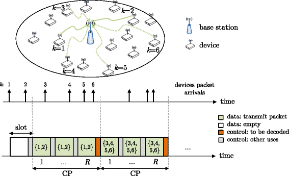
Slotted random access assisted by retransmission diversity and MPR for FF-NDMA with R = 3. The frame is composed of contention periods (CPs), each containing R consecutive time slots. Devices access the shared channel whenever they have a packet to transmit at the CP start. As an example, two and four devices transmit in the first and second CPs, respectively
The single-packet buffer assumption is useful to emulate MTC scenarios where packets are generated every certain period of time (e.g., by sensors) and in which a single-packet buffer is enough to report the latest information.
Stability has been defined in literature for infinite-user as well as for infinite-buffer systems, but not for finite-user single-buffer systems.
We compare FF-NDMA not only with NDMA but also with H-NDMA, since H-NDMA significantly outperforms NDMA at low SNR regimes (i.e., the common operational range for MTC devices that use low order constellations).
H-NDMA matches NDMA operation in Fig. 2 under high SNR regime.
Fig. 2 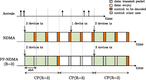
Slotted random access for NDMA and FF-NDMA with R=3. In NDMA, decoding control signaling at every time slot is needed. In FF-NDMA, control signaling has to be decoded only at those CPs in which packets were transmitted
We assume that antenna precoding at the transmitter side entails additional complexity and energy consumption at the base band processing.
If the channel was static and constant among time slots, then the fast-fading channel assumption could be achieved by ensuring that each terminal adds a different random phase for transmission in every time slot.
The waiting time includes the waiting time in the backlog as well as the waiting time for the CP to start.
Recall that, in FF-NDMA, the BS can decode at most \(\tilde {R} {=} RN\) packets at each CP.


References
T Taleb, A Kunz, Machine type communications in 3GPP networks: potential, challenges and solutions. IEEE Commun. Mag. 50(3), 178–184 (2012).
A Al-Fuqaha, et al., Internet of things: a survey on enabling technologies, protocols and applications. IEEE Commun. Surv. Tutor. 17(4), 2347–2376 (2015).
A Bader, et al., First mile challenges for large-scale IoT. IEEE Commun. Mag. 55(3), 138–144 (2017).
H Shariatmadari, et al., Machine-type communications: current status and future perspectives toward 5G systems. IEEE Commun. Mag. 53(9), 10–17 (2015).
A Laya, L Alonso, J Alonso-Zarate, Is the random access channel of LTE and LTE-A suitable for M2M communications? A survey of alternatives. IEEE Tutor. Surv. Commun. Mag. 16(1), 4–16 (2014).
3GPP Long term evolution (LTE). www.3gpp.org/. Accessed Feb 2018.
So J, et al., LoRaCloud: LoRa platform on OpenStack, IEEE NetSoft Conf. and Workshops, (Seoul, 2016).
Revised WI: further LTE physical layer enhancements for MTC. RP-150492, ericsson, RAN 67, Shanghai, China.
TPC de Andrade, et al., The random access procedure in long term evolution networks for the internet of things. IEEE Commun. Mag. 55(3), 124–131 (2017).
R Ratasuk, et al., Narrowband LTE-M system for M2M communication, IEEE Vehicular Technology Conf, (Vancouver, 2014).
Y-P Wang, et al., A primer on 3GPP narrowband internet of things. IEEE Commun. Mag. 55(3), 117–123 (2017).
R Ratasuk, et al., NB-IoT system for M2M communication, IEEE Wireless Commun. and Networking Conf, 1–5 (2016).
3GPP RP-150492, Ericsson, Revised WI: Further LTE Physical Layer Enhancements for MTC. TSG RAN Meeting 67, Shanghai, China, 9-12 Mar. 2015.
S Ghez, S Verdú, SC Schwartz, Stability properties of slotted ALOHA with multipacket reception capability. IEEE Trans. Autom. Control. 33(7), 640–649 (1988).
R Nelson, L Kleinrock, The spatial capacity of a Slotted ALOHA multihop packet radio network with capture. IEEE Trans. Commun. 32(6), 684–694 (1984).
S Ghez, S Verdu, SC Schwartz, Optimal decentralized control in the random access multipacket channel. IEEE Trans. Autom. Control. 34(11), 1153–1163 (1989).
J-L Lu, W Shu, M-Y Wu, A survey on multipacket reception for wireless random access networks. J. Comput. Netw. Commun.2012:, 14 (2012). Article ID 246359. https://doi.org/10.1155/2012/246359.
M Tsatsanis, R Zhang, S Banerjee, Network-assisted diversity for random access wireless networks. IEEE Trans. Sign. Process. 48(3), 702–711 (2000).
R Zhang, M Tsatsanis, Network-assisted diversity multiple access in dispersive channels. IEEE Trans. Commun. 50(4), 623–632 (2002).
N Souto, et al., Iterative multipacket detection for high throughput transmissions in OFDM systems. IEEE Trans. Commun. 58(2), 429–432 (2010).
R Zhang, ND Sidiropoulos, M Tsatsanis, Collision resolution in packet radio networks using rotational invariance techniques. IEEE Trans. Commun. 50(1), 146–155 (2002).
B Ozgul, H Delic, Wireless access with blind collision-multiplicity detection and retransmission diversity for quasi-static channels. IEEE Trans. Commun. 54(5), 858–867 (2006).
R Dinis, et al., Frequency-domain multipacket detection: a high throughput technique for SC-FDE systems. IEEE Trans. Wirel. Commun. 8(7), 3798–3807 (2009).
Pereira M, et al., Optimization of a p-persistent network diversity multiple access protocol for a SC-FDE System. IEEE Trans. Wirel. Commun. 12(12), 5953–5965 (2013).
R Robles, et al., A random access protocol incorporating multi-packet reception, retransmission diversity and successive interference cancellation, 8th Int. Workshop on Multiple Access Commun. (MACOM2015), (Helsinki, 2015).
R Samano-Robles, Network diversity multiple access with imperfect channel state information at the transmitter side. Adv. Wirel. Optim. Commun. (2016).
R Robles, et al., Network diversity multiple access in Rayleigh fading correlated channels with imperfect channel and collision multiplicity estimation, 24th Telecommunications Forum (TELFOR), (Belgrade, 2016).
G Dimic, ND Sidiropoulos, L Tassiulas, Wireless networks with retransmission diversity access mechanisms: stable throughput and delay properties. IEEE Trans. Sign. Process. 51(8), 2019–2030 (2013).
R Samano-Robles, M Ghogho, DC McLernon, Wireless networks with retransmission diversity and carrier-sense multiple access. IEEE Trans. Sign. Process. 57(9), 3722–3726 (2009).
R Samano-Robles, A Gameiro, Stability properties of network diversity multiple access protocols with multiple antenna reception and imperfect collision multiplicity estimation. J. Comput. Netw. Commun. 2013:, 10 (2013). Article ID 984956. http://dx.doi.org/10.1155/2013/984956.
F Ganhao, et al., Performance analysis of an hybrid ARQ adaptation of NDMA schemes. IEEE Trans. Commun. 61(8), 3304–3317 (2013).
M Madueño, J Vidal, Joint physical-MAC layer design of the broadcast protocol in ad-hoc networks. IEEE J. Sel. Areas Commun. 23(1), 65–75 (2005).
M Madueño, J Vidal, PHY-MAC performance of a MIMO network-assisted multiple access scheme, IEEE 6th Workshop on Signal Process. Advances in Wireless Commun, (New York, 2005).
3GPP TR 38.912, Study on New Radio (NR) access technology. Release 14, V14.0.0, Mar. 2017.
3GPP TS 36.213, Evolved Universal Terrestrial Radio Access (E-UTRA); Physical Layer Procedures. v9.2.0, Jun. 2010.
3GPP TR 36.814, Further advancements for E-UTRA physical layer aspects. Release 9, v9.0.0, Mar. 2010.
EG Larsson, P Stoika, Space-time block coding for wireless communications (Cambridge University Press, The Edinburgh Building, 2003).
V Tarokh, H Jafarkhani, RA Calderbank, Space-time block codes from orthogonal designs. IEEE Trans. Inf. Theory. 45(5), 1451–1458 (1999).
D Tse, P Viswanath, Fundamentals of wireless communications (Cambridge University Press, The Edinburgh Building, 2004).
ST Chung, A Goldsmith, Degrees of freedom in adaptive modulation: a unified view. IEEE Trans. Commun. 49(9), 1561–1571 (2001).
JG Proakis, M Salehi, Digital communications, 5th ed. McGraw-Hill (The McGraw-Hill Companies, Inc., New York, 2008).
R Rom, M Sidi, Multiple access protocols: performance and analysis (Springer Verlag, New York, 1990).
L Kleinrock, Theory, Volume 1, Queueing systems. Wiley-Interscience (Wiley, New York, 1975).
JDC Little, A proof for the queuing formula: L= λW. Oper. Res. 9(3), 383–387 (1961).
A Zappone, E Jorswieck, Energy efficiency in wireless networks via fractional programming theory. Found. Trends Communun. Inf. Theory. 11(3-4), 185–701 (2014).
B Dai, W Yu, Sparse beamforming and user-centric clustering for downlink cloud radio access network. IEEE Access Special Section Recent Adv. C-RAN. 2:, 1326–1339 (2014).
Andreev S, et al., Efficient small data access for machine-type communications in LTE, EEE Int. Conf. Commun, 3569–3574 (2013).
P Grover, K Woyach, A Sahai, Towards a communication-theoretic understanding of system-level power consumption. EEE J. Sel. Areas Commun. 29(8), 1744–1755 (2011).
Acknowledgements
This work has been partially funded by the Spanish Ministerio de Economía, Industria y Competitividad and FEDER funds through project TEC2016-77148-C2-1-R (AEI/FEDER, UE): 5G &B RUNNER-UPC, and by the Catalan Government through the grant 2017 SGR 578 - AGAUR.
Author information
Authors and Affiliations
Contributions
SL, AA, and JV put forward the idea. SL, AA, and JG did the mathematical development. SL and JG carried out the experiments. SL wrote the manuscript. JV took part in the discussions and he also guided, reviewed, and checked the writing. All authors contributed to the interpretation of the results and read and approved the final manuscript.
Corresponding author
Ethics declarations
Competing interests
The authors declare that they have no competing interests.
Publisher’s Note
Springer Nature remains neutral with regard to jurisdictional claims in published maps and institutional affiliations.
Rights and permissions
Open Access This article is distributed under the terms of the Creative Commons Attribution 4.0 International License(http://creativecommons.org/licenses/by/4.0/), which permits unrestricted use, distribution, and reproduction in any medium, provided you give appropriate credit to the original author(s) and the source, provide a link to the Creative Commons license, and indicate if changes were made.
About this article

Cite this article
Lagen, S., Agustin, A., Vidal, J. et al. Performance analysis of feedback-free collision resolution NDMA protocol. J Wireless Com Network 2018, 45 (2018). https://doi.org/10.1186/s13638-018-1049-x
Received:
Accepted:
Published:
DOI: https://doi.org/10.1186/s13638-018-1049-x