- Research
- Open access
- Published:
Performance analysis of cognitive underlay two-way relay networks with interference and imperfect channel state information
EURASIP Journal on Wireless Communications and Networking volume 2018, Article number: 53 (2018)
Abstract
In this paper, we evaluate two-way relay communication systems in cognitive radio environments. The proposed model includes two subsystems: a primary system and a secondary system. The primary system consists of a primary transmitter and a primary receiver while the secondary includes two terminals exchanging their data via an intermediate relay node. Each network node is equipped with a single antenna and operates under a half-duplex mode. The channel state information (CSI) interference from the secondary node to the primary receiver is assumed imperfect. Using analytical methods, this paper derives the interference probability from the secondary system to the primary receiver and an optimal back-off control power coefficient for the secondary transmitter. To evaluate the secondary system quality, an explicit expression for the system outage probability (OP) and its closed form in the high signal-to-noise region (SNR) is presented. Theoretical results are verified using Monte-Carlo simulation.
1 Introduction
Rapid development of wireless networks coupling with a large number of users and requirements for high-speed wireless services leads to radio frequency spectrum scarcity. Many researchers have enhanced the spectrum efficiency using various methods such as multiplexing and modulation, which are also useful for overcoming fading severity. However, it appears that the current available approaches only enhance a portion of the vast available spectral efficiency rather than potentially being long-term approaches for the next wireless generation systems. Recently, cognitive radio has been proposed as a promising technique to address spectral efficiency problem. It is clear that cognitive radio techniques widen radio spectrum access, where unlicensed users are allowed to operate in the same frequency band allocated to licensed users. Therefore, in the current cognitive radio medium, there are two main systems: the primary system and the secondary system. To detect spectral opportunities, various spectrum sensing algorithms are presented, where energy detection-based spectrum sensing is an effective and simple detection technique [1–3].
Cognitive radio techniques have not only attracted researchers from academia worldwide but also gaining attention from the industry and governments. As such, these techniques have increasingly become one of the main research areas, and many findings have been published on the topic including the use of (i) multiple input, multiple output (MIMO) technologies [4, 5], (ii) relay selection [6, 7], (iii) multi-hop relaying [8, 9], (iv) physical layer security [10], (v) energy harvesting technologies [11, 12], and (vi) a new system model to analyze system quality [13–15].
In conventional wireless systems, the two-way transmission technique not only enhances spectral efficiency but also allows extended coverage [16]. Therefore, this technique has received considerable researchers’ attention in recent years. For this technique, there are two basic signal processing methods being employed at the intermediate relay node: AF (amplify and forward) and DF (decode and forward). Most existing studies apply these methods in two-phase two-way or three-phase two-way relay transmission protocols [17]. Furthermore, some studies have evaluated two-way systems in Nakagami-m fading [18] and also in other fading channels [19].
Combining the two-way relay transmission technique with cognitive radio, one significantly increases system spectral efficiency. In [20], Duy et al. analyzed the quality of two-way relay transmission secondary systems in which their model includes three-phase DF relay intermediate nodes. Furthermore, they obtained exact expressions for the system outage probability in Rayleigh fading. For two-way DF relaying systems in cognitive radio environments, Afana et al. derived exact expressions for the system outage probability and bit error rate in a two-way system, consisting of several relay nodes, primary transmitters and primary receivers [21–23] which are important findings for further developments on cognitive relay radio techniques. However, Afana’s analytical results are only correct for system models with a large number of relay nodes and a limited number of primary receivers. To overcome this bottleneck, the authors in [24] offered exact expressions for the system outage probability where the numbers of relay nodes and primary receivers are allowed to be arbitrary in Nakagami-m fading. Considering AF two-way relay transmission systems employing massive MIMO, the authors in [25] solved for the optimal beamforming power allocation and optimal coefficients. One of the most important contributions to the literature is presented by Zhang et al. [26], in which the authors evaluated system quality and gave exact expressions for system outage probability when considering interference effects from the primary transmitter to the secondary network nodes. It is noted that the common feature of most current contributions is only to consider two-way systems for perfect channel state information (CSI).
It is also clear that because of continuous random variation of fading channels and channel estimation errors, perfect CSI is practically difficult to acquire. For cognitive radio systems, if the transmitters in the secondary system do not have perfect CSI, these equipments don’t effectively and efficiently control their required transmit power, increasing interference to the primary receivers and subsequently affect the primary system operation. Therefore, cognitive radio system quality evaluation under imperfect CSI conditions is necessary as the findings can be used to verify theoretical prediction against practical data. In [27], the authors considered a system model that has two secondary terminals and a number of intermediate relay nodes in cognitive radio environments. Their proposed system is mathematically modeled and solved to obtain optimal beamforming for two cases: perfect CSI and imperfect CSI. However, these authors did not consider interference effects from the primary transmitters to the secondary system. Considering mutual interference between the primary network and the secondary network, the authors in [28] focused on analyzing the system under imperfect CSI condition. In addition, relay systems’ quality is analyzed in cognitive radio environments for imperfect CSI such as [29] evaluated the multi-stage secondary system quality, while [30] studied a cooperative transmission secondary system in Nakagami-m fading.
To the best of our knowledge, the findings on evaluating two-way relay transmission system’ quality in cognitive radio environments considering interference from the primary transmitters to the secondary system with imperfect CSI from the secondary network nodes to the primary receivers are not yet available. The contribution of the paper thus are:
-
Deriving the interference probability from the secondary system to primary receivers for imperfect CSI;
-
Obtaining power back-off coefficients for secondary network nodes’ transmitters to ensure satisfactory interference probability from primary receivers is achieved;
-
Deriving an exact expression for the secondary system outage probability;
-
Offering an asymptotic outage probability (OP) formula for the secondary system in the high SNR region and determining the system diversity order.
The paper is organized as follows: Section 2 outlines the proposed system model. The outage probability for the secondary system is studied in Section 3 while Section 4 presents simulation results. Section 5 concludes the main findings of this paper and gives possible future work.
2 System model
Figure 1 shows the system model which includes network nodes of the primary network and the secondary network. The primary network consists of a primary transmitter PU-Tx and a primary receiver PU-Rx while the secondary network consists of two terminals A and B exchanging data via the intermediate relay node R. It is assumed that each network node is equipped with a singe antenna and operates in the half-duplex mode.

Cognitive underlay two-way relaying networks with interference and imperfect channel state information
The channel coefficient from node X to node Y is denoted as hXY, where X,Y∈{A,B,R,P}. The interference channel from the secondary nodes to the primary receiver (PU-Rx) is hXP, and the interference channel from the primary transmitter (PU-Tx) to secondary nodes is hPX with X∈{A,B,R}. It is assumed that all channels experience flat independent Rayleigh fading. Therefore, the channel gain from node X to node Y, |hXY|2, is an exponential-distributed random variable having the cumulative distribution function (CDF) and probability density function (PDF) given as
where \(\lambda _{\text {XY}}= \mathbb {E}\{|h_{\text {XY}}|^{2}\}\) with \(\mathbb {E}\{.\}\) being expectation operator.
The two-way relay transmission process between node A and node B occurs in three phases, and relay node R processes its received signals using DF relaying. In the first phase, node A transmits its signals to node R. Then, node B transmits its signals to node R in the second phase. Finally, the relay decodes and encodes its received signals from node A and node B before broadcasting these signals to the two terminals in the third phase.
Since the secondary system operates at the primary system frequency band, the transmit power of the secondary network nodes has to be adjusted to ensure that interference \({\widetilde I_{\mathrm {p}}}\) to the receiver PU-Rx is kept under a threshold. Thus, if the secondary nodes fully possess the interference CSI at the primary receiver, the best transmit power of the secondary nodes can be defined as
However, in practice, perfect CSI of the interference links from secondary transmitters to the primary receiver is not available at the corresponding secondary transmitters because of channel estimation errors or time-varying impairments, is possibly caused by the combination of channel estimation error, mobility, feedback delay, and limited feedback. Therefore, interference channel coefficients from the secondary node X to the primary receiver Y are often estimated as \({\hat h_{{\text {XP}}}}\), which are different from the exact channel coefficients, mathematically described as [31]
where ξXP is a complex symmetric zero-mean Gaussian random variable with the variance λXP, and ρ is a correlation coefficient between the real channel and the estimated channel. This correlation coefficient can be determined using a pilot symbol modulated parameter (PSAM) [32]. For Rayleigh fading channels, the joint PDF of \({\left | {{{\hat h}_{{\text {XP}}}}} \right |^{2}}\) and |hXP|2 is defined as [31]
where \({I_{0}}\left (x \right) = \frac {1}{\pi }\int _{0}^{\pi } e^{x\cos {\theta }} d\theta \) is the zeroth-order modified Bessel function of the first kind.
From (5), we obtain the PDF of \(|{\hat h}_{\text {XP}}|^{2}\) as [33]
As a result, the best transmit power of the secondary network nodes for imperfect CSI can be defined as
In the first phase, the received signal at node R from node A can be written as
where xX is the transmit symbol of node X with \({\mathbb {E}}\left \{ {|x_{\mathrm {X}}|^{2}} \right \} = 1\); \({n_{\mathrm {R}}^{k}} \sim {\mathcal {N}}\left ({0,{N_{0}}} \right)\) is additive white Gaussian noise (AWGN) at phase k with zero mean and variance of N0. In addition, xP and PPU−Tx are the transmit symbol and the transmit power of the primary transmitter PU-Tx, respectively, with \({\mathbb {E}}\left \{ {|x_{\mathrm {P}}|^{2}} \right \} = 1\). Similarly, we can write the received signal at node R from node B in the second phase as
Therefore, the signal power to noise and interference ratio of the received signal at R in the first and second phases can be given, respectively, by
and
In the third phase, relay node R adjusts its transmit power to keep interference at the primary receiver input under a threshold \({\widetilde I_{\mathrm {p}}}\). The received signal at terminal X with X∈{A,B} in the third phase is given as
where \({n_{\mathrm {X}}} \sim {\mathcal {N}}\left ({0,{N_{0}}} \right)\) is AWGN at the receiver input of terminal node X, and xR is the transmit symbol of relay node R with \({\mathbb {E}}\left \{ |{x_{\mathrm {R}}}|^{2} \right \} = 1\).
Thus, the simultaneous signal power to interference ratio at the two terminals A and B can be given by
and
3 Performance analysis
In this section, we study the performance of primary and secondary networks. For the primary networks, we consider the interference probability. For the secondary networks, we derive the system outage probability and its asymptotic expression at high SNR regime.
3.1 Primary networks: interference probability analysis
The interference probability is defined as the probability that the interference from secondary transmitters received at the primary transmitters is greater than the interference threshold, Ip. Considering three communications phases for the secondary networks, we may write the primary interference probability using the theorem of total probability as follows:
Using the result in [29], we straightforwardly arrive at
where \(\Pr \left ({\frac {{{{\left | {{h_{{\text {XP}}}}} \right |}^{2}}}}{{{{| {{{\hat h}_{{\text {XP}}}}} |}^{2}}}} > 1} \right) = \frac {1}{2} \) is for Rayleigh fading channels.
To reduce P I , we adopt the back-off technique, i.e., reducing the secondary transmit power to obtain acceptable interference. Denoting δX with 0≤δX≤1 as the back-off power control coefficient of node X, the transmit power of node X can be rewritten as
Applying Lemma 1 in [29], after tedious manipulations, we finally obtain the closed-form expression for the interference probability as
where \({\varphi _{\mathrm {X}}} = \frac {{{\delta _{\mathrm {X}}} - 1}}{{\sqrt {{{\left ({{\delta _{\mathrm {X}}} + 1} \right)}^{2}} - 4{\rho ^{2}}{\delta _{\mathrm {X}}}} }}\) with X∈{A, B, R}.
Applying the arithmetic-geometric inequality ([34], Eq. (11.116)) for three positive numbers \(\frac {{1 - {\varphi _{\mathrm {A}}}}}{2}\), \(\frac {{1 - {\varphi _{\mathrm {B}}}}}{2}\), and \(\frac {{1 - {\varphi _{\mathrm {R}}}}}{2}\) in (18), we have
From (19), it appears that the interference probability can achieve its minimum if and only if δA=δB=δR=δ, where \(\varphi = \frac {{\delta - 1}}{{\sqrt {{{\left ({\delta + 1} \right)}^{2}} - 4{\rho ^{2}}\delta } }}\).
The minimum of P I may be given as
for an equi-correlation coefficient ρ in all interference channels.
Although the back-off power control technique is useful in obtaining satisfactory P I , it also degrades the secondary network performance. Thus, it is necessary to calculate the back-off power control peak coefficient for a given P I . Using the analysis method as in [29], we can find the back-off power control peak coefficient as follows:
where \(\kappa = 2\sqrt [3]{{1 - {P_{I}}}} - 1\).
3.2 Secondary two-way relaying networks
In this section, the performance of cognitive underlay two-way relaying networks over Rayleigh fading channels is studied starting with the instantaneous SNRs at the receiving nodes using the back-off coefficient. In particular, we obtain the SNR at R in the first and second phase, respectively, as follows:
and
For the third phase, we have the SNRs at A and B, respectively, as
and
For two-way DF relaying, the secondary system outage probability can be written as
where γe is defined as
and γth is the given SNR threshold.
Assuming that γ′AR, γ′BR, and γe are independent of each other, we may write
where F Z (z) is the CDF of Z.
In order to derive the exact expression of the system outage probability, we consider the following Lemma.
Lemma 1
Let X and Y are exponentially distributed random variables with means λX and λY, respectively, and Z is a random variable defined as \(Z = \frac {X}{{\text {PY} + 1}}\), where \({\mathrm {P}} > 0,\,\,{\mathrm {P}} \in {\mathbb {R}}\). The CDF of Z can be given as
Proof
We have
Applying ([34], eq. (3.31011)), we obtain the CDF of Z as (29). □
Then, the exact closed-form expression for the system OP is stated in Theorem 1.
Theorem 1
For a given ρ, the closed-form expression for the system outage probability over Rayleigh fading channels is
where Ei(·) is the exponential integral [27, Eq. (8.211)], \({m_{1}} = \frac {{{\delta _{\mathrm {A}}}{I_{\mathrm {p}}}{\lambda _{{\text {AR}}}}}}{{{\gamma _{{\text {th}}}}P{\lambda _{{\text {PR}}}}}}\), \({m_{2}} = \frac {{{\delta _{\mathrm {B}}}{I_{\mathrm {p}}}{\lambda _{{\text {BR}}}}}}{{{\gamma _{{\text {th}}}}P{\lambda _{{\text {PR}}}}}}\), \({k_{1}} = \frac {{{\gamma _{{\text {th}}}}}}{{{\delta _{\mathrm {A}}}{I_{\mathrm {p}}}{\lambda _{{\text {AR}}}}}} + \frac {1}{{{\lambda _{{\text {AP}}}}}}\), \({k_{2}} = \frac {{{\gamma _{{\text {th}}}}}}{{{\delta _{\mathrm {B}}}{I_{\mathrm {p}}}{\lambda _{{\text {BR}}}}}} + \frac {1}{{{\lambda _{{\text {BP}}}}}}\), \({x_{1}} = \frac {{{\delta _{\mathrm {R}}}{I_{\mathrm {p}}}{\lambda _{{\text {RA}}}}}}{{{\gamma _{{\text {th}}}}P{\lambda _{{\text {PA}}}}}}\), \({x_{2}} = \frac {{{\delta _{\mathrm {R}}}{I_{\mathrm {p}}}{\lambda _{{\text {RB}}}}}}{{{\gamma _{{\text {th}}}}P{\lambda _{{\text {PB}}}}}}\), \(\phi = \frac {{{\gamma _{{\text {th}}}}}}{{{\delta _{\mathrm {R}}}{I_{\mathrm {p}}}{\lambda _{{\text {RA}}}}}} + \frac {{{\gamma _{{\text {th}}}}}}{{{\delta _{\mathrm {R}}}{I_{\mathrm {p}}}{\lambda _{{\text {RB}}}}}}\), and \(\psi = \frac {{\delta _{\mathrm {R}}^{2}I_{\mathrm {p}}^{2}{\lambda _{{\text {RA}}}}{\lambda _{{\text {RB}}}}}}{{\gamma _{{\text {th}}}^{2}{P^{2}}{\lambda _{{\text {PA}}}}{\lambda _{{\text {PB}}}}}}\).
Proof
From (26), we can see that the explicit expression for the system outage probability in (28) can be defined after determining the CDF of \({\gamma ^{\prime }_{{\text {AR}}}}\), \({\gamma ^{\prime }_{{\text {BR}}}}\), and γe.
We first consider the CDF of \({\gamma ^{\prime }_{{\text {AR}}}}\). Using the conditional probability, we can write the CDF of \({\gamma ^{\prime }_{{\text {AR}}}}\) as
where \(F_{{\left. \gamma ^{\prime }_{\text {AR}} \right |} |h_{\text {AP}}|^{2}}(\gamma _{\text {th}}|x)\) is the CDF of \({\gamma ^{\prime }_{{\text {AR}}}}\) conditioned on |hAP|2 and \(f_{|h_{\text {AP}}|^{2}}(x)\) is the PDF of |hAP|2.
Recalling (10) and (22), we can write
where \({I_{\mathrm {P}}} = {\tilde I_{\mathrm {p}}}/{N_{0}}\) and P=PPU−Tx/N0.
Applying the result of Lemma 1, where X,Y, and z correspond |hAR|2, |hPR|2, and \( \frac {{x{\gamma _{{\text {th}}}}}}{{{\delta _{\mathrm {A}}}{I_{\mathrm {P}}}}}\), respectively, we have
Substituting (34) and (2) into (35), we have
Using ([34], Eq. (3.352.4)), we obtain
where \({m_{1}} = \frac {{{\delta _{\mathrm {A}}}{I_{\mathrm {p}}}{\lambda _{{\text {AR}}}}}}{{{\gamma _{{\text {th}}}}P{\lambda _{{\text {PR}}}}}}\) and \({k_{1}} = \frac {{{\gamma _{{\text {th}}}}}}{{{\delta _{\mathrm {A}}}{I_{\mathrm {p}}}{\lambda _{{\text {AR}}}}}} + \frac {1}{{{\lambda _{{\text {AP}}}}}}\).
Here, we note that \({\gamma ^{\prime }_{{\text {AR}}}}\) and \({\gamma ^{\prime }_{{\text {BR}}}}\) take the same form. Similarly, the CDF of \({\gamma ^{\prime }_{{\text {BR}}}}\) can be given by
where \({m_{2}} = \frac {{{\delta _{\mathrm {B}}}{I_{\mathrm {p}}}{\lambda _{{\text {BR}}}}}}{{{\gamma _{{\text {th}}}}P{\lambda _{{\text {PR}}}}}}\) and \({k_{2}} = \frac {{{\gamma _{{\text {th}}}}}}{{{\delta _{\mathrm {B}}}{I_{\mathrm {p}}}{\lambda _{{\text {BR}}}}}} + \frac {1}{{{\lambda _{{\text {BP}}}}}}\).
We are now in a position to derive the CDF of \({F_{{\gamma _{e}}}}\left ({{\gamma _{{\text {th}}}}} \right)\). Making use the fact that γRA and γRB are correlated due to the common random variable \(\left | {{{\hat h}_{{\text {RP}}}}} \right |^{2}\), we can write the CDF of \({F_{{\gamma _{e}}}}\left ({{\gamma _{{\text {th}}}}} \right)\) as
where \({F_{{\gamma _{\mathrm {e}}}\left | {\left | {{{\hat h}_{{\text {RP}}}}} \right |^{2}} \right.}}\left ({{\gamma _{{\text {th}}}}\left | x \right.} \right)\) denotes the CDF of γe conditioned on \(\left | {{{\hat h}_{{\text {RP}}}}} \right |^{2}\) given by
Applying Lemma 1 for the second term in (39), where X,Y, and z correspond |hRA|2, |hPA|2, and \(\frac {{x{\gamma _{{\text {th}}}}}}{{{\delta _{\mathrm {R}}}{I_{\mathrm {P}}}}}\), respectively, we have
where \({x_{1}} = \frac {{{\delta _{\mathrm {R}}}{I_{\mathrm {p}}}{\lambda _{{\text {RA}}}}}}{{{\gamma _{{\text {th}}}}P{\lambda _{{\text {PA}}}}}}\). Similarly, we have
where \({x_{2}} = \frac {{{\delta _{\mathrm {R}}}{I_{\mathrm {p}}}{\lambda _{{\text {RB}}}}}}{{{\gamma _{{\text {th}}}}P{\lambda _{{\text {PB}}}}}}\).
Substituting (40), (41), and (39) into (38), we obtain
where \(\phi = \frac {{{\gamma _{{\text {th}}}}}}{{{\delta _{\mathrm {R}}}{I_{\mathrm {p}}}{\lambda _{{\text {RA}}}}}} + \frac {{{\gamma _{{\text {th}}}}}}{{{\delta _{\mathrm {R}}}{I_{\mathrm {p}}}{\lambda _{{\text {RB}}}}}}\) and \(\psi = \frac {{\delta _{\mathrm {R}}^{2}I_{\mathrm {p}}^{2}{\lambda _{{\text {RA}}}}{\lambda _{{\text {RB}}}}}}{{\gamma _{{\text {th}}}^{2}{P^{2}}{\lambda _{{\text {PA}}}}{\lambda _{{\text {PB}}}}}}\). Applying ([34], Eq. (3.352.4)), one has
Substituting (36), (37), and (43) into (28), we obtain an exact expression for the secondary system outage probability, when the interference CSI to the primary receiver is imperfect as in (31). □
3.2.1 Asymptotic system outage probability at high SNR regime
By using \(1 - {e^{- x}}\mathop \approx \limits ^{x \to 0} x\), the approximate CDF expression for \({\gamma ^{\prime }_{{\text {AR}}}}\), \({\gamma ^{\prime }_{{\text {BR}}}}\), and γe over the high SNR region can be calculated, so that the corresponding asymptotic system outage probability can be found.
Theorem 2
Over Rayleigh fading channels, the asymptotic system outage probability at high SNR regime is of the form as (44).
Proof
We start the proof from the definition of \(\phantom {\dot {i}\!}{F_{{{\gamma ^{\prime }}_{{\text {AR}}}}}}\left ({{\gamma _{{\text {th}}}}} \right)\) as
Based on the exponential approximate property, we are able to find the approximate CDF for \({\gamma ^{\prime }_{{\text {AR}}}}\) as
Using ([34], Eq. (3.351.3)) for the inner integral of (46), we have
Utilizing similar analytical steps, we find the approximate CDF expression for \({\gamma ^{\prime }_{{\text {BR}}}}\) as
For the approximate CDF expression for γe, from (39), we have
We first calculate I1 as follows:
Similarly, we have I2 given by
Substituting I1 in (50) and I2 in (51) into (49), we can define the approximate CDF expression for γ e as
With the help of ([34], Eq. (3.351.3)), we derive the closed-form CDF expression for γe in the high SNR region as
Substituting (47), (48), and (53) into (28), we obtain the approximate expression for the system outage probability in the high SNR region as in (44).
From (44), for Ip→+∞, we have
where
□
Therefore, it can be seen that over the high SNR region, the system outage probability is proportional to \(\frac {1}{{{I_{\mathrm {p}}}}}\). It can be shown that over the high SNR region, the system diversity is one.
4 Numerical results and discussion
In this section, the analytical results are verified using Monte-Carlo simulation. It is assumed that the system network nodes lie on a plane coordinate system Oxy, and the distance between node A and node B is normalized to 1. Therefore, for simulation purposes, the two secondary terminals are placed at A[0; 0], B[1; 0], PU-Tx[0; 1], and PU-Rx[1; 1], respectively, and the relay node is located at R[0,5; 0]. dMN is the physical distance between two network nodes M and N, where M,N∈{A, B, R, PU−Rx, PU−Tx}. For free-space path loss transmission, we have λMN=dMN−η, where η is a path loss exponent, 2≤η≤6. For simulation purposes, the following are also used: η=3, γth=1.25, δA=δB=δR=δmax, and P = 20 dB.
Figure 2 shows the secondary system interference probability to the primary receiver (P I ) as a function of ρ for three cases: δ=0.35, δ=0.5, and δ=0.75. It can be seen that our theoretical prediction and the simulation results are consistent, verifying our analyses. Furthermore, P I is an inverse function of ρ, and there appears a singularity for ρ→1Footnote 1.
In Fig. 3, the secondary system outage probability for (i) when the correlation coefficient ρ is varied and (ii) P I =0.05, P = 20 [dB] is presented, from which our analytical results are consistent with the simulation results, verifying our derivation approach. Furthermore, the severity of the correlation coefficient ρ to the secondary system quality is revealed when the secondary transmitters adjust their power following the back-off power δmax.

Effect of the correlation coefficient on the secondary system outage performance
Figure 4 presents the secondary system outage probability when the interference channel to the primary receiver is imperfect with a correlation coefficient ρ=0.98 for P=20 dB. The system is also simulated for P I =0.2,P I =0.1, and P I =0.05. It can be seen from Fig. 4 that reducing the interference probability degrades the secondary system quality. This is because the decrease in the interference probability P I leads to the decrease of the back-off factor. Therefore, the secondary network nodes’ transmit power decreases, hence increasing the secondary system outage probability.

Effect of P I on the secondary system outage performance
5 Conclusion
This paper studies the DF two-way relay transmission system in cognitive radio environments. Furthermore, our proposed model considers the primary transmitter interference to the secondary system and evaluates the system quality when the interference CSI from the secondary transmitters to the primary receiver is imperfect. This paper has derived the interference probability to the primary receiver, the maximum back-off power factor which is used to keep interference under a threshold level. For the secondary system, an exact expression for the system outage probability and its asymptotic expression for the high SNR region have been obtained. These new findings have been verified using the Monte-Carlo simulation results. Further studies on two-way relay systems with imperfect CSI at the primary transmitters will be reported in a separate publication.
Notes
ρ can be assumed less than 1 to avoid the singularity.
Fig. 2 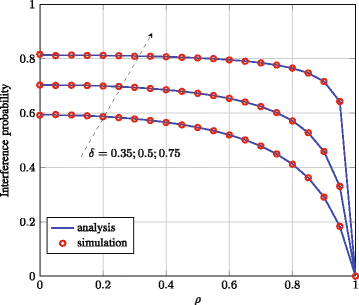
Effect of the correlation coefficient on the interference probability P I to the primary receiver

References
MR A Singh, RK Bhatnagar, Mallik, Cooperative spectrum sensing in multiple antenna based cognitive radio network using an improved energy detector. IEEE Commun. Lett. 16(1), 64 (2012).
MR A Singh, RK Bhatnagar, Mallik, Performance of an improved energy detector in multihop cognitive radio networks. IEEE Trans. Veh. Technol. 65(2), 732 (2016).
D Goel, VS Krishna, M Bhatnagar, Selection relaying in decode-and-forward multi-hop cognitive radio systems using energy detection. IET Commun. 10(7), 753 (2016).
G Scutari, DP Palomar, S Barbarossa, Cognitive MIMO radio. IEEE Signal Process. Mag. 25(6), 46 (2008).
A Alsharoa, H Ghazzai, MS Alouini, Optimal transmit power allocation for MIMO two-way cognitive relay networks with multiple relays using AF strategy. IEEE Wireless Commun. Lett.3(1), 30 (2014).
K Ho-Van, Exact outage analysis of modified partial relay selection in cooperative cognitive networks under channel estimation errors. IET Commun. 10(2), 219 (2016).
VNQ Bao, TQ Duong, Exact outage probability of cognitive underlay DF relay networks with best relay selection. IEICE Trans. Commun.E95.B(6), 2169 (2012).
HK Boddapati, MR Bhatnagar, S Prakriya, in 2016 IEEE Globecom Workshops (GC Wkshps). Ad-hoc relay selection protocols for multi-hop underlay cognitive radio networks. (Washington, 2016), pp. 1–6.
HK Boddapati, S Prakriya, MR Bhatnagar, in 2017 IEEE Int. Conf. Commun. Workshops (ICC Workshops). Throughput analysis of cooperative multi-hop underlay CRNs with incremental relaying. (Paris, 2017), pp. 379–385.
AG Fragkiadakis, EZ Tragos, IG Askoxylakis, A survey on security threats and detection techniques in cognitive radio networks. IEEE Commun. Surveys & Tutorials. 15(1), 428 (2013).
Y Zhang, W Han, D Li, P Zhang, S Cui, Power versus spectrum 2-D sensing in energy harvesting cognitive radio networks. IEEE Trans. Signal Process. 63(23), 6200 (2015).
DK Nguyen, M Matthaiou, TQ Duong, H Ochi, in Proc. 2015 IEEE Int. Conf. Commun. Workshop (ICCW). RF energy harvesting two-way cognitive DF relaying with transceiver impairments. (London, 2015), pp. 1970–1975.
Z Xing, Z Yan, Y Zhi, X Jia, W Wenbo, Performance analysis of cognitive relay networks over Nakagami-m fading channels. IEEE J. Sel. Areas Commun. 33(5), 865 (2015).
B Zhong, Z Zhang, Opportunistic two-way full-duplex relay selection in underlay cognitive networks. IEEE Systems J.PP(99), 1 (2016).
PS Bithas, AA Rontogiannis, K Berberidis, in Proc. 2014 Int. Conf. Wireless and Mobile Comput. Netw. Commun. (WiMob). SINR analysis of cognitive underlay systems with multiple primary transceivers in Nakagami-m fading (Larnaca, 2014), pp. 500–505.
R Boris, W Armin, Spectral efficient protocols for half-duplex fading relay channels. IEEE J. Sel. Areas Commun. 25(2), 379 (2007).
L Song, Relay selection for two-way relaying with amplify-and-forward protocols. IEEE Trans. Veh. Technol. 60(4), 1954 (2011).
Y Jing, F Pingzhi, TQ Duong, L Xianfu, Exact performance of two-way AF relaying in Nakagami-m fading environment. IEEE Trans. Wireless Commun.10(3), 980 (2011).
Z Chensi, G Jianhua, L Jing, R Yun, M Guizani, A unified approach for calculating the outage performance of two-way AF relaying over fading channels. IEEE Trans. Veh. Technol.64(3), 1218 (2015).
TT Duy, HY Kong, Exact outage probability of cognitive two-way relaying scheme with opportunistic relay selection under interference constraint. IET Commun. 6(16), 2750 (2012).
A Afana, A Ghrayeb, V Asghari, S Affes, in Proc. IEEE 14th Workshop Signal Process. Adv. Wireless Commun. (SPAWC). On the performance of spectrum sharing two-way relay networks with distributed beamforming. (2013), pp. 365–369.
A Afana, A Ghrayeb, V Asghari, S Affes, Distributed beamforming for spectrum-sharing systems with AF cooperative two-way relaying. IEEE Trans. Commun. 62(9), 3180 (2014).
A Afana, A Ghrayeb, VR Asghari, S Affes, Distributed beamforming for two-way DF relay cognitive networks under primary-secondary mutual interference. IEEE Trans. Veh. Technol. 64(9), 3918 (2015).
HV Toan, VNQ Bao, in Proc. 2016 International Conference on Advanced Technologies for Communications (ATC). Opportunistic relaying for cognitive two-way network with multiple primary receivers over Nakagami-m fading. (Hanoi, 2016), pp. 141–146.
Y Cao, C Tellambura, Cognitive beamforming in underlay two-way relay networks with multi-antenna terminals. IEEE Trans Cogni. Commun. Netw. 1(3), 294 (2015).
X Zhang, Z Zhang, J Xing, R Yu, P Zhang, W Wang, Exact outage analysis in cognitive two-way relay networks with opportunistic relay selection under primary user’s interference. IEEE Trans. Veh. Technol. 64(6), 2502 (2015).
P Ubaidulla, S Aissa, in Proc. IEEE 22nd Int. Symp. Personal Indoor and Mobile Radio Commun. (PIMRC). Distributed cognitive two-way relay beamformer designs under perfect and imperfect CSI (Toronto, 2011), pp. 487–492.
SH Safavi, M Ardebilipour, S Salari, Relay beamforming in cognitive two-way networks with imperfect channel state information. IEEE Wireless Commun. Lett. 1(4), 344 (2012).
VNQ Bao, TQ Duong, C Tellambura, On the performance of cognitive underlay multihop networks with imperfect channel state information. IEEE Trans. Commun. 61(12), 4864 (2013).
K Ho-Van, PC Sofotasios, S Freear, Underlay cooperative cognitive networks with imperfect Nakagami-m fading channel information and strict transmit power constraint: interference statistics and outage probability analysis. J. Commun. Netw. 16(1), 10 (2014).
HA Suraweera, PJ Smith, M Shafi, Capacity limits and performance analysis of cognitive radio with imperfect channel knowledge. IEEE Trans. Veh. Technol.59(4), 1811 (2010).
X Tang, MS Alouini, AJ Goldsmith, Effect of channel estimation error on M-QAM BER performance in Rayleigh fading. IEEE Trans. Commun. 47(12), 1856 (1999).
M Schwartz, WR Bennett, S Stein, Communication systems and techniques (Wiley-IEEE Press, New York, 1995).
IS Gradshteyn, IM Ryzhik, A Jeffrey, D Zwillinger, Table of integrals, series and products, 7th edn. (Elsevier Amsterdam, Boston, 2007).
Acknowledgements
The authors would like to thank the reviewers for their thorough reviews and helpful suggestions.
Funding
This research work was funded by Vietnam National Foundation for Science and Technology Development (NAFOSTED) under Grant No. 102.04-2014.32.
Availability of data and materials
Not applicable.
Author information
Authors and Affiliations
Contributions
HVT and VNQB proposed the system model, derived the system performance, and performed the simulation and manuscript writing. KNL contributed in the manuscript preparation and manuscript revision. All authors read and approved the final manuscript.
Corresponding author
Ethics declarations
Competing interests
The authors declare that they have no competing interests.
Publisher’s Note
Springer Nature remains neutral with regard to jurisdictional claims in published maps and institutional affiliations.
Additional information
Authors’ information
Not applicable.
Rights and permissions
Open Access This article is distributed under the terms of the Creative Commons Attribution 4.0 International License (http://creativecommons.org/licenses/by/4.0/), which permits unrestricted use, distribution, and reproduction in any medium, provided you give appropriate credit to the original author(s) and the source, provide a link to the Creative Commons license, and indicate if changes were made.
About this article

Cite this article
Toan, H., Bao, V. & Le, K. Performance analysis of cognitive underlay two-way relay networks with interference and imperfect channel state information. J Wireless Com Network 2018, 53 (2018). https://doi.org/10.1186/s13638-018-1063-z
Received:
Accepted:
Published:
DOI: https://doi.org/10.1186/s13638-018-1063-z