Robust full-dimension MIMO transmission based on limited feedback angular-domain CSIT

Stefan Schwarz

doi:10.1186/s13638-018-1070-0

Research
Open Access
Published: 14 March 2018

Robust full-dimension MIMO transmission based on limited feedback angular-domain CSIT

Stefan Schwarz ORCID: orcid.org/0000-0002-4065-2906¹

EURASIP Journal on Wireless Communications and Networking volume 2018, Article number: 58 (2018) Cite this article

1432 Accesses
2 Citations
Metrics details

Abstract

In this paper, we propose robust multi-user beamforming and precoding techniques for full-dimension MIMO transmission based on limited feedback. We propose to employ an over-complete basis decomposition in the angular domain to approximate the channel matrices as sums of few dominant specular components, facilitating efficient channel state information (CSI) quantization at the users. The selected expansion vectors of such a sparse approximation, parametrized by azimuth and elevation angles, are relatively robust with respect to channel estimation errors as well as channel variations over time. Based on this CSI feedback, we propose incoherent beamforming/precoding methods that make use only of the azimuth and elevation angles as well as the norm of the expansion coefficients and do not rely on coherent multipath interference to eliminate inter-user interference. Our optimization aims at maximizing the signal power or the achievable rate of a user, while limiting the amount of interference leakage caused to other users. To further improve robustness, we account for uncertainty in the angular channel decomposition in the proposed precoder optimization.

Introduction

Full-dimension multiple-input multiple-output (FD-MIMO) transmission refers to wireless transmission systems that support two-dimensional antenna arrays with a large number of antenna elements. This enables high-resolution beamforming in both, the elevation and the azimuth domain, in order to achieve space-division multiple access gains through spatial separation of users, as well as to enhance the energy efficiency of wireless data transmission by concentrating the radiated energy towards intended users [1–3]. The great potential of FD-MIMO systems has been recognized by standardization bodies, such as the third generation partnership project (3GPP); correspondingly, development and standardization efforts are ongoing within long-term evolution (LTE) Release 14 and 5G new radio (NR) to further enhance the initial realization of FD-MIMO in Release 13. Currently, most implementation proposals of FD-MIMO transceivers are based on hybrid architectures, where part of the signal processing is performed in base band and part in the analog radio frequency (RF) domain in order to limit the number of required RF chains. This approach is especially important in the millimeter wave band, where hardware complexity is a limiting factor [4–8]. When designing hybrid precoding systems, several challenges need to be addressed [9–11]: the design freedom of RF precoders is commonly restricted by hardware limitations, such as discrete angular resolution and constant modulus of the phase-shifting elements, as well as partial connectivity of the phase-shift network to limit insertion loss. An alternative to hybrid architectures, which potentially provides even higher spectral and energy efficiency in certain operating regimes, is to employ cheap low (even single bit) resolution analog to digital (AD)/digital to analog (DA) converters in FD-MIMO transceivers. At the receive-side of most existing MIMO transceivers, high-resolution AD converters are employed to minimize the signal distortions introduced by the receiver. Such high-resolution AD converters are, however, among the most power hungry devices of the receiver chain. This motivates the use of low-resolution energy efficient AD converters in FD-MIMO systems to achieve energy-efficient operation [12–15]. At the transmit side, on the other hand, power expenditure is dominated by power amplifiers, which are usually required to operate within the high linearity regime to avoid signal distortion. Employing low-resolution DA converters relaxes these linearity requirements, allowing the amplifiers to operate closer to saturation thereby increasing their efficiency [16, 17].

In this work, our focus is on an enhancing the robustness of downlink three-dimensional FD-MIMO point to multi-point transmission with respect to imperfections of the channel state information at the transmitter (CSIT), especially due to high user mobility, without specifically addressing the restrictions of hybrid precoding or low-resolution AD/DA implementations. In MIMO transmission in general, and especially when considering multi-point communication, CSIT is an essential ingredient. CSIT for downlink transmission is commonly obtained either from uplink measurements using dedicated uplink pilot signals [18, 19] or from limited channel state information (CSI) feedback from the users [20–22]. We consider frequency division duplex (FDD) transmission in this paper, where CSIT is provided via feedback from the users over dedicated limited capacity feedback links. For this purpose, the users have to quantize the required CSI utilizing a proper quantization codebook. Two approaches are most common in current mobile communication systems [23]: (1) Implicit CSI feedback, where the users select preferred transmit beamformers/precoders from a predefined codebook given the current channel conditions. This has the advantage that the users can accurately estimate the expected performance during transmission, provided the channel conditions are quasi-static. (2) Explicit CSI feedback, where the users directly quantize the MIMO channel matrix. This approach is better suited for multi-user MIMO transmission because it facilitates calculation of efficient multi-user precoders at the transmitter on-the-fly. Either way, providing CSI via limited feedback is always prone to inaccuracies, on the one hand, caused by the quantization process, which is inevitable due to the limited capacity of the feedback links. On the other hand, CSI inaccuracies also result from the delay of the feedback path, leading to a mismatch of the CSI experienced during the quantization phase and the CSI valid during transmission. Several theoretical studies exist that evaluate the performance degradation due to imperfect and outdated CSIT for a variety of transmission scenarios [24–27].

Popular coherent multi-user beamforming/precoding methods, such as zero forcing (ZF) beamforming [28], block diagonalization (BD) precoding [29] and interference alignment (IA) [30, 31], utilize the phase difference between the multipath components contributing to the channel between the transmitter and the receiver to achieve constructive/destructive signal interference. The phases of multipath components, however, can change very quickly over time, especially for mobile users, and hence coherent beamforming/precoding methods react very sensitive to non-static scenarios [32, 33]. The corresponding performance degradation can partly be mitigated by robust coherent beamforming/precoding techniques that account for the CSIT imperfection. One prominent example of robust beamforming techniques is minimum variance robust adaptive beamforming [34], which accounts for imperfections in the estimation of signal covariance matrices. In [35], the authors achieve robustness w.r.t. CSI quantization by utilizing multiple receive antennas to improve system performance without the need for full channel feedback information; this idea is in essence similar to [36], where subspace-selection strategies for CSI feedback are discussed that enable mitigating the impact of CSI quantization. In [37], robust single-user MIMO precoding methods are proposed that maximize the worst-case received signal-to-noise ratio or minimize the worst-case error probability with imperfect CSIT. Furthermore, hybrid transceiver architectures that incorporate robustness against channel estimation errors are proposed in [38].

Contribution In this paper, we take a different approach to achieve robustness of multi-user beamforming/precoding w.r.t. CSIT imperfections due to limited feedback. Specifically, we employ an over-complete basis decomposition of the MIMO channel matrix at each receiver to obtain a sparse approximation of the CSI, which can efficiently be quantized and fed back to the transmitter. The over-complete basis decomposition is based on an angular-domain quantization codebook (also called dictionary following the nomenclature of sparse approximation literature), which is parametrized by azimuth and elevation signal departure angles. Under line of sight (LOS) conditions, the selected expansion vectors of the sparse approximation are robust w.r.t. channel estimation errors as well as channel variations over time. We demonstrate this robustness by means of numerical simulations employing state-of-the-art three-dimensional stochastic-geometric channel models. However, the complex-valued coefficients of the over-complete basis expansion are still significantly impacted by channel estimation errors and channel variations over time, which can impair the performance of coherent precoding techniques, such as, as ZF beamforming, BD precoding and IA, that rely on destructive multipath interference to eliminate inter-user interference. We therefore propose to apply incoherent beamforming/precoding techniques that are inherently robust w.r.t. phase uncertainties of multipath components, similar to space-division multiple access (SDMA). Specifically, we propose leakage-based angular beamforming/precoding methods that make use only of the azimuth and elevation angles as well as the norm of the expansion coefficients and do not rely on the phase of the expansion coefficients to achieve destructive multipath interference. This approach also improves robustness of beamforming/precoding solutions at high mobility, where the relative phases of multipath components change very quickly over time. To further improve robustness we additionally account for uncertainty in the angular channel decomposition in the proposed precoder optimization. Naturally, this approach cannot compete with coherent precoding methods in case of highly accurate CSIT; however, our numerical simulations demonstrate significant gains in terms of achievable rate and symbol error ratio (SER) in case of imperfect CSIT under LOS conditions. The present work is an extension of our two conference publications [39, 40] to multi-user beamforming and multi-stream multi-user precoding. Specifically, in [39] we propose and approximately solve the FD-MIMO transmit beam pattern optimization problem of worst-case signal to leakage ratio (SLR) maximization, where we maximize the ratio of signal power radiated into an angular region of interest to leakage power radiated into an unintended angular region. A similar design and optimization principle guides us also in the present paper, yet extended to adaptive operation with limited feedback from the users and transmission of multiple data streams per user. In [40], we consider so-called double-sided FD-MIMO systems, where both transmitter and receiver are equipped with FD-MIMO antenna arrays, and we apply a similar over-complete basis decomposition as in the present paper to achieve efficient limited feedback operation. However, we do not consider robust multi-user beamforming/precoding in [40]. Hence, the present paper combines results of [39, 40] and extends them to adaptive limited-feedback based multi-user precoding with multi-stream transmission per user.

Organization In Section 2, we introduce our system model and state the underlying assumptions of this work. In Section 3, we present the proposed CSI feedback approach that is based on a sparse approximation of the channel utilizing an over-complete basis decomposition. Based on this CSI feedback, we then propose in Section 4 our robust leakage-bounded angular beamforming and precoding methods. We briefly summarize for the readers convenience in Section 5 the benchmark methods employed in our simulations, in order to clarify how these methods are applied in our considered scenario. Finally, in Section 6, we investigate the performance of the proposed beamformers and precoders by means of numerical simulations and we provide concluding remarks in Section 7.

Notation We denote scalars by upper and lower case italic letters (e.g., N, n), vectors by lower case bold letters (e.g., x), and matrices by upper case bold letters (e.g., H). To address the element in the i-th row and the j-th column of matrix H, we use the notation [H]_i,j. We write the trace of a matrix as tr(H), the transpose as H^T, the conjugate-transpose as H^H, the Frobenius norm as ∥H∥, the pseudo-inverse as pinv(H), and the vector obtained by stacking the columns of the matrix below each other as vec(H). We denote the logarithm of the determinant of a quadratic matrix H as log|H|. We denote sets by calligraphic letters (e.g., $\mathcal {A}$); the size of set $\mathcal {A}$ is $\left |\mathcal {A}\right |$. To calculate the expected value of a random variable r, we employ the notation $\mathbb {E}{r}$. The Dirac delta function is δ(t); the discrete Kronecker delta is δ_ij, i.e., δ(t)→∞ifft=0 and δ_ij=1iffi=j. We denote the real part of a complex number z as ℜ(z), the imaginary part as I(z), and the complex conjugate as z^∗. We denote the uniform distribution on the interval [a,b] as $\mathcal {U}(a,b)$ and the vector-valued complex-Gaussian distribution with mean vector μ and covariance matrix C as $\mathcal {CN}\left (\boldsymbol {\mu },\mathbf {C}\right)$.

System model

Channel model

In wireless communications, the channel between transmitter and receiver can be characterized by a double-directional time-variant channel impulse response [41]:

$$ {}h(t,\tau,\boldsymbol{\Psi}_{t},\boldsymbol{\Psi}_{r}) = \sum\limits_{\ell = 1}^{N_{L}} \alpha_{\ell} \delta(\tau-\tau_{\ell}) \delta(\boldsymbol{\Psi}_{t}-\boldsymbol{\Psi}_{t,\ell}) \delta(\boldsymbol{\Psi}_{r}-\boldsymbol{\Psi}_{r,\ell}), $$

(1)

with N_L denoting the number of multipath components and α_ℓ,τ_ℓ, respectively, representing the complex-valued amplitude and the propagation delay associated to path ℓ. The vectors Ψ_t,ℓ=[ϕ_t,ℓ,θ_t,ℓ]^T and Ψ_r,ℓ=[ϕ_r,ℓ,θ_r,ℓ]^T denote the azimuth and elevation angles of departure and arrival. Although not explicitly shown in (1), the parameters on the right-hand side may all implicitly depend on the absolute time t due to movement of users and scattering objects. Incorporating the responses of the transmit and receive antenna elements w.r.t. a plane wave from angular direction Ψ, i.e., a_t(Ψ) and a_r(Ψ), we obtain the time-variant channel impulse response as:

$$ \begin{aligned} {} h(t,\tau) = \idotsint_{-\pi}^{\pi} a_{t}(\boldsymbol{\Psi}_{t}) a_{r}(\boldsymbol{\Psi}_{r}) h(t,\tau,\boldsymbol{\Psi}_{t},\boldsymbol{\Psi}_{r}) d\boldsymbol{\Psi}_{r} d\boldsymbol{\Psi}_{t} \\ = \sum\limits_{\ell = 1}^{N_{L}} \alpha_{\ell} \delta(\tau-\tau_{\ell}) a_{r}(\boldsymbol{\Psi}_{r,\ell}) a_{t}(\boldsymbol{\Psi}_{t,\ell}). \end{aligned} $$

(2)

If we furthermore incorporate the overall impulse response of the transmit and receive filters f(τ), we obtain the transceiver-dependent time-variant channel impulse response as:

$$\begin{array}{*{20}l} \tilde{h}(t,\tau) = \int_{\tau'} h(t,\tau') f(\tau - \tau') d\tau' \\ = \sum\limits_{\ell = 1}^{N_{L}} \alpha_{\ell} f(\tau-\tau_{\ell}) a_{r}(\boldsymbol{\Psi}_{r,\ell}) a_{t}(\boldsymbol{\Psi}_{t,\ell}), \end{array} $$

(3)

where again the time dependence of the parameters on the right-hand side is implicit. Under the well-known planar wave and narrowband array assumptions [42], we can obtain the time-variant impulse response of a MIMO system simply by concatenating the individual impulse responses of antenna element pairs:

$$\begin{array}{*{20}l} \tilde{\mathbf{H}}(t,\tau) = \sum\limits_{\ell = 1}^{N_{L}} \alpha_{\ell} f(\tau-\tau_{\ell}) \mathbf{a}_{r}(\boldsymbol{\Psi}_{r,\ell}) \mathbf{a}_{t}(\boldsymbol{\Psi}_{t,\ell})^{\mathrm{T}} \end{array} $$

(4)

with $\mathbf {a}_{r}(\boldsymbol {\Psi }) \in \mathbb {C}^{N_{r} \times 1}, \mathbf {a}_{t}(\boldsymbol {\Psi }) \in \mathbb {C}^{N_{t} \times 1}$ denoting the receive and transmit antenna array response vectors. For example, consider a uniform planar array (UPA) with N_v rows and N_h columns at the transmitter, with vertical antenna element spacing d_v and horizontal antenna element spacing d_h in multiples of the wavelength λ. Then, the response of the antenna element in the ℓ-th row and the k-th column with respect to a plane wave from direction Ψ=[ϕ,θ]^T is [43]:

$$\begin{array}{*{20}l} {}\left[\mathbf{a}_{t}^{\textrm{UPA}}(\phi,\theta)\right]_{(\ell-1) N_{h} + k} = \frac{1}{\sqrt{N_{t}}}\ \text{exp}\left(j 2 \pi (d_{v} (\ell-1) \cos{\theta})\right. \\ +\left.\ d_{h} (k-1) \sin{\phi} \sin{\theta} \right)\, g_{e}(\phi,\theta), \end{array} $$

(5)

$$\begin{array}{*{20}l} \ell \in \{1,\ldots, N_{v}\},\ k \in \{1,\ldots,N_{h}\},\ N_{t} = N_{v} N_{h}, \end{array} $$

(6)

where angles are measured as illustrated in Fig. 1 in relation to the antenna array and the individual antenna element responses are arranged row-by-row in the vector $\mathbf {a}_{t}^{\textrm {UPA}}(\phi,\theta) \in \mathbb {C}^{N_{t} \times 1}$. In (5), the function $g_{e}(\phi,\theta) \in \mathbb {C}$ denotes the complex-valued angle-dependent antenna element gain pattern, e.g., a Hertzian dipole pattern. We do not focus on a specific antenna array geometry in this work nor do we restrict the antenna element gain pattern g_e(ϕ,θ). Notice, in (4), we do not account for coupling in-between antenna elements, which may be incorporated with additional coupling matrices [43].

Transmission model

We consider downlink transmission from a base station that is equipped with an antenna array of N_t antenna elements, e.g., a UPA of size N_t=N_h·N_v as illustrated in Fig. 1. The base station serves U users. The users are each equipped with N_r receive antennas; we assume N_t≥N_r. We consider orthogonal frequency division multiplexing (OFDM) transmission; the MIMO-OFDM channel matrix $\mathbf {H}[n,k] \in \mathbb {C}^{N_{r} \times N_{t}}$ at OFDM symbol n and subcarrier k is obtained by sampling the Fourier transform of the time-variant impulse response $\tilde {\mathbf {H}}(t,\tau)$ of (4). We assume that time variations within OFDM symbols are small enough such that the inter-carrier interference due to Doppler shifts is negligible. In the following, we focus on a single subcarrier and omit the subcarrier index k for brevity. To refer to the channel matrix associated to a specific user u, we employ a subscript, such as H_u[n].

The base station selects at each time instant a set $\mathcal {S}[n] \subseteq \{1,\ldots, U\}$ of users to be served in parallel, employing spatial multiplexing by means of linear beamforming/precoding. Assuming transmission of L_u streams to user $u \in \mathcal {S}[n]$, the base station applies the precoding matrix $\mathbf {F}_{u}[n] \in \mathbb {C}^{N_{t} \times L_{u}}$ to transmit the data symbol vector $\mathbf {s}_{u}[n] \in \mathbb {C}^{L_{u} \times 1}$ to user u. We assume $\mathbb {E}(\mathbf {s}_{u}[n] {\mathbf {s}_{u}[n]^{\mathrm {H}}}) = \mathbf {I}_{L_{u}}$ and account for the power allocation in F_u[n], such that $\text {tr}\,(\mathbf {F}_{u}[n]\mathbf {F}_{u}[n]^{\mathrm {H}}) = 1/\left |\mathcal {S}[n]\right |$. The input-output relationship of user u hence is

$$ \mathbf{y}_{u}[n] = \mathbf{H}_{u}[n] \sum_{j \in \mathcal{S}[n]} \mathbf{F}_{j}[n] \mathbf{s}_{j}[n] + \mathbf{n}_{u}[n] \in \mathbb{C}^{N_{r} \times 1}, $$

(7)

with n_u[n] denoting zero-mean complex Gaussian receiver noise of variance $\sigma _{n,u}^{2}$.

Targeted deployment scenarios

The beamforming and precoding methods proposed below are basically enhanced interference-aware SDMA techniques. As such, the methods require a certain degree of spatial separability of users in the angular domain. Such separability can mainly be guaranteed in limited scattering environments with a small number of dominant specular components per user and relatively weak diffuse background scattering, as common in LOS conditions. Even though this might sound restrictive for mobile communications, many scenarios envisioned for deployment of FD-MIMO systems are expected to exhibit dominant LOS transmission. Example scenarios where LOS propagation could dominate are the urban micro and macro scenarios illustrated in ([2], Fig. 2) and ([44], Fig. 2), where users on different floors of a building are served in parallel by means of spatial beamforming from base stations mounted on neighboring buildings. Another interesting deployment scenario is multi-user multiplexing in large indoor open spaces, e.g., within stadiums, airport terminals, shopping malls, where high-ceiling-mounted small cells and remote radio heads can provide LOS connectivity to users. Furthermore of interest are vehicular communication scenarios on highways and motorways, where FD-MIMO beamforming can be employed for multi-user transmission between road-side access points and vehicles as described in [45]. Notice also that channel fading models that contain only two dominant specular components in addition to weak diffuse background scattering, such as the two-wave diffuse power (TWDP), generalized two-ray (GRT), and fluctuating two-ray (FRT) fading models [46–50], are well suited to capture the behavior of channel measurements conducted in the millimeter wave band [49, 51], suggesting that millimeter wave transmissions are in many cases well characterized by few specular components. Importantly, in the millimeter wave band, even relatively low mobility of users (pedestrians) causes significant time selectivity of the channel due to the small wavelength; hence, CSIT becomes outdated even faster.

Channel state information feedback

We assume that the transmitter inserts pilot symbols in the OFDM time-frequency grid to support channel estimation for CSI feedback calculation at the receivers. Notice, these CSI pilots may be provided sparsely in the time-frequency grid to facilitate coarse channel estimation only for CSI calculation; additional more densely populated precoded pilot symbols can be employed to support accurate channel estimation for data detection, similar to LTE’s CSI and UE-specific pilot symbols [52]. We consider channel quantization and feedback in the frequency domain; alternatively, it is also possible to quantize the channel impulse response [53]. We write the MIMO-OFDM channel matrix H_u[n] as a function of the estimated matrix $\hat {\mathbf {H}}_{u}[n]$ as:

$$ \mathbf{H}_{u}[n] = \hat{\mathbf{H}}_{u}[n] + \mathbf{E}_{u}[n], $$

(8)

with $\mathbb {E}\left (\text {vec}(\mathbf {E}_{u}[n])\,\text {vec}(\mathbf {E}_{u}[n])^{\mathrm {H}}\right) = \sigma _{e,u}^{2} \mathbf {I}_{N_{r}N_{t}}$. If we assume that downlink CSI pilot signals are provided relatively sparse in the time-frequency domain, to keep the pilot signal overhead small, the channel estimation error variance $\sigma _{e,u}^{2}$ will be comparatively large.

In order to attain more robust behavior w.r.t. channel estimation errors and outdated CSIT, we propose to employ an over-complete basis decomposition of $\hat {\mathbf {H}}_{u}[n]$ to obtain a sparse approximation of H_u[n].^{Footnote 1} Choosing a proper quantization codebook/dictionary $\mathcal {D}$ for the decomposition, we can achieve a signal denoising gain that provides the wanted robustness. More specifically, we apply the following decomposition:

$$ \hat{\mathbf{H}}_{u}[n] = \sum\limits_{s = 1}^{S} \mathbf{c}_{u}^{s}[n] (\mathbf{d}_{u}^{s}[n])^{\mathrm{T}} + \mathbf{R}_{u}[n], $$

(9)

with $\mathbf {d}_{u}^{s}[n] \in \mathcal {D}$ representing the s-th selected entry/atom from the dictionary $\mathcal {D}$ and $\mathbf {c}_{u}^{s}[n] \in \mathbb {C}^{N_{r} \times 1}$ being the corresponding expansion coefficient vector. Matrix $\mathbf {R}_{u}[n] \in \mathbb {C}^{N_{r} \times N_{t}}$ is the residual decomposition error. The dictionary $\mathcal {D} = \{\mathbf {d}_{1},\ldots,\mathbf {d}_{|\mathcal {D}|}\},\, \mathbf {d}_{i} \in \mathbb {C}^{N_{t} \times 1}, \left |\mathcal {D}\right | \geq N_{t}$ is chosen to span the entire N_t-dimensional complex Euclidean space, in order to be able to represent in principle any matrix error-free with sufficiently many expansion coefficients. Our goal is to obtain a good sparse approximation of $\hat {\mathbf {H}}_{u}[n]$ with a very small number S of expansion terms by means of a dictionary that supports easy parametrization and therefore efficient CSI quantization/feedback. This can be achieved if the channel matrix is compressible in the chosen dictionary [54], which basically means that the norm of the expansion coefficient vectors $\left \|\mathbf {c}_{u}^{s}[n]\right \|$ decreases exponentially with the index s (assuming sorting in decreasing order).

If we assume transmission under LOS conditions, the channel impulse response $\tilde {\mathbf {H}}(t,\tau)$ is dominated by the LOS specular component. This dominant component is then also present in the Fourier transform H_u[n]. Correspondingly, we propose to utilize a dictionary that is matched to the transmit antenna array response vector a_t(Ψ), since this will result in a compressible decomposition of the channel matrix.^{Footnote 2} We therefore propose to set the dictionary as:

$$ {}\mathcal{D} = \left\{\mathbf{d}_{i} = \mathbf{a}_{t}(\boldsymbol{\Psi}_{i}) \big| \boldsymbol{\Psi}_{i} \in \left\{\phi_{1},\ldots,\phi_{N_{\phi}}\right\} \times \left\{\theta_{1},\ldots,\theta_{N_{\theta}}\right\} \right\}. $$

(10)

With $|\mathcal {D}| = N_{\phi } N_{\theta } \geq N_{t}$, this dictionary spans the N_t-dimensional complex Euclidean space and can thus be used to decompose in principle any matrix; however, for a general unstructured matrix, such decomposition will not be compressible. Notice, as the codebook is matched to the transmit antenna array geometry, the users must be aware of this geometry which requires additional downlink signaling. However, since mainly UPAs are employed in practice, we expect this to be a minor issue. The size of the quantization codebook in the azimuth and elevation domains N_ϕ and N_θ should be chosen according to the spatial resolution of the antenna array, i.e., with a larger number of antenna elements in the horizontal/vertical dimension also the resolution of the quantization codebook in the corresponding angular domain should be increased. In order to be able to closely match the angular directions of the dominant specular components, we employ a dictionary with $\left |\mathcal {D}\right | \gg N_{t}$ in our simulations.

To obtain a sparse channel decomposition, we consider the following optimization problem:

$$\begin{array}{*{20}l} \min_{\left\{\mathbf{c}_{i} \in \mathbb{C}^{N_{r} \times 1}\right\}_{i=1}^{S},\, S\leq |\mathcal{D}|}\quad \sum\limits_{i = 1}^{S} \left\|\mathbf{c}_{i}\right\| \\ \text{subject to:} \left\|\hat{\mathbf{H}}_{u}[n] - \sum\limits_{i = 1}^{S} {\mathbf{c}_{i} \mathbf{d}_{i}}^{\mathrm{T}} \right\|^{2} \leq \epsilon^{2},\ \mathbf{d}_{i} \in \mathcal{D} \end{array} $$

(11)

We determine an approximate solution of this optimization problem by applying a variation of the orthogonal matching pursuit (OMP) algorithm [55], as detailed in Algorithm 1. Notice, to approximately solve (11), we would actually have to adapt the number S of expansion terms in Algorithm 1 according to the desired approximation accuracy ε²; however, in our simulations, we employ a fixed S. Notice the objective function in (11) can also be written as an ℓ1-norm ∥[∥c₁∥,…,∥c_S∥]∥₁ justifying its use for sparse decomposition. Given the sparse approximation, the CSI feedback is set equal to the corresponding codebook indices of the optimal azimuth and elevation angles $\left (\phi _{u}^{s}[n],\theta _{u}^{s}[n]\right)$ of the expansion vectors $\mathbf {d}_{u}^{s}[n]$. Additionally, we provide the norms of the expansion coefficient vectors $\left \|\mathbf {c}_{u}^{s}[n]\right \|$ as feedback information; the reason for this will become clear in Section 4. In our simulations in Section 6, we consider unquantized feedback of the expansion coefficient vector norms; we have investigated the impact of quantization of these norms for N_r=1 in [39], showing that coarse quantization is possible without significant performance degradation.

Leakage-bounded angular beamforming and precoding

In this section, we propose multi-user beamforming and precoding methods that utilize the angular-domain CSI feedback described in the previous section. We consider first multi-user beamforming with a single stream per user in Section 4.1 and extend to multiple streams per user in Section 4.2.

Leakage-bounded angular beamforming

In this section, we assume that the base station transmits only a single stream L_u=1 to each served user $u \in \mathcal {S}[n]$, i.e., the precoding matrices F_u[n] reduce to beamforming vectors f_u[n]. From the angular CSI feedback provided by the users, the base station has at time instant n delayed knowledge of the channel expansion vectors $\mathbf {d}_{u}^{s}[n-m]$ and the norm of the corresponding expansion coefficient vectors $\left \|\mathbf {c}_{u}^{s}[n-m]\right \|$, where m represent the delay of the CSI feedback path. To calculate the transmit beamformers, we interpret the expansion vectors $\mathbf {d}_{u}^{s}[n-m]$ as specular channel contributions and propose a beamformer optimization that maximizes the expected received signal power of user u over its specular components, while restricting the interference leakage caused to the other users over their respective specular components. To shorten notation, we omit the time indices [n] and [n−m] in the following derivations.

Consider the signal power received over the S specular components corresponding to the available CSIT:

$$ \begin{aligned} P_{u} &= \mathbb{E}\left(\left\|\left(\sum\limits_{s = 1}^{S} \mathbf{c}_{u}^{s} \left(\mathbf{d}_{u}^{s}\right)^{\mathrm{T}}\right)\mathbf{f}_{u} s_{u}\right\|^{2}\right) \\ &= \text{tr}\left(\sum_{s = 1}^{S} \sum_{k = 1}^{S} \mathbb{E}({(\mathbf{c}_{u}^{k})}^{\mathrm{H}} \mathbf{c}_{u}^{s}) (\mathbf{d}_{u}^{s})^{\mathrm{T}} \mathbf{f}_{u} \mathbf{f}_{u}^{\mathrm{H}} (\mathbf{d}_{u}^{k})^{*}\right). \end{aligned} $$

(19)

The value of the inner product $(\mathbf {c}_{u}^{k})^{\mathrm {H}} \mathbf {c}_{u}^{s} = r_{u}^{k,s} e^{j \varphi _{u}^{k,s}}$ depends on the relative phase-shift $\varphi _{u}^{k,s}$ between these expansion coefficient vectors. Since we do not provide feedback information about these relative phase-shifts, we assume $\varphi _{u}^{k,s} \sim \mathcal {U}\left (0,2\pi \right)$ such that $\mathbb {E}(r_{u}^{k,s} e^{j \varphi _{u}^{k,s}}) = 0$. Notice, this assumption also makes sense for our targeted application scenario of high user mobility. In such scenarios, the angular CSI feedback corresponding to the expansion vectors $\mathbf {d}_{u}^{s}$ is relatively stable, whereas the phase of the expansion coefficient vectors $\mathbf {c}_{u}^{s}$ varies significantly over time. Hence, relying on such phase information at high mobility is not recommended. With this assumption of uncorrelated phases, the signal power is:

$$ P_{u} = \sum\limits_{s = 1}^{S} \left\|\mathbf{c}_{u}^{s}\right\|^{2} (\mathbf{d}_{u}^{s})^{\mathrm{T}} \mathbf{f}_{u} \mathbf{f}_{u}^{\mathrm{H}} (\mathbf{d}_{u}^{s})^{*} $$

(20)

and the transmitter has sufficient CSIT to calculate this value. Similarly, we can determine the interference leakage power caused by the transmission to user u and received over specular component k of user j as:

$$ L_{j,u}^{k} = \left\|\mathbf{c}_{j}^{k}\right\|^{2} (\mathbf{d}_{j}^{k})^{\mathrm{T}} \mathbf{f}_{u} \mathbf{f}_{u}^{\mathrm{H}} (\mathbf{d}_{j}^{k})^{*}. $$

(21)

With these definitions, we now proceed with the formulation of our optimization problem. We consider independent optimization of the transmit beamformers of the individual users according to the following optimization problem:

$$\begin{array}{*{20}l} & \max_{\mathbf{f}_{u} \in \mathbb{C}^{N_{t} \times 1}} P_{u} \text{P1} \\ \text{s. t.:} & \left\|\mathbf{f}_{u}\right\|^{2} \leq 1/\left|\mathcal{S}\right|, \\ & L_{j,u}^{k} \leq L_{\text{max}},\quad \forall j \in \mathcal{S}, j \neq u,\ \forall k \in \{1,\ldots,S\}. \end{array} $$

(P1)

where the parameter L_max denotes the maximum tolerable interference level. Replacing $\max _{\mathbf {f}_{u} \in \mathbb {C}^{N_{t} \times 1}} P_{u}$ equivalently by $\min _{\mathbf {f}_{u} \in \mathbb {C}^{N_{t} \times 1}} (-P_{u})$, this optimization problem can be formulated as a quadratically constrained quadratic program; however, since the matrix $-\sum _{s = 1}^{S} \left \|\mathbf {c}_{u}^{s}\right \|^{2} (\mathbf {d}_{u}^{s})^{*} (\mathbf {d}_{u}^{s})^{\mathrm {T}}$, which determines the quadratic objective function, is negative semidefinite, the problem is in general non-convex and non-deterministic polynomial-time (NP)-hard. An approximate solution is possible by applying a semidefinite programming relaxation (SDR) to the optimization variable f_u and by recovering a feasible suboptimal rank-one beamforming solution through randomization [56]. The approximation performance of this approach in general deteriorates with increasing dimension N_t of the optimization variable as well as with growing number of constraints in (P1) [57, 58]. Hence, for our envisioned use case of FD-MIMO systems with large N_t and $\left |\mathcal {S}\right |$, the achieved approximation performance might not be satisfactory.

We therefore consider a modification of (P1) to avoid the SDR: Instead of maximizing the sum signal power over all S specular components of user u, we rather maximize the power received only over the strongest specular component s=1, while still considering the interference leakage caused over all specular components:

$$\begin{array}{*{20}l} \text{P2} & \max_{\mathbf{f}_{u} \in \mathbb{C}^{N_{t} \times 1}} \left\|\mathbf{c}_{u}^{1}\right\|^{2} (\mathbf{d}_{u}^{1})^{\mathrm{T}} \mathbf{f}_{u} \mathbf{f}_{u}^{\mathrm{H}} (\mathbf{d}_{u}^{1})^{*} \\ \text{s. t.:} & \left\|\mathbf{f}_{u}\right\|^{2} \leq 1/\left|\mathcal{S}\right|, \\ & L_{j,u}^{k} \leq L_{\text{max}},\quad \forall j \in \mathcal{S}, j \neq u,\ \forall k \in \{1,\ldots,S\}. \end{array} $$

(P2)

This problem can be transformed to a convex problem by recognizing that (P2) is invariant w.r.t. the absolute phase of f_u. Hence, we can apply the approach considered, e.g., in [59], and restrict $(\mathbf {d}_{u}^{1})^{\mathrm {T}} \ \mathbf {f}_{u}$ to be real valued to obtain the following equivalent convex second-order cone program:

$$\begin{array}{*{20}l} \text{P3} & \max_{\mathbf{f}_{u} \in \mathbb{C}^{N_{t} \times 1},\, p_{u} \in \mathbb{R}}\ \ p_{u} \\ \text{s. t.:} & \left\|\mathbf{f}_{u}\right\|^{2} \leq 1/\left|\mathcal{S}\right|, \\ & \Re\left((\mathbf{d}_{u}^{1})^{\mathrm{T}} \mathbf{f}_{u} \right) \geq p_{u}, \\ & \Im\left((\mathbf{d}_{u}^{1})^{\mathrm{T}} \mathbf{f}_{u} \right) = 0, \\ & L_{j,u}^{k} \leq L_{\text{max}},\quad \forall j \in \mathcal{S}, j \neq u,\ \forall k \in \{1,\ldots,S\}. \end{array} $$

(P3)

We denote the optimal solution of this optimization problem as the non-robust leakage-bounded angular beamformer. As this is a second-order cone program, its complexity scales with the square root of the number of cone constraints [60, 61].

The solution to problem (P3) allows to efficiently control the interference leakage caused to other users, provided the angular CSIT is accurate. However, since this CSIT is obtained by limited feedback, angular quantization is unavoidable which impairs the quality of the CSIT. Additionally, in mobile situations, the azimuth and elevation angles representing the specular components change over time, causing a mismatch between the angular CSI feedback and the actual angles, due to the processing delay of the feedback link. These effects increase the inter-user interference and thus deteriorate the performance of the system. To improve the robustness of our beamformer solution w.r.t. angular uncertainty, we consider a robust problem formulation in the following.

Given the angular feedback $\left (\phi _{u}^{s},\theta _{u}^{s}\right)$, we propose to incorporate angular uncertainty regions into the beamformer optimization problem. We denote the discrete angular uncertainty region corresponding to specular component s of user u as $T_{u}^{s}\subseteq \left [-\frac {\pi }{2},\frac {\pi }{2}\right ] \times [0,\pi ]$, such that $(\phi _{u}^{s},\theta _{u}^{s}) \in T_{u}^{s}$. In our investigations, we utilize symmetric rectangular regions around $(\phi _{u}^{s},\theta _{u}^{s})$. The sizes of these regions can, e.g., be set according to the angular variation observed over the previous CSI feedback interval, i.e., $2 \left |\phi _{u}^{s}[n-m] - \phi _{u}^{s}[n-2m]\right |$ and $2 \left |\theta _{u}^{s}[n-m] - \theta _{u}^{s}[n-2m]\right |$, where the factor 2 accounts for the unknown direction of movement. The density of the lattice points considered within these regions, i.e., the angular resolution of $T_{u}^{s}$, must be chosen sufficiently large to ensure that no side-lobes of the radiation pattern are missed. As a guideline, consider a UPA with equal gain beamforming: here, zeros in the radiation pattern in azimuth occur at angles $\sin \phi = \pm \frac {n \lambda }{d_{h} N_{h}}$; hence, the angular resolution in azimuth must be chosen to assure that the peaks in-between such zeros are resolved with sufficient accuracy. Notice, though, that the complexity of the proposed optimization problems, more specifically the number of constraints, scales linearly with the size of each set $T_{u}^{s}$; hence, one should avoid unnecessary oversampling of $T_{u}^{s}$ to reduce computational complexity.

Utilizing these angular uncertainty regions, we now formulate the optimization problem for the robust leakage-bounded angular beamformer:

$$\begin{array}{*{20}l} \text{P4} & \max_{\mathbf{f}_{u} \in \mathbb{C}^{N_{t} \times 1}} \left\|\mathbf{c}_{u}^{1}\right\|^{2} (\mathbf{d}_{u}^{1})^{\mathrm{T}} \mathbf{f}_{u} \mathbf{f}_{u}^{\mathrm{H}} (\mathbf{d}_{u}^{1})^{*} \\ \text{s. t.:} & \left\|\mathbf{f}_{u}\right\|^{2} \leq 1/\left|\mathcal{S}\right|, \\ & \left\|\mathbf{c}_{j}^{k}\right\|^{2} (\mathbf{a}_{t}(\boldsymbol{\Psi}_{i,j}^{k}))^{\mathrm{T}} \mathbf{f}_{u} \mathbf{f}_{u}^{\mathrm{H}} (\mathbf{a}_{t}(\boldsymbol{\Psi}_{i,j}^{k}))^{*} \leq L_{\text{max}}, \\ & \forall j \in \mathcal{S}, j \neq u,\ \ \forall k \in \{1,\ldots,S\},\ \ \forall \boldsymbol{\Psi}_{i,j}^{k} \in T_{j}^{k}. \end{array} $$

(P4)

In this problem, the vector $\mathbf {a}_{t}(\boldsymbol {\Psi }_{i,j}^{k})$ denotes the transmit antenna array response evaluated at angle $\boldsymbol {\Psi }_{i,j}^{k} \in T_{j}^{k}$; here, the same antenna array response as in the CSI feedback dictionary (10) is used. Notice, we account for the angular uncertainty only in the interference terms, but not in the signal term. This is because the system reacts much more sensitive w.r.t uncertainty in the interference directions as compared to the signal direction, since nulls in the beamforming pattern are commonly very narrow whereas peaks are comparatively broad in the angular domain (see also the example in Fig. 2). Another reason for neglecting uncertainty in the angular direction of the intended signal is to keep the problem convex.^{Footnote 3} Problem (P4) can be brought into the form of a second-order cone program, similar to Problem (P3).

Leakage-bounded angular precoding

In this section, we extend the robust beamformer design to multi-user precoding with multiple streams per user. When considering multi-stream precoding, it is not sufficient to maximize the sum received power over all L_u streams of user u because this will generally lead to a rank one beamforming solution that steers all signal energy over the largest singular value of the channel. Hence, to obtain a multi-stream precoding solution of rank L_u, we have to consider the achievable rate of a user in terms of the mutual information. With the available CSIT, however, we can only obtain a coarse estimate of the achievable rate as detailed below.

Let us start by considering the achievable rate of user u in terms of the mutual information:

$$\begin{array}{*{20}l} R_{u} = \mathbb{E} \text{ log}\left|{\mathbf{I}_{N_{r}} + \left(\sigma_{n,u}^{2} \mathbf{I}_{N_{r}} + \sum_{\substack{j \in \mathcal{S} \\ j\neq u}} \mathbf{R}_{u,j} \right)^{-1} \mathbf{R}_{u}}\right| \end{array} $$

(22)

$$\begin{array}{*{20}l} \mathbf{R}_{u} = \mathbf{H}_{u} \mathbf{F}_{u}(\mathbf{H}_{u} \mathbf{F}_{u})^{\mathrm{H}},\ \ \mathbf{R}_{u,j} = \mathbf{H}_{u} \mathbf{F}_{j} (\mathbf{H}_{u} \mathbf{F}_{j})^{\mathrm{H}}, \end{array} $$

(23)

where R_u and R_u,j denote the signal and interference covariance matrices, respectively. We consider individual optimization of the achievable rate of each user w.r.t. its precoder, putting additional interference constraints on the signal leakage caused to the other users. This means that we do not attempt to jointly optimize the sum rate of all users; notice, though, that for single-stream beamforming, it has been shown in [62, 63] that such an approach can still achieve the maximal sum-rate, provided the leakage constraints are appropriately selected. When optimizing R_u w.r.t. F_u, we can then focus on

$$ \tilde{R}_{u} = \mathbb{E} \text{ log}\left|\sigma_{n,u}^{2} \mathbf{I}_{N_{r}} + \sum_{\substack{j \in \mathcal{S} \\ j\neq u}} \mathbf{R}_{u,j} + \mathbf{R}_{u}\right|, $$

(24)

since the remaining terms are independent of F_u. Because the CSIT contains no information about the channel estimation error in (8) and the channel decomposition error in (9), the transmitter can only calculate approximations $\hat {\mathbf {R}}_{u}$ and $\hat {\mathbf {R}}_{u,j}$ of the covariance matrices utilizing the angular-domain CSI feedback; this gives a corresponding approximation $\hat {\tilde {R}}_{u}$ of $\tilde {R}_{u}$. In the Appendix, we derive the following upper bound on $\hat {\tilde {R}}_{u}$:

$$ {}\hat{\tilde{R}}_{u} \leq \text{ log} \left|\sigma_{n,u}^{2} \mathbf{I}_{S} + \left(|\mathcal{S}|-1\right) \frac{S L_{\text{max}}}{\text{tr }(\boldsymbol{\Sigma}_{u}^{2})} \boldsymbol{\Sigma}_{u}^{2} + \boldsymbol{\Sigma}_{u}^{2} \mathbf{U}_{u}^{\mathrm{H}} \mathbf{C}_{u} \mathbf{U}_{u}\right|, $$

(25)

where the matrices $\boldsymbol {\Sigma }_{u}^{2}$ and U_u, as defined in (36), can be calculated from the available CSIT and C_u=F_u(F_u)^H denotes the transmit covariance matrix associated to user u.

We now utilize this upper bound to formulate the optimization problem for the non-robust leakage-bounded angular precoder:

$$\begin{array}{*{20}l}\text{P5} {}\max_{\mathbf{C}_{u} \in \mathbb{C}^{N_{t} \times N_{t}}} \left|\sigma_{n,u}^{2} \mathbf{I}_{S} + \left(|\mathcal{S}|-1\right) \frac{S L_{\text{max}}}{\text{tr }(\boldsymbol{\Sigma}_{u}^{2})} \boldsymbol{\Sigma}_{u}^{2} + \boldsymbol{\Sigma}_{u}^{2} {\mathbf{U}_{u}^{\mathrm{H}}} \mathbf{C}_{u} \mathbf{U}_{u} \right| \\ \text{s. t.:} \quad \text{tr }(\mathbf{C}_{u}) \leq 1/\left|\mathcal{S}\right|,\ \mathbf{C}_{u} \succeq \mathbf{0}, \\ L_{j,u}^{k} \leq L_{\text{max}}, \ \ \forall j \in \mathcal{S}, j \neq u,\ \forall k \in \{1,\ldots,S\}, \end{array} $$

(P5)

with $L_{j,u}^{k}$ as defined in (38). Notice, this actually represents an SDR of the optimization w.r.t. the precoder $\mathbf {F}_{u} \in \mathbb {C}^{N_{t} \times L_{u}}$. In general, the optimal solution $\mathbf {C}_{u}^{\text {(opt)}}$ of (P5) is not guaranteed to be of rank L_u. Due to the definition of $\boldsymbol {\Sigma }_{u}^{2}$ and U_u in (36), $\text {rank }{\mathbf {C}_{u}^{\text {(opt)}}} \leq S$. This is because a solution of rank greater than S would steer part of the transmit energy into the null space of U_u, which cannot maximize our objective function. The restriction $\text {rank }{\mathbf {C}_{u}^{\text {(opt)}}} \leq S$ also implies that we have to feed back at least as many specular components S as the number of data streams L_u to make sure that the solution $\mathbf {C}_{u}^{\text {(opt)}}$ can potentially support the transmission of L_u streams. Still, even with S≥L_u, it can happen that the optimal solution $\mathbf {C}_{u}^{\text {(opt)}}$ has $\text {rank }{\mathbf {C}_{u}^{\text {(opt)}}} < L_{u}$; this is likely to be the case at low signal-to-noise ratio SNR where the transmission of less than L_u streams can provide an advantageous beamforming gain. If $\text {rank }{\mathbf {C}_{u}^{\text {(opt)}}} < L_{u}$, we simply transmit less than L_u streams over the eigenvectors corresponding to the non-zero eigenvalues of $\mathbf {C}_{u}^{\text {(opt)}}$, since this maximizes our objective function. If $\text {rank }{\mathbf {C}_{u}^{\text {(opt)}}} > L_{u}$, we apply Gaussian randomization to derive a feasible precoder of rank L_u, by appropriately modifying the randomization approaches described in more detail in [56, 64]. Notice, though, if we set S=L_u, i.e., we feed back as many specular components as the number of data streams, then the rank of $\mathbf {C}_{u}^{\text {(opt)}}$ is upper bounded by L_u and we therefore do not have to apply randomization at all. Thus, by setting S=L_u, we can guarantee that the SDR provides a globally optimal solution for the precoder F_u.

Similar to (P4), we can also implement a robust leakage-bounded angular precoder by accounting for the angular uncertainty regions $T_{j}^{k}$:

$$\begin{array}{*{20}l}\text{P6} {}\max_{\mathbf{C}_{u} \in \mathbb{C}^{N_{t} \times N_{t}}} \left|\sigma_{n,u}^{2} \mathbf{I}_{S} + \left(|\mathcal{S}|-1\right) \frac{S L_{\text{max}}}{\text{tr }(\boldsymbol{\Sigma}_{u}^{2})} \boldsymbol{\Sigma}_{u}^{2} + \boldsymbol{\Sigma}_{u}^{2} {\mathbf{U}_{u}^{\mathrm{H}}} \mathbf{C}_{u} \mathbf{U}_{u} \right| \\ \text{s. t.:} \quad \text{tr }(\mathbf{C}_{u}) \leq 1/\left|\mathcal{S}\right|,\ \mathbf{C}_{u} \succeq \mathbf{0}, \\ \left\|\mathbf{c}_{j}^{k}\right\|^{2} \text{tr }{(\mathbf{a}_{t}(\boldsymbol{\Psi}_{i,j}^{k}))^{*} (\mathbf{a}_{t}(\boldsymbol{\Psi}_{i,j}^{k}))^{\mathrm{T}} \mathbf{C}_{u}} \leq L_{\text{max}}, \\ \forall j \in \mathcal{S}, j \neq u,\ \ \forall k \in \{1,\ldots,S\},\ \ \forall \boldsymbol{\Psi}_{i,j}^{k} \in T_{j}^{k}. \end{array} $$

(P6)

Applying a similar step as from (P2) to (P3), both problems (P5) and (P6) can be brought into convex form by adding an extra optimization variable $p_{u} \in \mathbb {R}$ and maximizing p_u subject to the logarithmic term in (P5), (P6) being greater than or equal to p_u. However, such a determinant constraint is substantially more complex than the corresponding linear constraint in (P3). Hence, we consider in our simulations in Section 6.3 also as an alternative to determinant optimization a simple per stream optimization: we apply (P3) or (P4) L_u times to obtain beamformers that maximize the received power over the L_u strongest specular components and we concatenate these beamformers to obtain the L_u dimensional precoding matrix.

In our derivation, we assumed that the precoders of the other $|\mathcal {S}|-1$ users are unknown when calculating the precoder of user u. Yet, in principle when optimizing the u-th user, the base station could already utilize the knowledge of the precoders calculated for those u−1 users that have been optimized before. Similarly, an alternating optimization of precoders with a proper termination criterion could be applied to obtain an iterative approach that might provide better performance. For complexity reasons, however, we have not implemented such an approach in our simulations.

Implementation issues

Computational complexity

Our derivation in Section 4.1 shows that leakage-bounded transmit optimization as proposed in (P1) is in general an NP-hard quadratically constrained quadratic optimization problem, which cannot be solved efficiently. Approximate solution by means of an SDR is a convex optimization problem, which can be solved efficiently; yet, it is still computationally demanding, since the optimization variable of the SDR is of dimension N_t×N_t and hence grows quadratically with the size of the FD-MIMO antenna array. This complexity issue is relaxed by problem (P2) and its convex second-order cone programming reformulation (P3), in which the dimension of the optimization variable f_u grows only linearly with the size of the FD-MIMO antenna array. Since (P3) is a convex problem, it can be solved in polynomial time, e.g., by means of an interior point method; more details on solving second-order cone programs can for example be found in [65]. In problem (P4), we extend the number of constraints of our optimization problem by accounting for the angular uncertainty regions; this directly impacts the computational complexity of the problem. However, since the worst-case complexity of a second-order cone program scales with the square root of the number of constraints [60, 61], the increase in complexity is moderate. Considering the two multi-stream optimization problems (P5) and (P6), they both admit solution by means of an interior point method or a Newton conjugate-gradient approach as proposed in [66]. However, as our computer experiments have shown, this approach can be computationally demanding and slow. Therefore, the per-stream optimization approach proposed in Section 4.2 appears practically more relevant, since its complexity only grows linearly with the number of data streams per user.

Combination with hybrid architectures

As mentioned in the introduction of this paper, much research work on FD-MIMO systems is currently devoted to reducing system complexity through so-called hybrid architectures, which divide the precoding operation into an analog RF domain part and a digital base band processing part. The RF domain precoder thereby reduces the dimension of the effective base band channel, i.e., the product of channel matrix and RF domain precoder, which simplifies channel estimation, alleviates the CSI feedback overhead burden, and reduces the number of RF chains required. The RF domain precoder optimization is commonly required to provide a precoder solution with unit modulus matrix entries, to enable implementation with simple phase-shifter elements, and to be constant over the entire system bandwidth, to facilitate application in the analog domain. Both these constraints are not fulfilled by the leakage-bounded precoding optimization problem proposed in this paper. Nevertheless, we consider an extension of our leakage-bounded precoding optimization to hybrid architectures as promising future work.

Specifically, our leakage-bounded angular beamforming approach might be well suited for the design of the RF domain precoder, by applying the per stream optimization mentioned in Section 4.2 for each user more than L_u times in order to obtain a precoder of dimension equal to the number of available RF chains. However, the corresponding optimization problem (P3) or (P4) will in general not output a unit-modulus solution. It is well-known that the unit modulus precoder constraint of RF precoding is a non-convex constraint. A common solution to deal with this issue is to relax the constraint in the precoder optimization and to orthogonally project the resulting solution onto the set of unit modulus matrices [14]; this approach can also be applied to our problem at hand. Notice also, by spending twice the amount of phase-shifters it is actually possible to avoid the unit-modulus constraint all together [67].

A second issue that needs to be addressed is that the channel decomposition (11) is frequency selective due to the multipath delay spread introduced by the channel, which implies that the precoder also needs to be frequency selective and can thus not be implemented in the analog domain. However, in LOS situations, the frequency selectivity is not very distinct and can potentially be neglected for the cost of a slight frequency-dependent mismatch of the decomposition.

In principle, the so obtained analog RF domain precoder can then be combined with any base band precoding approach that is designed for the effective base band channel, similar to the hybrid BD precoding scheme described in Section 5.2 below.

Benchmark methods

In this section, we summarize several well-known beamforming and precoding techniques that we employ as benchmarks for our proposed methods. We provide this section as a reference for the interested reader as well as to clarify how these benchmark methods are applied in our considered setup. Additionally, we propose in Section 5.2.4 a modification of the popular signal to leakage and noise ratio SLNR metric to enable its application with the angular-domain CSI feedback proposed in this paper.

Interference-unaware beamsteering

The following methods do not explicitly account for multi-user interference in the beamformer design. This methods are pure angle-of-departure-based beamsteering techniques, which can be viewed as typical SDMA implementations. As is well known, the performance of SDMA strongly depends on the selection of co-scheduled users [68], i.e., the transmitter should co-schedule users that experience close to orthogonal channels to avoid extensive multi-user interference. In our simulations in Section 6.2, we avoid the impact of imperfect user scheduling by employing an exhaustive search over all possibilities of co-scheduled users.

Max-gain beamsteering

The simplest beamforming/precoding technique is to steer the transmit signal along the L_u strongest angular directions provided by the CSI feedback:

$$\begin{array}{*{20}l} \mathbf{F}_{u} = \frac{1}{\sqrt{\left|\mathcal{S}\right|}} \frac{\tilde{\mathbf{F}}_{u}}{\left\|\tilde{\mathbf{F}}_{u}\right\|}, \end{array} $$

(26)

$$\begin{array}{*{20}l} \tilde{\mathbf{F}}_{u} = \left[(\mathbf{d}_{u}^{1})^{*},\ldots,(\mathbf{d}_{u}^{L_{u}})^{*} \right]. \end{array} $$

(27)

This technique does provide large signal gain; yet, its major weakness is that it does not account for interference among users. Hence, it only works properly if the base station serves users that are a priori well separated in the angular domain.

Chebyshev-tapered beamsteering

Max-gain beamsteering, as considered above, in general, produces large side lobe levels and thus potentially strong inter-user interference. Such large side lobe levels can be reduced by array weight tapering methods [69]. A popular weighting technique is Chebyshev weighting, which achieves the smallest main lobe width for a given side lobe level [70].

In order to steer the main lobe in an intended direction, array tapering is combined with the beamsteering approach of the previous section; i.e., the actual beamformer is obtained as the product of the array taper and the max-gain beamsteering vectors.

Interference-aware precoding

The following methods take multi-user interference into account and attempt to mitigate it.

Block-diagonalization precoding

BD precoding enables inter-user interference-free transmission of a total number of at most N_t data streams [29]. This is achieved by steering the transmit signal of a user into the null-space of the channel matrices of all other users. In our simulations in Section 6, we do not employ BD precoding in combination with our CSI feedback methods, but we rather assume perfect knowledge of H_u or its estimate $\hat {\mathbf {H}}_{u}$. We do this since BD precoding requires phase information which is not provided by our CSI feedback; see, e.g., [33], for an efficient CSI feedback method that can be applied with BD precoding.

Angle of departure block-diagonalization precoding

BD precoding is very sensitive to CSI imperfections since it relies on destructive multipath interference to eliminate multi-user interference [71–73]. It also has heavy CSI requirements as it requires knowledge of the entire channel matrix H_u of each user. To reduce the CSI requirements, the authors of [74] propose to calculate the precoder not for the entire channel matrix H_u but rather only for the dominant propagation paths between transmitter and receiver. Specifically, the authors of [74] consider single stream transmission per user and propose to calculate the corresponding ZF beamformer for the single strongest multipath component of each co-scheduled user. Rather than decomposing the frequency response channel matrix as we do in the present paper, the authors of [74] directly consider the time domain channel impulse response (4) and select the strongest multipath component according to the magnitude of α_ℓ; the multi-user ZF beamformer is then calculated from the corresponding transmit antenna array response vectors a_t(Ψ_t,ℓ,u). This can be extended to multi-stream transmission per user by means of BD precoding in a straightforward way, by calculating the BD precoder from the L_u transmit antenna array response vectors corresponding to the angles of departure of the L_u strongest multipath components.

Hybrid block-diagonalization precoding

The angle of departure BD precoding approach described above does not achieve full multi-user interference cancelation, since it mitigates interference only over the strongest multipath component of each user. The residual multi-user interference leads to a significant performance loss compared to regular BD precoding in case of perfect CSI. To reduce this performance gap, while still keeping CSI requirements at a reasonable level, the authors of [74] propose hybrid BD precoding. Here, the hybrid precoding principle is applied to first reduce the dimension of the effective base band channel matrix of each user, by employing a RF domain precoder. This RF domain precoder $\mathbf {F}_{\text {RF}} \in \mathbb {C}^{N_{t} \times \sum _{u \in \mathcal {S}[n]} L_{u}}$ is obtained as the matched filter to the L_u strongest multipath components of each scheduled user. The base band BD precoder is then calculated for the product of channel matrix and RF domain precoder, which is called the effective base band channel. CSI requirements for estimating this effective base band channel are reduced compared to the full channel matrix, since the dimension of the effective channel matrix is smaller.

Incoherent SLNR precoding

SLNR beamforming is a popular coherent beamforming technique for multi-user broadcast and interference channels [75]. If full CSI is available at the base station, that is the full channel matrix H_u is known for each user u, the SLNR beamformer is obtained by maximizing a corresponding Rayleigh quotient. If we apply the CSI feedback of Section 3, however, the transmitter only has knowledge of the channel decomposition expansion vectors $\mathbf {d}_{u}^{s}$ and the norm of their corresponding expansion coefficients $\left \|\mathbf {c}_{u}^{s}\right \|$. Hence, the transmitter does not know whether the multipath transmissions over the different specular components $\mathbf {d}_{u}^{s}$ add up constructively or destructively, since it has no phase information available. We therefore modify the SLNR metric to consider the incoherent ratio of signal and leakage powers, utilizing the delayed angular CSI available at the transmitter:

$$ \begin{aligned} \hat{\text{SLNR}}_{u} &= \frac{\text{tr }({\mathbf{F}_{u}^{\mathrm{H}}} \hat{\mathbf{P}}_{u} \mathbf{F}_{u})}{\text{tr }(\sigma_{n,u}^{2} \frac{N_{r}}{L_{u}} \mathbf{I}_{L_{u}} + {\mathbf{F}_{u}^{\mathrm{H}}} \hat{\mathbf{L}}_{u} \mathbf{F}_{u})}, \\ \hat{\mathbf{P}}_{u} &= \sum_{s = 1}^{S} \left\|\mathbf{c}_{u}^{s}\right\|^{2} (\mathbf{d}_{u}^{s})^{*} (\mathbf{d}_{u}^{s})^{\mathrm{T}}, \\ \hat{\mathbf{L}}_{u} &= \sum_{\substack{j \in \mathcal{S} \\ j\neq u}} \sum_{s = 1}^{S} \left\|\mathbf{c}_{j}^{s}\right\|^{2} (\mathbf{d}_{j}^{s})^{*} (\mathbf{d}_{j}^{s})^{\mathrm{T}}. \end{aligned} $$

(28)

If we restrict to semi-unitary precoding with equal power allocation, such that ${\mathbf {F}_{u}^{\mathrm {H}}} \mathbf {F}_{u} = \frac {1}{L_{u} \left |\mathcal {S}\right |} \mathbf {I}_{L_{u}}$, we can pull the precoder in the denominator of (28) left and right out of the sum, taking into account that $\text {tr }({\mathbf {F}_{u}^{\mathrm {H}}} \mathbf {F}_{u}) = 1/\left |\mathcal {S}\right |$. This leads to a generalized Rayleigh quotient that is maximized by the following semi-unitary precoder:

$$\begin{array}{*{20}l} \mathbf{F}_{u} &= \frac{1}{\sqrt{L_{u} \left|\mathcal{S}\right|}} \tilde{\mathbf{F}}_{u}, \end{array} $$

(29)

$$\begin{array}{*{20}l} \tilde{\mathbf{F}}_{u} &= \max \underset{L_{u}}{\text{eig vec}} \left(\sigma_{n,u}^{2} \frac{N_{r}}{L_{u}} \left|\mathcal{S}\right| \mathbf{I}_{N_{t}} + \hat{\mathbf{L}}_{u} \right)^{-1} \hat{\mathbf{P}}_{u}, \end{array} $$

(30)

where the operator $\max \text {eig vec}_{L_{u}}$ calculates the L_u orthonormal eigenvectors corresponding to the largest eigenvalues.

Simulations

In this section, we evaluate the performance of the proposed beamforming and precoding methods by means of numerical simulations. We first provide in Section 6.1 an example of the radiation beam pattern obtained by leakage-bounded angular beamforming with and without robustness constraints. This facilitates the development of a basic understanding of the behavior of the beamforming solutions produced by the proposed optimization problem, specifically with respect to the influence of the robustness constraints. In Section 6.2, we compare the achievable transmission rate of the proposed leakage-bounded angular beamforming methods to the classical interference-unaware beamsteering methods summarized in Section 5.1. In these simulations we consider a simple Rician-fading channel model, which allows to easily control the compressibility of the CSI in the angular domain via the Rician K-factor. In Section 6.3, we then utilize the more realistic QUADRIGA channel model [76] to compare the proposed leakage-bounded angular precoding methods to the interference-aware precoding methods summarized in Section 5.2^{Footnote 4}. We first of all evaluate the compressibility of the channel realizations obtained from QUADRIGA in the angular domain. Based on these results, we then investigate the performance of the different precoding methods in terms of the achievable transmission rate. We furthermore simulate the SER of uncoded transmission as a function of the variance of the channel estimation error $\sigma _{e}^{2}$ in (8), demonstrating the robustness of the proposed leakage-bounded beamformer. To find solutions to the proposed optimization problems, we apply CVX [77].

Radiation beam pattern

In our first example, we illustrate the radiation beam pattern obtained by leakage-bounded angular beamforming with and without robustness constraints. We consider single-stream beamforming and assume a UPA of isotropic antenna elements at the transmitter of size N_t=N_h·N_v=11·11=121. We assume that U=10 users are randomly placed within an angular area stretching in azimuth ϕ from -60° to 60° and in elevation θ from 70° to 110°^{Footnote 5}. In this example, we consider only a single specular component S=1 per user; in the robust leakage-bounded optimization problem, we additionally assume an angular uncertainty region of width ψ_max=± 1.6° in azimuth and elevation around each specular component. This uncertainty represents, for example, LOS transmission to users that move on a radius of distance d=50 m from the base station with v=100 km/h when high-resolution CSI feedback is provided every τ=50 ms ($\psi _{\text {max}} = \frac {v \tau }{d})$.

In Fig. 2, we compare the radiation beam patterns of robust and non-robust leakage-bounded angular beamforming for a user that is located at approximately (ϕ,θ)=(22°,95°) (indicated with the green circle) and nine leakage areas corresponding to the other U−1 users (indicated in black). In this example, we set the maximum tolerable interference level to L_max=−40 dB relative to the unit transmit power. In Fig. 2 (left), we observe that the radiation pattern of non-robust leakage-bounded angular beamforming shows very narrow valleys wherever interference leakage constraints are active. Therefore, the transmission to the intended user does not cause substantial interference to the other users, provided the angular CSIT is accurate. However, due to the narrow width of the valleys at the interference leakage constraints, the residual inter-user inference grows significantly if the angular CSIT is not accurate. To compensate for such angular uncertainty, we consider interference leakage uncertainty regions of width ψ_max in the robust leakage-bounded angular beamformer. As shown in Fig. 2 (right), the interference leakage is then low over the entire uncertainty regions, thus improving the robustness with respect to imperfect angular CSIT. However, the maximum achievable gain of the intended user is slightly reduced, since it is not possible any more to perfectly steer the signal power towards the intended user while still satisfying all leakage constraints. Therefore, there exists a trade-off between the achievable signal gain of the intended user and the robustness of the interference leakage constraints.

Comparison to interference-unaware beamsteering

In our second example, we investigate multi-user beamforming with a single stream per user, comparing the interference-unaware angle of departure-based SDMA beamsteering methods of Section 5.1 and our robust/non-robust leakage-bounded angular beamformers. We consider users with a single receive antenna N_r=1 and a transmitter with a UPA of size N_t=N_h·N_v=11·11. We employ a Rician-fading channel model to generate the channel vector $\mathbf {h}_{u} \in \mathbb {C}^{1 \times N_{t}}$ according to:

$$\begin{array}{*{20}l} \mathbf{h}_{u} = \sqrt{\frac{K}{K+1}} e^{j \beta_{u}} {\mathbf{a}_{t}^{\textrm{UPA}}(\phi_{u},\theta_{u})^{\mathrm{T}}} + \sqrt{\frac{1}{K+1}} \mathbf{h}_{u,d}, \end{array} $$

(31)

with $\beta _{u} \sim \mathcal {U}\left (-\pi,\pi \right)$ denoting a random phase-shift, $\phi _{u} \sim \mathcal {U}$(-60°,60°) and $\theta _{u} \sim \mathcal {U}$(70°,110°) representing the LOS directions, and $\mathbf {h}_{u,d} \sim \mathcal {CN}\left (\mathbf {0},\mathbf {I}\right)$ being a diffuse background scattering component. The Rician K-factor controls the relative strength of the LOS component. We do not utilize OMP in this example to decompose the channel vector, but we rather assume that the receivers employ a dictionary that is matched to the UPA and that the receivers are able to estimate the LOS angles with an accuracy of ±2°. Hence, the CSIT utilized for beamforming is $\mathbf {a}_{t}^{\textrm {UPA}}(\hat {\phi }_{u},\hat {\theta }_{u})$ with $\hat {\phi }_{u} \sim \mathcal {U}\left (\phi _{u} -2^{\circ },\phi _{u} + 2^{\circ }\right)$ and $\hat {\theta }_{u} \sim \mathcal {U}\left (\theta _{u} -2^{\circ },\theta _{u} + 2^{\circ }\right)$ corresponding to a dictionary with 4^∘ angular resolution. In our simulations, we consider a total number of U=10 users; out of these ten users we select the best subset $\mathcal {S} \subseteq \{1,\ldots,U\}$ of users through exhaustive search with varying size $\left |\mathcal {S}\right | \in [1,U]$ to avoid an impact of imperfect user scheduling. We set the noise variance equal to $\sigma _{n,u}^{2} = 10^{-3}$. For Chebyshev-tapered beamsteering, we set the side-lobe level equal to the maximum of noise power and residual interference caused by the diffuse component:

$$\begin{array}{*{20}l} \text{SLL}_{u} = \frac{1}{\left|\mathcal{S}\right|-1} \max\left(\sigma_{n,u}^{2},\frac{1}{K+1}\right), \end{array} $$

(32)

such that the multi-user interference caused by the side-lobes is in the order of the maximum of diffuse background interference and noise power.

In Fig. 3, we show the achievable rate performance of the interference-unaware beamsteering methods and our robust/non-robust leakage-bounded angular beamformers for varying K-factors. The performance of the interference-unaware beamsteering methods (max. gain and Cheb. tapered beamsteering) is plotted for the case of perfect angular CSIT; however, their performance with imperfect CSIT of accuracy ± 2^∘ is virtually the same. The performance of leakage-bounded beamforming is shown for perfect angular CSIT as well as for imperfect angular CSIT with robust/non-robust interference leakage constraints. We observe that our leakage-bounded beamforming method can achieve better performance and can serve more users in parallel than the interference-unaware beamsteering schemes (max. gain and Cheb. tapered beamsteering). With decreasing Rician K-factor (left to right) the performance deteriorates since the residual interference over the diffuse background scattering component is not mitigated by our beamformer optimization. Still, even with the relatively low value of K=10 our proposed method outperforms the interference-unaware beamsteering schemes. We furthermore observe in Fig. 3 that the performance loss due to imperfect angular CSIT can partly be compensated with our robust beamforming method as compared to the non-robust approach.

Comparison to interference-aware precoding

For the remaining simulations, we utilize the QUADRIGA channel model to test our proposed methods on more realistic channel realizations. We summarize the most important simulation parameters in Table 1, which have been selected to be LTE standard compliant. We consider users that are uniformly distributed within a sector of 120° with a maximum distance of 500 m from the transmitter and we assume that the users move perpendicular to the transmit antenna array bore-sight direction with 150 km/h. For such user placement, the variation of the elevation angle is in most cases very small and we therefore consider beamforming only in the azimuth domain utilizing a high-resolution horizontal uniform linear array (ULA) of 50 antenna elements. In our simulations, we do not consider macroscopic pathloss even though it is considered in the output of the QUADRIGA channel model. We therefore normalize the channel matrices obtained from the QUADRIGA channel model to satisfy $\mathbb {E}\left (\left \|\mathbf {H}_{u}[n]\right \|{~}^{2}\right) = N_{r} N_{t}\phantom {\dot {i}\!}$. We apply this normalization since we do not consider multi-user scheduling in this section, which would be necessary in case of strong received signal power disparities of different users. We employ a dictionary/quantization codebook that is matched to the horizontal ULA and we consider an azimuthal angular resolution for CSI quantization of 1°^{Footnote 6}. We consider a block-fading channel model with constant channel during each transmission time interval (TTI).

In our first simulation of this section, we investigate the compressibility of the per-subcarrier channel matrices H_u[n] in the angular domain. That is, we apply the OMP algorithm to decompose H_u[n] in the angular domain using a dictionary that is matched to the employed ULA and we determine the average norm of the expansion coefficient vectors $\left \|\mathbf {c}_{u}^{s}[n]\right \|^{2}$ of the decomposition. The corresponding results are shown in Fig. 4 for different simulation scenarios as specified in the QUADRIGA channel model. We observe that in the LOS situations, the first expansion coefficient contains the majority of the channel energy, especially in the 3GPP compliant scenarios; this expansion coefficient corresponds to the LOS direction. The second largest coefficient lies already approximately an order of magnitude below the first coefficient. In the non-line of sight (NLOS) scenarios, however, the channel energy distributes more equally over many expansion coefficients. Correspondingly, compressibility with the employed dictionary is worse. In the remaining simulations we therefore consider LOS transmission and employ the 3GPP compliant UMa scenario. We also conducted simulations in NLOS situations, where our proposed method however does not achieve a significant gain over the interference-aware benchmark precoders.

In the next simulation, we compare the achievable transmission rate of the interference-aware precoding schemes summarized in Section 5.2 to our robust leakage-bounded precoding method. We consider transmission to U=5 users in parallel with L_u=2 streams per user; hence, the total number of spatially multiplexed data streams is ten. We have seen above that in the LOS scenario most channel energy is contained in a single specular component. To efficiently support transmission of two spatial streams per user, we therefore employ a distributed antenna system (DAS) composed of two remote radio heads (RRHs) that are separated by 25 m. Each RRH radiates the same transmit signal; that is, the radio heads are fed with the same RF signal, e.g., via radio-over-fiber connections. Correspondingly, the two RRHs do not appear as independently steerable antenna arrays since they are fed with the same transmit signal; hence, the effective number of actively steerable transmit antennas (and thus the size of the channel matrix that must be estimated) is still N_t=50. In that way, we guarantee that each user observes two strong specular components of approximately equal strength corresponding to the two antenna arrays of the RRHs.

We assume that the receivers estimate and feed back the CSI only at the first TTI, to enable calculation of the precoders; these precoder are then utilized for the entire transmission duration of 150 TTIs. For BD precoding and hybrid BD precoding, we assume perfect unquantized CSIT of the (effective) base band channel at the first TTI. For angle of departure BD precoding, we assume perfect knowledge of the LOS angles w.r.t. the two RRHs and hence perfect knowledge of the corresponding transmit antenna array response vectors. For the other schemes, we utilize our OMP-based channel decomposition to determine the S=2 strongest specular components, in order to facilitate transmission of two spatial streams. We have observed that the performance does not improve if we consider S>L_u expansion coefficients; when S is too large, the performance rather deteriorates since too many interference leakage constraints are active. For BD precoding and its hybrid variant, we assume perfect base band CSIT on each of the 600 subcarriers within the first TTI. For angular BD precoding, only broadband feedback of the angles of departure of the strongest multipath components needs to be provided, since this CSI is obtained from the time domain channel impulse response; notice, though, that this either requires estimation of the time domain channel impulse response or direction estimation of the dominant angles from uplink training signals [74]. For the remaining schemes, we consider a CSI feedback resolution of 60 subcarriers, i.e., the S=2 strongest specular components are provided for every 60th subcarrier. Therefore, to estimate the full channel matrix at the receiver for CSI feedback calculation, we require a total of 600/60·N_t=500 orthogonal pilot-symbols within the first TTI, amounting to an overhead of 500/(14·600)≈6 % within the first TTI. However, since we provide CSI feedback only every 150th TTI the pilot overhead for CSI feedback calculation is negligible.

For our robust leakage-bounded precoders, we determine the size of the angular uncertainty regions to match the uncertainty of the LOS direction caused by the user movement. To avoid unnecessarily large uncertainty regions, we recalculate the robust leakage-bounded precoders every 25 TTIs with correspondingly increasing angular uncertainty regions. Notice, in this recalculation, only the size of the uncertainty regions is updated and not the angular CSIT itself; it does therefore not require renewed CSI feedback from the users. In Fig. 5, we show the achievable rate performance of the considered precoding schemes. We observe that regular BD precoding as well as hybrid BD precoding achieve very high data rate in the first TTI since at this time the CSIT is perfect and thus interference-free transmission is achieved; notice, we assume a noise variance of $\sigma _{n,u}^{2} = 10^{-2}$ in this simulation. However, the performance of BD precoding and its hybrid variant deteriorates very quickly over time due to increasing residual interference caused by growing precoder mismatch, since the base band channel varies quickly over time. Our proposed leakage-bounded precoding scheme cannot compete with BD precoding in the first TTI. This is because it does not achieve interference-free transmission, since there is always residual interference caused by the channel decomposition error. Even with S very large and therefore a small channel decomposition error, our method does not achieve the multiplexing capabilities of BD precoding because it is an incoherent scheme that does not make use of coherent multipath interference, as BD precoding does to eliminate multi-user interference. Yet, our method is much less sensitive to the temporal variation of the channel matrices, since the employed angular channel decomposition is comparatively stable over time. This means that the angular directions of the largest channel expansion coefficients change only slowly over time and therefore the leakage-based precoding solution performs well even after many TTIs. Notice, the incoherent SLNR precoder as well as the angle of departure BD precoder achieve virtually the same performance as our scheme at the beginning of the transmission; however, their performance deteriorates faster because they do not consider angular uncertainty regions. Nevertheless, both methods provide a reasonably good trade-off between robustness and computational complexity. We did attempt to incorporate angular uncertainty regions in the SLNR metric, but we were not successful. In Fig. 5, we also compare the performance of leakage-bounded precoding utilizing the determinant optimization approach and the per stream optimization approach described in Section 4.2. We observe that per stream optimization exhibits only a small rate degradation compared to determinant optimization and therefore might be practically more relevant due to lower computational complexity.

In our final example, we investigate the sensitivity of leakage-bounded beamforming and BD precoding with respect to channel estimation errors. For this purpose, we distort the output H_u[n] of the QUADRIGA channel model to emulate a channel estimation error:

$$\begin{array}{*{20}l} \hat{\mathbf{H}}_{u}[n] = \sqrt{1- \sigma_{e}^{2}}\, \mathbf{H}_{u}[n] + \sigma_{e}^{2}\, \mathbf{E}_{u}[n], \end{array} $$

(33)

with $\left [\mathbf {E}_{u}[n]\right ]_{i,j} \sim \mathcal {CN}(0,1)$ denoting the normalized channel estimation error and $\sigma _{e}^{2}$ controlling its relative strength, such that $\mathbb {E}\left (\left \|\hat {\mathbf {H}}_{u}[n]\right \|^{2}\right) = N_{r} N_{t}$^{Footnote 7}. We consider uncoded 16 QAM transmission to a varying number of users U∈{3,5,7} with L_u=1 stream per user. We use high-resolution angular quantization of a single S=1 specular component, such that the CSI uncertainty of this single expansion vector is only due to the channel estimation error.

In Fig. 6, we show the obtained SER as a function of the channel estimation error variance $\sigma _{e}^{2}$. We observe that leakage-bounded beamforming exhibits an SER floor due to residual interference caused by the channel decomposition error, which grows with the number of users served in parallel. Yet, the performance of the method is hardly impacted by the channel estimation error; this robustness is achieved by the signal denoising properties of the employed angular basis decomposition. Only for very large channel estimation errors the decomposition fails due to the growing impact of E_u[n]. BD precoding, on the other hand, is much more sensitive w.r.t. channel estimation errors, since such errors directly cause residual inter-user interference; yet, for small error variance it outperforms our proposed method. We want to stress that the performance shown in (8) is for uncoded transmission; with channel coding, the SER can of course be substantially reduced.

Conclusions

Multi-user beamforming and precoding approaches are in general very sensitive to CSI imperfections at the transmitter. Most existing approaches are not efficiently applicable in high-mobility situations, since channel matrices change so quickly over time that already small processing delays can lead to substantial inter-user interference. In this paper, we provide a remedy to this problem by considering non-coherent beamforming/precoding in the angular domain with robustness w.r.t. angular uncertainty. In addition to improving the robustness of the beamformer/precoder, this has the further advantage that only a minimal amount of CSIT is required, namely the angles of departure of the most significant specular components together with their respective gains as obtained from a low-rank basis decomposition. We show that the relevant CSI can efficiently be quantized by applying a variant of the OMP algorithm. Naturally, under ideal circumstances of perfect CSIT, such a non-coherent approach cannot compete with coherent methods in terms of the achievable multiplexing gain. Also, it is not well suited for strong scattering environments with a large number of significant specular components because the low-rank channel decomposition has a large residual error in such cases. Nevertheless, the proposed technique can provide substantial improvements in situations with few dominant specular components, as for example expected in the millimeter wave regime, and it enables robust multi-user beamforming/precoding with low requirements on CSIT accuracy.

Appendix

Upper bound on the approximation $\hat {\tilde {R}}_{u}$

In this appendix we derive an upper bound on the approximation $\hat {\tilde {R}}_{u}$ of (24) that can be calculated from the provided CSI feedback. We start by applying Sylvester’s determinant theorem and Jensen’s inequality to (24):

$$\begin{array}{*{20}l} \tilde{R}_{u} \leq \text{ log} \left|\sigma_{n,u}^{2} \mathbf{I}_{N_{t}} + \mathbb{E}\left({{\mathbf{H}_{u}^{\mathrm{H}}} \mathbf{H}_{u} \sum_{j \in \mathcal{S}} \mathbf{F}_{j} {\mathbf{F}_{j}^{\mathrm{H}}}}\right)\right| \end{array} $$

(34)

Let us next consider the approximation of a single interference term in detail:

$$\begin{array}{*{20}l} {}\mathbb{E}({\mathbf{H}_{u}^{\mathrm{H}}} \mathbf{H}_{u} \mathbf{F}_{j} {\mathbf{F}_{j}^{\mathrm{H}}}) & \approx \mathbb{E}\left(\sum_{s = 1}^{S} \sum_{k = 1}^{S} \left(\mathbf{d}_{u}^{k}\right)^{*} \left(\mathbf{c}_{u}^{k}\right)^{\mathrm{H}} \mathbf{c}_{u}^{s} \left(\mathbf{d}_{u}^{s}\right)^{\mathrm{T}} \mathbf{C}_{j}\right) \\ &= \mathbb{E}\left(\sum_{s = 1}^{S} \left\|\mathbf{c}_{u}^{s}\right\|^{2} \left(\mathbf{d}_{u}^{s}\right)^{*} \left(\mathbf{d}_{u}^{s}\right)^{\mathrm{T}} \mathbf{C}_{j}\right), \end{array} $$

(35)

with $\mathbf {C}_{j} = \mathbf {F}_{j} {\mathbf {F}_{j}^{\mathrm {H}}}$ being the transmit covariance matrix. In this equation, we again utilized the phase independence of different specular components as in the steps from (19) to (20). We next apply an eigen-decomposition to the sum of the specular components:

$$\begin{array}{*{20}l} \sum_{s = 1}^{S} \left\|\mathbf{c}_{u}^{s}\right\|^{2} (\mathbf{d}_{u}^{s})^{*} (\mathbf{d}_{u}^{s})^{\mathrm{T}} &= \mathbf{U}_{u} \boldsymbol{\Sigma}_{u}^{2} {\mathbf{U}_{u}^{\mathrm{H}}}, \end{array} $$

(36)

$$\begin{array}{*{20}l} \mathbf{U}_{u} \in \mathbb{C}^{N_{t} \times S}, {\mathbf{U}_{u}^{\mathrm{H}}} \mathbf{U}_{u} &= \mathbf{I}_{S},\ \boldsymbol{\Sigma}_{u}^{2} \in \mathbb{R}^{S \times S}, \end{array} $$

(37)

where we assume that S≤N_t as our focus is on large-scale antenna arrays and low-rank channel decomposition.

Let us next consider the interference leakage power caused by the transmission to user j w.r.t. all specular components of user u:

$$\begin{array}{*{20}l} L_{u,j} = \sum_{s = 1}^{S} L_{u,j}^{s} = \sum_{s = 1}^{S} \text{tr }\left(\mathbf{c}_{u}^{s} (\mathbf{d}_{u}^{s})^{\mathrm{T}} \mathbf{C}_{j} (\mathbf{d}_{u}^{s})^{*} (\mathbf{c}_{u}^{s})^{\mathrm{H}}\right) \\ = \sum_{s = 1}^{S} \left\|\mathbf{c}_{u}^{s}\right\|^{2} (\mathbf{d}_{u}^{s})^{\mathrm{T}} \mathbf{C}_{j} (\mathbf{d}_{u}^{s})^{*} = \text{tr }\left(\mathbf{U}_{u} \boldsymbol{\Sigma}_{u}^{2} {\mathbf{U}_{u}^{\mathrm{H}}} \mathbf{C}_{j}\right). \end{array} $$

(38)

In the precoder optimization problem (P5), we restrict this interference leakage to satisfy $L_{u,j}^{s} \leq L_{\text {max}}$ and hence L_u,j≤SL_max. From this upper bound on the interference leakage power, we can determine an upper bound on the interference leakage covariance (35). For that purpose, we decompose the precoding matrix in terms of the S dimensional basis U_u and a basis $\mathbf {U}_{u}^{\perp }$ of its N_t−S dimensional orthogonal complement:

$$\begin{array}{*{20}l} \mathbf{F}_{j} &= \mathbf{U}_{u} \mathbf{F}_{j}^{\parallel} + \mathbf{U}_{u}^{\perp} \mathbf{F}_{j}^{\perp}, \end{array} $$

(39)

$$\begin{array}{*{20}l} \mathbf{F}_{j}^{\parallel} &= {\mathbf{U}_{u}^{\mathrm{H}}}\mathbf{F}_{j},\ \mathbf{F}_{j}^{\perp} = \left(\mathbf{U}_{u}^{\perp}\right)^{\mathrm{H}} \mathbf{F}_{j}. \end{array} $$

(40)

With this, we can reformulate the leakage power as:

$$\begin{array}{*{20}l} L_{u,j} = \text{tr }\left(\boldsymbol{\Sigma}_{u}^{2} \mathbf{F}_{j}^{\parallel} \left(\mathbf{F}_{j}^{\parallel}\right)^{\mathrm{H}}\right) \leq S L_{\text{max}}. \end{array} $$

(41)

We next assume $\mathbf {F}_{j}^{\parallel } \in \mathbb {C}^{S \times L_{j}}$ to be isotropically distributed, such that in combination with (41) we get

$$\begin{array}{*{20}l} \mathbb{E}\left(\mathbf{F}_{j}^{\parallel} \left(\mathbf{F}_{j}^{\parallel}\right)^{\mathrm{H}}\right) = k_{j} \mathbf{I}_{S}, \end{array} $$

(42)

$$\begin{array}{*{20}l} k_{j} \leq \frac{S L_{\text{max}}}{\text{tr }\left(\boldsymbol{\Sigma}_{u}^{2}\right)}. \end{array} $$

(43)

Utilizing these results in (35), we obtain:

$$\begin{array}{*{20}l} \mathbb{E} \left(\mathbf{U}_{u} \boldsymbol{\Sigma}_{u}^{2} {\mathbf{U}_{u}^{\mathrm{H}}} \mathbf{C}_{j}\right) \preceq \frac{S L_{\text{max}}}{{tr }(\boldsymbol{\Sigma}_{u}^{2})} \mathbf{U}_{u} \boldsymbol{\Sigma}_{u}^{2} {\mathbf{U}_{u}^{\mathrm{H}}}, \end{array} $$

(44)

where ≼ means that the difference between the right-hand side and left-hand side is positive semidefinite. This brings us to the desired upper bound on the approximation $\hat {\tilde {R}}_{u}$:

$$\begin{array}{*{20}l} \tilde{R}_{u} \approx \hat{\tilde{R}}_{u} \leq \\ \log \left|{\sigma_{n,u}^{2} \mathbf{I}_{S} + \left(|\mathcal{S}|-1\right) \frac{S L_{\text{max}}}{\text{tr }(\boldsymbol{\Sigma}_{u}^{2})} \boldsymbol{\Sigma}_{u}^{2} + \boldsymbol{\Sigma}_{u}^{2} {\mathbf{U}_{u}^{\mathrm{H}}} \mathbf{C}_{u} \mathbf{U}_{u}}\right|, \end{array} $$

(45)

where we again applied Sylvester’s determinant theorem.

Notes

1.
A basis of a vector space is said to be over-complete if it is complete even after the removal of a vector from the basis.
2.
A related low-rank basis expansion model has recently also been investigated in [78]; however, in [78] the authors consider an orthogonal basis expansion model, whereas we consider an over-complete basis set containing far more entries $\left |\mathcal {D}\right |$ than the dimension N_t of the vector space.
3.
We investigate a related max-min problem that accounts for uncertainty in the signal direction in [39]; it can only be approximately solved via SDR.
Fig. 2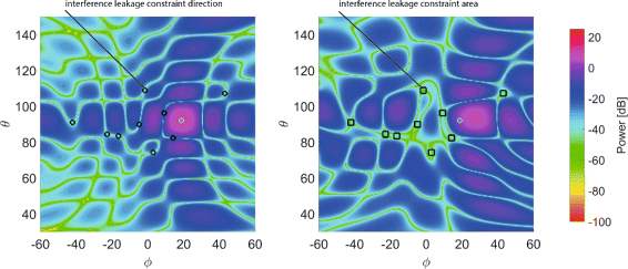
Radiation beam pattern obtained with non-robust leakage-bounded angular beamforming (left) and with robust leakage-bounded angular beamforming (right). The nine angular uncertainty regions of robust leakage-bounded angular beamforming have a width of ψ_max=±1.6° in this example
Full size image
4.
The simulation results were generated using QuaDRiGa Version 1.4.8-571.
5.
Notice, the antenna boresight direction is (ϕ,θ)= (0°,90°).
6.
Notice, for multi-user beamforming with a single stream per user we investigate the impact of the angular CSI resolution in [40] and demonstrate that an angular resolution of 4° achieves close to optimal performance for a UPA of size 10·10. Since the spatial resolution of the 50 element ULA considered here is better, we increase the angular CSI resolution to 1°.
Table 1 Simulation parameters employed to setup the QUADRIGA channel model
Full size table
7.
The definition of $\sigma _{e}^{2}$ here is slightly different as compared to (8), in order to keep the energy of the estimated channel constant irrespective of $\sigma _{e}^{2}$.

Abbreviations

3GPP:: Third generation partnership project
AD:: Analog to digital
BD:: Block diagonalization
BS:: Base station
CoMP:: Coordinated multipoint transmission
CSI:: Channel state information
CSIT:: Channel state information at the transmitter
DAS:: Distributed antenna system
DA:: Digital to analog
DoF:: Degrees of freedom
FD:: Full-dimension
FDD:: Frequency division duplex
FD-MIMO:: Full-dimension multiple-input multiple-output
FRT:: Fluctuating two-ray
GRT:: Generalized two-ray
IA:: Interference alignment
i.i.d.:: Independent and identically distributed
ITS:: Intelligent transport systems
LOS:: Line of sight
LTE:: Long term evolution
MBMS:: Multimedia broadcast multicast service
eMBMS:: Evolved MBMS
MC-IC:: Multicast interference channel
MIMO:: Multiple-input multiple-output
MISO:: Multiple-input single-output
NLOS:: Non-line of sight
NP:: Non-deterministic polynomial-time
NR:: New radio
OFDM:: Orthogonal frequency division multiplexing
OMP:: Orthogonal matching pursuit
QAM:: Quadrature amplitude modulation
RF:: Radio frequency
RRH:: Remote radio head
SDMA:: Space-division multiple access
SDR:: Semidefinite programming relaxation
SER:: Symbol error ratio
SINR:: Signal to interference and noise ratio
SLNR:: Signal to leakage and noise ratio
SLR:: Signal to leakage ratio
SNR:: Signal to noise ratio
SVD:: Singular value decomposition
TDD:: Time division duplex
TTI:: Transmission time interval
TWDP:: Two-wave diffuse power
UC-IC:: Unicast interference channel
UE:: User equipment
UMTS:: Universal mobile telecommunications system
ULA:: Uniform linear array
UPA:: Uniform planar array
ZF:: Zero forcing

References

1
H Yang, T Marzetta, Performance of conjugate and zero-forcing beamforming in large-scale antenna systems. IEEE J. Sel. Areas Commun. 31(2), 172–179 (2013).
Article Google Scholar
2
Y Kim, H Ji, J Lee, YH Nam, BL Ng, I Tzanidis, Y Li, J Zhang, Full dimension MIMO (FD-MIMO): The next evolution of MIMO in LTE systems. IEEE Wirel. Commun. 21(3), 92–100 (2014).
Article Google Scholar
3
YH Nam, MS Rahman, Y Li, G Xu, E Onggosanusi, J Zhang, JY Seol, in Information Theory and Applications Workshop (ITA). Full dimension MIMO for LTE-Advanced and 5G (IEEESan Diego, 2015), pp. 143–148.
Google Scholar
4
M Kim, YH Lee, MSE-based hybrid RF/baseband processing for millimeter-wave communication systems in MIMO interference channels. IEEE Trans. Veh. Technol. 64(6), 2714–2720 (2015).
Article Google Scholar
5
F Sohrabi, W Yu, Hybrid digital and analog beamforming design for large-scale antenna arrays. IEEE J. Sel. Topics Signal Process. 10(3), 501–513 (2016).
Article Google Scholar
6
R Rajashekar, L Hanzo, Hybrid beamforming in mm-Wave MIMO systems having a finite input alphabet. IEEE Trans. Commun. 64(8), 3337–3349 (2016).
Article Google Scholar
7
A Liu, VKN Lau, Impact of CSI knowledge on the codebook-based hybrid beamforming in massive MIMO. IEEE Trans. Signal Process. 64(24), 6545–6556 (2016).
MathSciNet Article Google Scholar
8
H Wang, W Wang, VKN Lau, Z Zhang, Hybrid limited feedback in 5G cellular systems with massive MIMO. IEEE Syst. J. 11(1), 50–61 (2017).
Article Google Scholar
9
C Rusu, R Méndez-Rial, N González-Prelcic, RW Heath, Low complexity hybrid precoding strategies for millimeter wave communication systems. IEEE Trans. Wirel. Commun. 15(12), 8380–8393 (2016).
Article Google Scholar
10
QUA Nadeem, A Kammoun, M Debbah, MS Alouini, Design of 5G full dimension massive MIMO systems. IEEE Trans. Commun. PP(99), 1–1 (2017).
Google Scholar
11
N Li, Z Wei, H Yang, X Zhang, D Yang, Hybrid precoding for mmWave massive MIMO systems with partially connected structure. IEEE Access. 5:, 2–15151 (1514).
Google Scholar
12
O Orhan, E Erkip, S Rangan, in 2015 Information Theory and Applications Workshop (ITA). Low power analog-to-digital conversion in millimeter wave systems: impact of resolution and bandwidth on performance (IEEESan Diego, 2015), pp. 191–198.
Google Scholar
13
S Jacobsson, G Durisi, M Coldrey, U Gustavsson, C Studer, Throughput analysis of massive MIMO uplink with low-resolution ADCs. IEEE Trans. Wirel. Commun. 16(6), 4038–4051 (2017).
Article Google Scholar
14
WB Abbas, F Gomez-Cuba, M Zorzi, Millimeter wave receiver efficiency: a comprehensive comparison of beamforming schemes with low resolution ADCs. IEEE Trans. Wirel. Commun. 16(12), 8131–8146 (2017).
Article Google Scholar
15
K Roth, JA Nossek, Achievable rate and energy efficiency of hybrid and digital beamforming receivers with low resolution ADC. IEEE J. Sel. Areas Commun. 35(9), 2056–2068 (2017).
Article Google Scholar
16
TE Bogale, LB Le, Massive MIMO and mmWave for 5G wireless HetNet: potential benefits and challenges. IEEE Veh. Technol. Mag. 11(1), 64–75 (2016).
Article Google Scholar
17
LN Ribeiro, S Schwarz, M Rupp, ALF de Almeida, Energy efficiency of mmWave massive MIMO precoding with low-resolution DACs. CoRR. abs/1709.05139: (2017).
18
J Zuo, J Zhang, C Yuen, W Jiang, W Luo, Multicell multiuser massive MIMO transmission with downlink training and pilot contamination precoding. IEEE Trans. Veh. Technol. 65(8), 6301–6314 (2016).
Article Google Scholar
19
Y Han, J Lee, Uplink pilot design for multi-cell massive MIMO networks. IEEE Commun. Lett. 20(8), 1619–1622 (2016).
Article Google Scholar
20
S Schwarz, R Heath, M Jr. Rupp, Single-user MIMO versus multi-user MIMO in distributed antenna systems with limited feedback. EURASIP J. Adv. Sig. Proc. 2013(1), 54 (2013).
Article Google Scholar
21
W Shen, L Dai, Y Shi, B Shim, Z Wang, Joint channel training and feedback for FDD massive MIMO systems. IEEE Trans. Veh. Technol. 65(10), 8762–8767 (2016).
Article Google Scholar
22
MS Sim, J Park, CB Chae, RW Heath, Compressed channel feedback for correlated massive MIMO systems. J. Commun. Netw. 18(1), 95–104 (2016).
Article Google Scholar
23
S Schwarz, T Philosof, M Rupp, Signal processing challenges in cellular assisted vehicular communications. IEEE Signal Process. Mag. 34(2), 47–59 (2017).
Article Google Scholar
24
MA Maddah-Ali, D Tse, Completely stale transmitter channel state information is still very useful. IEEE Trans. Inf. Theory. 58(7), 4418–4431 (2012).
MathSciNet Article MATH Google Scholar
25
S Yang, M Kobayashi, D Gesbert, X Yi, Degrees of freedom of time correlated MISO broadcast channel with delayed CSIT. IEEE Trans. Inf. Theory. 59(1), 315–328 (2013).
MathSciNet Article MATH Google Scholar
26
J Chen, P Elia, Toward the performance versus feedback tradeoff for the two-user MISO broadcast channel. IEEE Trans. Inf. Theory. 59(12), 8336–8356 (2013).
MathSciNet Article MATH Google Scholar
27
H Joudeh, B Clerckx, Sum-rate maximization for linearly precoded downlink multiuser MISO systems with partial CSIT: A rate-splitting approach. IEEE Trans. Commun. 64(11), 4847–4861 (2016).
Article Google Scholar
28
C Peel, B Hochwald, A Swindlehurst, A vector-perturbation technique for near-capacity multiantenna multiuser communication-part I: channel inversion and regularization. IEEE Trans. Commun. 53(1), 195–202 (2005).
Article Google Scholar
29
Q Spencer, A Swindlehurst, M Haardt, Zero-forcing methods for downlink spatial multiplexing in multiuser MIMO channels. IEEE Trans. Signal Process. 52(2), 461–471 (2004).
MathSciNet Article MATH Google Scholar
30
V Cadambe, S Jafar, Interference alignment and degrees of freedom of the K-user interference channel. IEEE Trans. Inf. Theory. 54(8), 3425–3441 (2008).
MathSciNet Article MATH Google Scholar
31
M Maddah-Ali, A Motahari, A Khandani, Communication over MIMO X channels: interference alignment, decomposition, and performance analysis. IEEE Trans. Inf. Theory. 54(8), 3457–3470 (2008).
MathSciNet Article MATH Google Scholar
32
J Zhang, RW Heath Kountouris, JG Andrews, Mode switching for the multi-antenna broadcast channel based on delay and channel quantization. EURASIP J. Adv. Signal Process. 2009(1), 802548 (2009).
Article MATH Google Scholar
33
S Schwarz, R Heath, Rupp Jr M, in 38th International Conference on Acoustics, Speech and Signal Processing. Adaptive quantization on the Grassmann-manifold for limited feedback multi-user MIMO systems (IEEEVancouver, 2013), pp. 5021–5025.
Google Scholar
34
SA Vorobyov, Principles of minimum variance robust adaptive beamforming design.Signal Process. 93(12), 3264–3277 (2013). special Issue on Advances in Sensor Array Processing in Memory of Alex B. Gershman.
35
WS Chua, C Yuen, YL Guan, F Chin, Robust multi-antenna multi-user precoding based on generalized multi-unitary decomposition with partial CSI feedback. IEEE Trans. Veh. Technol. 62(2), 596–605 (2013).
Article Google Scholar
36
S Schwarz, M Rupp, Evaluation of distributed multi-user MIMO-OFDM with limited feedback. IEEE Trans. Wirel. Commun. 13(11), 6081–6094 (2014).
Article Google Scholar
37
J Wang, M Bengtsson, B Ottersten, DP Palomar, Robust MIMO precoding for several classes of channel uncertainty. IEEE Trans. Signal Process. 61(12), 3056–3070 (2013).
Article Google Scholar
38
F Khalid Speidel, Robust hybrid precoding for multiuser MIMO wireless communication systems. IEEE Trans. Wirel. Commun. 13(6), 3353–3363 (2014).
Article Google Scholar
39
S Schwarz, T Philosof, M Rupp, in 50th Asilomar Conference on Signals Systems and Computers. Convex-optimization based geometric beamforming for FD-MIMO arrays (IEEEAsilomar, 2016).
Google Scholar
40
S Schwarz, M Rupp, in 50th Asilomar Conference on Signals Systems and Computers. Limited feedback based double-sided full-dimension MIMO for mobile backhauling (IEEEAsilomar, 2016).
Google Scholar
41
P Almers, E Bonek, A Burr, N Czink, M Debbah, V Degli-Esposti, H Hofstetter, P Kyösti, D Laurenson, G Matz, A Molisch, C Oestges, H Özcelik, Survey of channel and radio propagation models for wireless MIMO systems. EURASIP J. Wirel. Commun. Netw. 2007(019070), 19 (2007).
Google Scholar
42
H Özcelik, Indoor MIMO channel models, 2004 (Wien, Technische Universität, Dissertation, 2005). http://resolver.obvsg.at/urn:nbn:at:at-ubtuw:1-17999.
43
CA Balanis, Antenna theory: analysis and design, 3rd (Wiley, New Jersey, 2005).
Google Scholar
44
H Ji, Y Kim, J Lee, E Onggosanusi, Y Nam, J Zhang, B Lee, B Shim, Overview of full-dimension MIMO in LTE-advanced pro. IEEE Commun. Mag. 55(2), 176–184 (2017).
Article Google Scholar
45
J Choi, V Va, N Gonzalez-Prelcic, R Daniels, CR Bhat, RW Heath, Millimeter-wave vehicular communication to support massive automotive sensing. IEEE Commun. Mag. 54(12), 160–167 (2016).
Article Google Scholar
46
GD Durgin, TS Rappaport, DA de Wolf, New analytical models and probability density functions for fading in wireless communications. IEEE Trans. Commun. 50(6), 1005–1015 (2002).
Article Google Scholar
47
M Rao, FJ Lopez-Martinez, A Goldsmith, in 2014 48th Annual Conference on Information Sciences and Systems. Statistics and system performance metrics for the two wave with diffuse power fading model (IEEEPrinceton, 2014), pp. 1–6.
Google Scholar
48
M Rao, FJ Lopez-Martinez, MS Alouini, A Goldsmith, MGF approach to the analysis of generalized two-ray fading models. IEEE Trans. Wirel. Commun. 14(5), 2548–2561 (2015).
Google Scholar
49
JM Romero-Jerez, FJ Lopez-Martinez, JF Paris, A Goldsmith, in 2016 IEEE Globecom Workshops. The fluctuating two-ray fading model for mmWave communications (IEEEWashington, 2016), pp. 1–6.
Google Scholar
50
S Schwarz, Outage investigation of beamforming over random-phase finite-scatterer MISO channels. IEEE Signal Process. 24(7), 1029–1033 (2017).
Article Google Scholar
51
J Zhang, W Zeng, X Li, Q Sun, KP Peppas, New results on the fluctuating two-ray model with arbitrary fading parameters and its applications. IEEE Trans. Veh. Technol. PP(99), 1–1 (2017).
Google Scholar
52
E Dahlman, S Parkvall, J Sköld, 4G LTE/LTE-advanced for mobile broadband (Elsevier Academic Press, Oxford, 2011).
Google Scholar
53
O El Ayach, R Heath Jr., Grassmannian differential limited feedback for interference alignment. IEEE Trans. Signal Process. 60(12), 6481–6494 (2012).
MathSciNet Article Google Scholar
54
YC Eldar, G Kutyniok, Compressed sensing: theory and applications (Cambridge Univ. Press, Cambridge, 2012).
Google Scholar
55
YC Pati, R Rezaiifar, PS Krishnaprasad, in Proceedings of 27th Asilomar Conference on Signals, Systems and Computers. Orthogonal matching pursuit: recursive function approximation with applications to wavelet decomposition, (1993), pp. 40–44.
56
Z-Q Luo, W-K Ma, A-C So, Y Ye, S Zhang, Semidefinite relaxation of quadratic optimization problems. IEEE Signal Process. Mag. 27(3), 20–34 (2010).
Article Google Scholar
57
Z Luo, ND Sidiropoulos, P Tseng, S Zhang, Approximation bounds for quadratic optimization with homogeneous quadratic constraints. SIAM J. Optim. 18(1), 1–28 (2007).
MathSciNet Article MATH Google Scholar
58
T-H Chang, Z-Q Luo, C-Y Chi, Approximation bounds for semidefinite relaxation of max-min-fair multicast transmit beamforming problem. IEEE Trans. Signal Process. 56(8), 3932–3943 (2008).
MathSciNet Article Google Scholar
59
R Zhang, YC Liang, Exploiting multi-antennas for opportunistic spectrum sharing in cognitive radio networks. IEEE J. Sel. Topics Signal Process. 2(1), 88–102 (2008).
Article Google Scholar
60
Y Nesterov, A Nemirovski, Interior-point polynomial algorithms in convex programming: theory and applications (Philadelphia: Society for Industrial and Applied Mathematics, SIAM, 1994).
Google Scholar
61
MS Lobo, L Vandenberghe, S Boyd, H Lebret, Applications of second-order cone programming. Linear Algebra Appl. 284(1), 193–228 (1998). international Linear Algebra Society (ILAS) Symposium on Fast Algorithms for Control, Signals and Image Processing.
MathSciNet Article MATH Google Scholar
62
R Zhang, S Cui, Cooperative interference management with MISO beamforming. IEEE Trans. Signal Process. 58(10), 5450–5458 (2010).
MathSciNet Article Google Scholar
63
S Schwarz, M Rupp, Transmit optimization for the MISO multicast interference channel. IEEE Trans. Commun. 63(12), 4936–4949 (2015).
Article Google Scholar
64
Z-Q Luo, T-H Chang, in Convex Optimization in Signal Processing and Communications, ed. by D Palomar, Y Eldar. SDP relaxation of homogeneous quadratic optimization: approximation and applications (Cambridge University Press, 2010).
65
F Alizadeh, D Goldfarb, Second-order cone programming. Math Program. 95:, 3–51 (2001).
MathSciNet Article MATH Google Scholar
66
C Wang, D Sun, K-C Toh, Solving log-determinant optimization problems by a newton-cg primal proximal point algorithm. SIAM J. Optim. 20(6), 2994–3013 (2010).
MathSciNet Article MATH Google Scholar
67
YP Lin, SH Tsai, in 2017 IEEE 18th International Workshop on Signal Processing Advances in Wireless Communications (SPAWC) (Thic structures for rf beamforming, 2017), pp. 1–5.
68
Y Lee, Y Nam, J So, in 2012 18th Asia-Pacific Conference on Communications (APCC). Optimal user selection algorithm for opportunistic space division multiple access systems (IEEEJeju Island, 2012), pp. 922–923.
Google Scholar
69
HL Van Trees, Detection, estimation, and modulation theory. Part IV., Optimum array processing (Wiley-Interscience, New York, 2002).
Google Scholar
70
F-I Tseng, DK Cheng, Optimum scannable planar arrays with an invariant sidelobe level. Proc IEEE. 56(11), 1771–1778 (1968).
Article Google Scholar
71
N Jindal, MIMO broadcast channels with finite-rate feedback. IEEE Trans. Inf. Theory. 52(11), 5 (2006).
MathSciNet Article MATH Google Scholar
72
N Ravindran, N Jindal, Limited feedback-based block diagonalization for the MIMO broadcast channel. IEEE J. Sel. Areas Commun. 26(8), 1473–1482 (2008).
Article Google Scholar
73
S Schwarz, M Rupp, Subspace quantization based combining for limited feedback block-diagonalization. IEEE Trans. Wirel. Commun. 12(11), 5868–5879 (2013).
Article Google Scholar
74
X Zhang, J Tadrous, E Everett, F Xue, A Sabharwal, in 2015 49th Asilomar Conference on Signals, Systems and Computers. Angle-of-arrival based beamforming for FDD massive MIMO, (2015), pp. 704–708.
75
M Sadek, A Tarighat, A Sayed, A leakage-based precoding scheme for downlink multi-user MIMO channels. IEEE Trans. Wirel. Commun. 6(5), 1711–1721 (2007).
Article Google Scholar
76
S Jaeckel, L Raschkowski, K Börner, L Thiele, Quadriga: A 3-D multi-cell channel model with time evolution for enabling virtual field trials. IEEE Trans. Antennas Propag. 62(6), 3242–3256 (2014).
Article Google Scholar
77
M Grant, S Boyd, CVX: Matlab software for disciplined convex programming, version 2.1. (2014). http://cvxr.com/cvx.
78
H Xie, F Gao, S Zhang, S Jin, A unified transmission strategy for TDD/FDD massive MIMO systems with spatial basis expansion model. IEEE Trans. Veh. Technol. 66(4), 3170–3184 (2017).
Article Google Scholar

Download references

Acknowledgements

The financial support by the Austrian Federal Ministry of Science, Research and Economy and the National Foundation for Research, Technology and Development is gratefully acknowledged. The author acknowledges the TU Wien University Library for the financial support through its Open Access Funding Program.

Funding

Not applicable.

Availability of data and materials

Not applicable.

Author information

Affiliations

Christian Doppler Laboratory for Dependable Wireless Connectivity for the Society in Motion, Institute of Telecommunications, Technische Universität (TU) Wien, Vienna, Austria
Stefan Schwarz

Authors

Stefan Schwarz
View author publications
You can also search for this author in PubMed Google Scholar

Contributions

All contributions are from the sole author SS. The author read and approved the final manuscript.

Corresponding author

Correspondence to Stefan Schwarz.

Ethics declarations

Competing interests

The author declares that he has no competing interests.

Publisher’s Note

Springer Nature remains neutral with regard to jurisdictional claims in published maps and institutional affiliations.

Additional information

Authors’ information

Not applicable.

Rights and permissions

Open Access This article is distributed under the terms of the Creative Commons Attribution 4.0 International License (http://creativecommons.org/licenses/by/4.0/), which permits unrestricted use, distribution, and reproduction in any medium, provided you give appropriate credit to the original author(s) and the source, provide a link to the Creative Commons license, and indicate if changes were made.

Reprints and Permissions

About this article

Cite this article

Schwarz, S. Robust full-dimension MIMO transmission based on limited feedback angular-domain CSIT. J Wireless Com Network 2018, 58 (2018). https://doi.org/10.1186/s13638-018-1070-0

Download citation

Received: 09 August 2017
Accepted: 23 February 2018
Published: 14 March 2018
DOI: https://doi.org/10.1186/s13638-018-1070-0

Keywords

Full-dimension MIMO
3D beamforming
Robust precoding
Interference leakage
High mobility
Limited feedback

Robust full-dimension MIMO transmission based on limited feedback angular-domain CSIT

Abstract

Introduction

System model

Channel model

Transmission model

Targeted deployment scenarios

Channel state information feedback

Leakage-bounded angular beamforming and precoding

Leakage-bounded angular beamforming

Leakage-bounded angular precoding

Implementation issues

Computational complexity

Combination with hybrid architectures

Benchmark methods

Interference-unaware beamsteering

Max-gain beamsteering

Chebyshev-tapered beamsteering

Interference-aware precoding

Block-diagonalization precoding

Angle of departure block-diagonalization precoding

Hybrid block-diagonalization precoding

Incoherent SLNR precoding

Simulations

Radiation beam pattern

Comparison to interference-unaware beamsteering

Comparison to interference-aware precoding

Conclusions

Appendix

Upper bound on the approximation \(\hat {\tilde {R}}_{u}\)

Notes

Abbreviations

References

Acknowledgements

Funding

Availability of data and materials

Author information

Affiliations

Contributions

Corresponding author

Ethics declarations

Competing interests

Publisher’s Note

Additional information

Authors’ information

Rights and permissions

About this article

Cite this article

Keywords