- Research
- Open access
- Published:
TDOA versus ATDOA for wide area multilateration system
EURASIP Journal on Wireless Communications and Networking volume 2018, Article number: 179 (2018)
Abstract
This paper outlines a new method of a location service (LCS) in the asynchronous wireless networks (AWNs) where the nodes (base stations) operate asynchronously in relation to one another. This method, called asynchronous time difference of arrival (ATDOA), enables the calculation of the position of the mobile object (MO) through the measurements taken by a set of non-synchronized fixed nodes and is based on the measurement of the virtual distance difference between the reference nodes and the several MO positions (more than two), as well as on the solution of a nonlinear system of equations. The novelty of the proposed solution is using the measurements taken by at least five ground sensors without time synchronization between them to estimate the position of the tracked MO transmitting four or more sounding signals in random time.
The new method significantly simplifies the localization process in real-life AWNs. It can be used on its own or to complement the traditional synchronous method. The paper focuses on the description of the proposed ATDOA method, two algorithms TS-LS (Taylor series least-squares) and GA (genetic algorithm) for solving the nonlinear system of equations, example application of the new method for a three-dimensional space, and presentation of the simulation models and simulation results. An important part of the paper is the comparison of the efficiency between the asynchronous method and the synchronous one for wide area multilateration (WAM) system. In addition, the Cramér-Rao lower bound (CRLB) is derived for this problem as a benchmark. The preliminary measurement results obtained by applying the proposed ATDOA method against the background of the synchronous one are presented at the end of the paper. As it could be expected, the synchronous solution gives better results. The synchronous method allows to locate the aircraft within 15 m in about 80% of the time, while the ATDOA method in 74% of the time for the base stations clocked from the reference clocks with the stability equal to 10−9, and in 58% of the time for the base stations clocked from the reference clocks with the stability equal to 10−8. The new method therefore should not be treated as the improvement of the existing synchronous positioning systems but as a backup solution which allows to keep the LCS systems running even during ground stations synchronization failure.
1 Introduction
Radio positioning can be defined as a method of determining the coordinates of a radio device (object) using the properties of radio waves. Various methods have been developed over the years, including the measurements of angle of arrival (AOA), time of arrival (TOA), time difference of arrival (TDOA), and received signal strength (RSS).
The architecture of positioning systems is based on fixed nodes (base stations) and mobile objects (mobile terminals), the location of which is required [1]. In a wireless network, it is often interesting to determine the position of an object by its emission. In that case, the wireless network carries out the measurements and makes position calculations (network-based positioning) [2]. A critical aspect of a network-based positioning system is precise synchronization of the fixed nodes between one another. Synchronization systems in wireless networks are rather expensive and complicated in their architectures. Moreover, bad synchronization leads to significant errors in the positioning of objects. Therefore, the paper presents a comparison of two methods: a synchronous TDOA and an asynchronous one, where the nodes operate asynchronously in relation to one another.
The proposed asynchronous method [3], which was called asynchronous time difference of arrival (ATDOA), is based on the measurement of the time difference of arrival between the mobile object (MO) and the same set of fixed nodes at different times and on the solution of a nonlinear system of equations.
Several research groups have been working to develop asynchronous localization systems. In [4], the location system consists of distributed and autonomous sensors at some fixed and known position. The position of the object which emits some designed and known signal was estimated in that system. Sensors process the received signal (pulses) independently and send the observation results to a master station to estimate the position of that object. The master station knows the expected interval between the successive pulses and considers only pairs of pulses received from each sensor. Vaghefi [5] described asynchronous wireless source localization using TOA measurements where the source transmit time is unknown. The TOA measurements have a positive bias due to the synchronization error which could lead to a large localization error. This work presents asynchronous TOA-based source localization using a semidefinite programming (SDP) technique. The SDP is a form of convex optimization which, unlike the nonconvex maximum likelihood estimator, does not have convergence problems [6, 7]. We can find another approach in [8]. The asynchronous TDOA used time difference of arrival from a set of base stations and the interval of radar scanning between the master station and slave stations to determine the location of the target. In that system, one master station and three slave stations constituted a passive surveillance system. In turn, [9] described several reference-free localization estimators based on the TOA measurements for a scenario where the anchor nodes are synchronized and the clock of the target node runs freely. The systems described in [10,11,12,13,14,15] are a different group of solutions. All these systems rely on a two-way transmission and/or require additional reference (special) node. The ATDOA proposed in this article is a totally passive method, i.e., the transmission takes place only in one direction from the MO to fixed nodes, and all fixed nodes in the wireless network are identical.
The novelty of the paper is that the process of the asynchronous location of a moving object is based on measuring the virtual distance difference between the reference nodes and the several MO positions using four or more sounding signals transmitted by the MO in random time.
This paper is organized as follows: Section 2 describes the ATDOA method, and the next two sections present an algorithm for calculating the position of the mobile object and the simulation results respectively. Section 5 outlines the application of the ATDOA method for the WAM system together with a comparison between the synchronous and asynchronous method. Section 6 derives the Cramér-Rao lower bound (CRLB) for this problem as a benchmark, while Section 7 presents the preliminary measurement results of aircraft position estimation obtained by using the proposed ATDOA method. Finally, the last section concludes the paper.
2 Description of the proposed ATDOA method
Let us assume that N fixed nodes acting as ATDOA sensors are deployed in a wireless network, in a three-dimensional space, (Fig. 1). In general, moving objects work to the rhythm of their own clocks; therefore, it can be assumed that the moments of sending location signals from many MOs are not correlated with each other. Moreover, all objects transmit location signals with a different repetition time. The system can track multiple objects if the fixed nodes can separate the signals transmitted by each object. For simplicity, this paper focuses on a single signal source (object). The mobile object (terminal) transmits radio impulses with the unknown repetition time (Δtk), which may be even randomly variable. In the examined case, the wireless network works in an asynchronous manner—the measurement nodes are not synchronized with one another. All nodes in the network take measurements in the rhythm of their own clocks. Each node measures the so-called virtual distance difference Di,k between M observation times (in the case of five fixed nodes at least M = 4 measurements taken by each node are required for the 3D positioning)
where v is the signal propagation speed and di,k represents the distance difference of arrival between itself and the mobile object at the observation time k and k + 1 (hence, the name of the proposed method—asynchronous time difference of arrival, i.e., ATDOA [3]) and can be described as follows:
where ti,k and ti,k + 1 denote the times of the signal propagation from the mobile object (MO) to the nodes Si at the observation time k and k + 1, (Xi, Yi, Zi) represent the coordinates of the sensors, (xk, yk, zk) and (xk + 1, yk + 1, zk + 1) are the coordinates of the MO at the observation time k and k + 1 respectively. At this point, it is worth stressing that di,k physically represents the distance difference of arrival between the ith sensor and the MO at the observation time k and k + 1 (see Fig. 1 for comparison with the TDOA method), and variable Di,k is the virtual distance difference, because in addition to di,k, the sensor Si will measure the virtual distance that the radio wave will travel during the time of the MO movement from position (xk, yk, zk) to position (xk + 1, yk + 1, zk + 1).

Graphical representation of the problem under consideration
These results can be used to calculate the geographical position of the mobile object. The illustration of timing for the considered case is shown in Fig. 2. However, we must assume that we know:
-
The coordinates of fixed nodes Si,
-
The virtual distance differences between Si and the MO (Di,k) at the observation time k and k + 1 which are measured by the fixed nodes,
whereas the unknowns are:
-
The coordinates of the tracked object MO (xl, yl, zl) at the observation time l = 1, …, M,
-
The repetition time of the radio impulses which are transmitted by the mobile object (Δtk).
Fig. 2 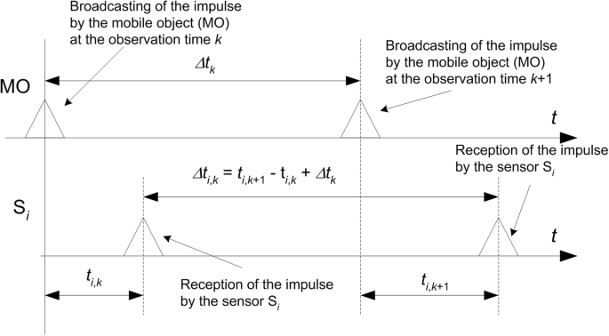
Illustration of the timing of the problem under consideration

Each node in Fig. 1 transmits the results of the measurements of the time differences Δti,k to the computing unit (CU). The transmission between the nodes and the CU which can be based on the wired or wireless link is asynchronous. The computing unit does not make any measurements but uses the results of the measurements taken by the ground sensors; therefore, the data transmission delay between the ground nodes and CU is negligible. The CU can estimate the positions of the mobile object at the observation time l, because the results of the measurements received from the fixed nodes have an MO identifier and are numbered.
In summary, the proposed method leads to establishing the coordinates of the mobile object (xl, yl, zl) and indirectly the repetition times (Δtk). In order to achieve so, assuming that N = 5 and M = 4, one must solve a system of Eq. (1) with 15 unknowns (12 coordinates of the MO in a three-dimensional space in 4 consequent measurements and 3 repetition times). Of course, in a two-dimensional space (N = 4 and M = 3), four nodes and three observation times are enough and (1) has only eight unknowns. The final part of this section emphasizes the difference between the proposed method and the solution described in [3]. The method presented in [3] requires more measurement nodes than the solution proposed in this paper. The process of asynchronous location of a moving object in the method [3] is based on measuring the virtual distance difference between the reference nodes and the MO in only two distinct positions. In the method proposed herein, these measurements are taken between the reference nodes and several positions of the MO (more than two). By using the measurements obtained from several positions of the MO, we can reduce the minimum number of the required fixed stations in the 3D case to five. Furthermore, in the proposed method, the pulse repetition time may be variable and even unknown, which means that the Δt1 does not have to be equal to Δt2, the Δt2 does not have to be equal to Δt3, etc.
3 Calculating the position of the mobile object
Solving the above-mentioned nonlinear equations is difficult. Classical methods, such as those proposed in [16], do not lead to a correct solution. This paper describes two methods of obtaining a solution of the nonlinear system of equations: an iterative algorithm based on the Taylor series least-squares (TS-LS) and a genetic algorithm (GA).
3.1 Taylor series least-squares algorithm for calculating the position of the MO
Linearizing (1) by the Taylor series expansion and then solving it iteratively is one possible way to obtain the estimates of the MO coordinates [17, 18]. The components of the n-dimensional vector x to be estimated are the position coordinates and the repetition times (indirect Δdk) in two dimensions (n = 8) or three dimensions (n = 15). Therefore, a set of N·(M − 1) measurements dp, p = 1, 2, …, N·(M − 1) is collected. In the absence of random measurement errors, dp is equal to a known function of the coordinates and the repetition time in x, which may be denoted as fp(x). In the presence of additive errors, denoted as qp
these N·(M − 1) independent Eq. (3) can be written as a single equation for the N·(M − 1)-dimensional column vector:
The measurement error q is assumed to be a multivariate random vector with the N·(M − 1) × N·(M − 1) positive-definite covariance matrix.
where E[] denotes the expected value. The f(x) is a nonlinear vector function. To determine a reasonably simple estimator, f(x) can be linearized by expanding it in a Taylor series about a reference point specified by the vector x0 and considering only the first two terms:
where x and x0 are n × 1 column vectors, and G is the N·(M − 1) × n matrix of derivatives evaluated at x0. In our case, for n = 15, the solution algorithm starts with an initial position guess x0 and computes positioning deviations
where [19]
Di,krepresents the measured values of the virtual distance differences of arrival between each node and the mobile object during the collection time. The values ri,k and ri,k + 1 are computed from (2) with x = x0. In the next iteration, x is then set to x0 − Δx. The whole process is repeated again until Δx is sufficiently small.
3.2 Genetic algorithm for calculating the position of the MO
Genetic algorithms are adaptive heuristic search algorithms based on the mechanics of a natural selection and genetics. The concept of GAs is designed to simulate processes in nature that are necessary for evolution. They loosely reflect the phenomena related to chromosomes, genes, and the evolutionary passing of a genetic material from one generation to another. The GAs do not always converge to the true minimum in a search problem. The strength of GAs is that they mostly converge rapidly to a near-optimal solution [3, 20]. The proposed genetic algorithm, which has been implemented, is as follows:

The results of numerical calculations are presented next. These calculations were carried out in order to estimate the effectiveness of solving nonlinear equations using the above methods for the asynchronous network.
4 Asynchronous multilateration system for aircraft position tracking
The proposed asynchronous method of position estimation using free-running sensors may be useful to create instances of ubiquitous positioning technology [21]. It can be applied physically to find the coordinates of mobile nodes in radio and non-radio applications. This chapter shows an example application of the ATDOA method in a three-dimensional test environment.
Currently, there are many systems available for aircraft navigation and position estimation. One of them is a wide area multilateration (WAM) system. The WAM is a technology for determining the position of an emitter (e.g., an aircraft transponder) by measuring the time difference of arrival of a signal between several known observation points [22]. In general, the majority of the WAM systems in the world utilize signals from the onboard transponders of the secondary surveillance radar (SSR) system. The SSR consists of a ground component (radar) and an airborne component (transponder) on board in an aircraft. The radar emits a signal (at 1030 MHz) which triggers a response from the airborne transponder (at 1090 MHz). A critical aspect of a working WAM system is precise synchronization of the ground stations with each other [22]. The asynchronous system presented in [23] would require the cooperation of the SSR radar to trigger emission from onboard transponders in a defined interval. The ATDOA method proposed in this paper is completely passive. It is based on the reception of broadcast signals from an airborne transponder. The time between transmissions of signals from the aircraft should be assumed as unknown and variable (irregular). Therefore, various sources of radio signals from onboard transmitters may be used for position estimation using the asynchronous multilateration system (MLAT), such as SSR, an automatic dependent surveillance-broadcast (ADS-B), or even distance measuring equipment (DME) pulses.
The experiments were carried out by using the simulation model shown in Fig. 3. To get results corresponding to the actual conditions, the choice of the coordinates of the nodes was based upon the real sites selected as candidates for the WAM system designed as a backup to the secondary radar in the terminal maneuvering area (TMA) of Gdansk airport (EPGD) in northern Poland. During all simulations, the positions of the tracked aircraft were generated randomly with a uniform distribution of the longitude in the range between 16° and 22.1° E, the latitude between 53.1° and 54.9° N, and the altitude above WGS84 geoid between 3000 and 15,000 m. In spatially incoherent noise fields of the identical receiver noise power spectra, the covariance matrix Q in (7) can be simplified to [24].

Simulation model for testing the asynchronous WAM system
The asynchronous wireless network simulator in the MATLAB environment has been developed to verify the solution. To obtain reality-reflecting results, all simulations included time measurement errors that were modeled by using a random variable with Gaussian distribution generated using MATLAB function randn:
As it is already known, four sets of object coordinates are obtained as a result of the calculation made by using the proposed ATDOA method. Therefore, comparing the proposed method with other methods focuses on the estimation of the MO position only on the basis of the last set of coordinates, i.e., for l = M. In the WAM system, the asynchronous ATDOA method was compared with the synchronous TDOA method. Both a genetic algorithm (GA) and an iterative algorithm (IA) were used to estimate the position of the mobile object in the TDOA method. The GA algorithm is based on the algorithm described in Section 3.2, while the IA is based on the Taylor series expansion and iterative calculations [17]. In our case x = xl, y = yl, and z = zl, the TDOA solution algorithm starts with an initial position guess s0 = (x0, y0, z0) and computes positioning deviations
where
The values ri (for i = 1, 2, …, N) defined in [17] are computed with s = s0, and rt_1 (for t = 2, 3, …, N) represent the measured distance differences between the reference sensor and the adjacent sensors. In the next iteration, s is then set to s0 + Δx. The whole process is repeated again until Δx is sufficiently small. As in the previous method, the errors in distance differences (rt_1) were taken into account by using the Gaussian model:
The simulation results for the WAM system are presented in the next section.
5 Simulation results
The analysis of the termination threshold of the TS-LS algorithm was performed before the simulation investigations. That is why, numerical calculations of the error resulting from rejecting high order components of the Taylor series in this algorithm were carried out. Bearing in mind (6), the full expansion of the f(x) function into the Taylor series can be written in the following form
where Δx = x − x0 and x0 represents the actual coordinates of the object, and δT is the remainder (error) from the expansion into the Taylor series. After simple transformations, this error can be described as
The above expression and the model from Fig. 3 were used for numerical calculations of the mean value from the norm of δT vector as a function of the absolute value Δx for 10,000 attempts. The flight speed of the aircraft was 250 m/s. The results of these calculations are shown in Fig. 4. From this graph, it is possible to unambiguously deduce the threshold for the stop condition of an algorithm, which is limited by the maximum permissible error of developing the positional function f(x) in the Taylor series. For example, this threshold should be no higher than 0.0013 for the expected accuracy of the location estimation of the object equal to ± 5 m. However, setting the threshold value considerably lower than presented above may increase the number of iterations without any significant improvement in the accuracy of the position estimation. During the simulation process, we calculate the mean errors (ME) [25]—separately for the x, y, and z, mean square errors (MSE)—resultant and separately for the x, y, and z, and root mean square errors (RMSE)—resultant and separately for the x, y, and z on the basis of the average of 10,000 independent runs (Table 1). The parameters of the genetic algorithm were as follows: W = 1024, thold = 0.1 μs, and n_iter = 5000. As before, it is also assumed that the plane was moving at a speed of 250 m/s (900 km/h). The time between transmissions of the signals from the aircraft transponder was modeled as a random variable with a uniform distribution in the range from 0.25 to 2 s, while the initialization vector in the iterative and the genetic algorithm was selected randomly in the expected solution space. The accuracy of the position estimation depends on the parameter ε (εTDOA = εATDOA = ε) which represents the precision of the measured distance differences, and partially on the position of mobile node in the simulated area. The impact of the last factor was reduced by averaging the results obtained by using different, randomly chosen coordinates of the aircraft during the simulation. The genetic algorithm outperformed the iterative Taylor series based one in both TOA and TDOA simulations. For ε = 100 m, the iterative algorithm for ATDOA method did not find solutions at all. The above leads to the conclusion that the algorithm is sensitive to measurement errors. Moreover, simulation tests confirmed the possibility that the position of the object cannot be calculated, as the proposed iterative algorithm might not return a value in two cases:
-
The result of the computation is a complex number,
-
The result does not lie in the area of interest.

The mean value from the norm of δT vector as a function of the absolute value Δx
In turn, the genetic algorithm always leads to a solution, even if it is not correct (e.g., due to convergence to some local minima of ||f(x0)|| instead of a global one). The research results of the test conducted in the three-dimensional simulation environment presented here prove that the proposed method is an effective alternative to synchronous solutions.
The cumulative probability distribution function (CDF) of absolute position errors Δr, expressed in the following equations, was obtained in the next stage of the simulation studies
where xl, yl, and zl represent the real coordinates of the mobile object, and \( {\widehat{x}}_l \), \( {\widehat{y}}_l \), and \( {\widehat{z}}_l \) denote the estimated coordinates of the mobile object. The simulation results are shown in Figs. 5 and 6. Figure 5 summarizes the efficiency of the iterative algorithms, while Fig. 6 the efficiency of the genetic algorithms. Of course, the accuracy of object positioning depends on the method and the algorithm used to solve the nonlinear equations. Fundamentally, the synchronous method gives better results. However, the performance of the proposed asynchronous position estimation method may be sufficient for many applications. In some cases, the ATDOA method has even better results than the TDOA one. For example, the aircraft is located within 150 m in about 50% of the time when the TDOA method is applied (the iterative algorithm and ε = 10 m) and in 41% of the time while using the ATDOA method also for the TS-LS. On the other hand, the airplane is located within 100 m in 45% of the time while applying the TDOA method (genetic algorithm and ε = 10 m) and in 96% of the time through the ATDOA method also for GA and for ε = 10 m.
It turns out that the genetic algorithms for solving the nonlinear system of equations are more efficient in comparison with the iterative, especially for large values of measurement errors and a limited number of iterations.

The CDFs of the absolute position error for the proposed ATDOA method compared with the TDOA method using iterative algorithms TS-LS and IA respectively

The CDFs of the absolute position error for the proposed ATDOA method compared with the TDOA method using genetic algorithms
The accepted values of position estimation errors for WAM systems are not frequently discussed in the literature. However, in [26, 27], the accuracy of 0.1 NM is mentioned as satisfactory for the aircraft surveillance systems with 3 and 5 NM separation between planes, so one can assume that the values of the position estimation error reaching the size of the aircraft (tens of meters) is acceptable in most applications. Hence, the comments about the obtained results are related to this assumption.
At the end of this section, it is also worth considering the convergence of the algorithms used to solve the system of the nonlinear equations. In Fig. 7, we plot the changes in the norm of the navigation equation ||f(x0)||. As it was to be expected, the convergence of the algorithms depends on the error of measuring the virtual distance difference. For small values of ε, the curves in Fig. 7 quickly decrease to 0 for TS-LS. To reach a given convergence threshold, we need from a few to a dozen iteration numbers. In turn, for large values of ε, the TS-LS the algorithm shows large fluctuations in the value of the norm function depending on the number of iterations. Due to these large variations, this algorithm may not find practical applications for relatively large ε values. These disadvantages do not occur in a genetic algorithm, but its convergence is much slower than the TS-LS. The decrease in the value of the norm function for GA is similar to the TS-LS. However, after a certain number of iterations, the norm value stabilizes at a constant level (convergence threshold), and further repetitions of the genetic algorithm do not cause significant changes in the norm value. For obvious reasons, the higher the error values of the ε, the greater the convergence threshold.

Norm of navigation equation as a function of a number of iteration for a different algorithm
To sum up, the proposed method gives quite good results and significantly simplifies the localization process in the multilateration system. In addition, the ATDOA method does not need the round trip time (RTT) measurement, as compared with the solution in [23, 28]. Moreover, the proposed method can be applied to track unmanned aerial vehicles (UAV) [29], commonly known as drones. Tracked drones should only transmit control signals which, to hide their identities, do not have to be repeated at a constant frequency or contain any repetitive identifier. On the other hand, the development of the asynchronous method is not meant to compete with the synchronous one but to ensure the continuity of the location service (LCS) services in the WAM system. Therefore, the new method should be treated as a backup solution which allows access to the LCS service during a failure of the synchronous system.
6 Cramér-Rao lower bound
It is well known that the variance of an unbiased estimator \( \widehat{\theta} \) is bounded below by the Cramér-Rao lower bound (CRLB). The CRLB for a scalar parameter is given by [30].
where the derivative is evaluated at the true value of θ, and the expectation is taken with respect to a probability density function p(x; θ). The vector parameter CRLB will allow us to place a bound on the variance of each element. The variance of any unbiased estimator \( \widehat{\theta} \) must satisfy
where I(θ) is the Fisher information matrix which is given as
For the Gaussian error distribution case, this matrix can be expressed as [4].
where G(θ) is the Jacobian matrix described by (9), and the matrix Q is represented by (11).
Using the above expressions, we calculate the CRLB of the position estimate in the x, y, and z coordinates for both synchronous TDOA and asynchronous ATDOA systems, as a function of the aircraft speed. It was assumed in the calculations that the location of the object established by using the ATDOA method is determined by the coordinates (x10, x11, x12), i.e., the MO coordinates (x, y, z) at the moment of observation for M = 4. The obtained results were collected for 10,000 random positions of the object in the studied area and are shown in Fig. 8. The analysis of the results obtained by applying the ATDOA method shows that for the speed of the aircraft reaching 250 m/s (a typical flight speed of commercial planes), the root mean square (RMS) error is not higher than 100 m, with a further reduction to approx. 70 m for a higher speed of military planes. This demonstrates the good location performance of the proposed method for the WAM system using the asynchronous method with only five ground-based sensors. The RMS error for the synchronous method is about 10 m.

RMS CRLB for coordinates versus the speed of the aircraft
7 ATDOA measurement experiment
In this section, we present the results of the experiments carried out using the installation of an experimental synchronous WAM system located in the vicinity of one of the Polish airports (Fig. 9). Four measurement nodes were placed (red triangles) around the runway in the area of the aerodrome. The tracked aircraft was moving along the taxiways at the airport (the 2D case), and during that movement, several tens of ADS-B (automatic dependent surveillance-broadcast) messages were being recorded and processed by the WAM receivers giving reference (“true”) coordinates of the aircraft presented in Fig. 9 (the black rhombus). The geographical coordinates are given in the UTM (Universal Transverse Mercator) system. Each measurement node was synchronized using a simple GPS (Global Positioning System) receiver with a short-term clock stability at level ετ = 10−7. In order to analyze the work of the asynchronous solution, the ATDOA algorithms presented in this paper were used to process the data from the synchronous WAM receivers marked with the GPS timestamps. Unfortunately, the analyses indicated that the stability of 10−7 was insufficient for the ATDOA method. In order to estimate the efficiency of the proposed method, the measurements’ data were re-processed using the measurement noise models for the stability of 10−8 and 10−9 (the gray circle) [31]. The CDF of absolute position errors was calculated (Fig. 10) for the considered scenario. The results obtained through the asynchronous method were compared with the synchronous ones. The ATDOA equations for the considered two-dimensional case of the taxiing aircraft were solved using the genetic algorithm described in Section 3.2. As we would expect, the synchronous solution gives better results compared with the asynchronous one. For example, the aircraft is located within 15 m in about 80% of the time by using the TDOA method and in 74% of the time through the ATDOA method for ετ = 10−9 and in 58% of the time for ετ = 10−8.

Illustration of the considered case for testing the asynchronous solution

The CDFs of the absolute position error for the proposed ATDOA method compared with the TDOA method using genetic algorithms during the experiment
8 Conclusions
The paper presents a new position estimation method called ATDOA, based on the virtual distance differences between the reference nodes and several positions of the mobile object (more than two), which is dedicated to asynchronous wireless networks, especially for the application in the WAM system.
In order to estimate the position of objects, the new method requires at least one more reference node than the synchronous solutions. Simulation studies of the new method in the 3D test environments were conducted providing satisfactory results every time. For example, the aircraft is located within 100 m in about 96% of the time by using the ATDOA method for the genetic algorithm and for the distance measurement error ε = 10 m.
This method can be used on its own or to complement the typical position estimation algorithms in synchronous systems in the case of the node synchronization failure. The disadvantage of this method resulting from the iterative algorithm or the genetic algorithm is the fact that it does not always lead to the best solution due to the possibility of convergence to the incorrect local minimum of the target function. However, studies show that it happens relatively rarely and can be detected by, e.g., tracking the position estimates by using the consecutive measurements.
References
K Yu, I Sharp, YJ Guo, Ground-based wireless positioning (Wiley, UK, 2009)
A Küpper, Location-based services. Fundamentals and operation (Wiley, England, 2005)
J Stefanski, Asynchronous time difference of arrival (ATDOA) method. Pervasive Mob Comput. (2014). https://doi.org/10.1016/j.pmcj.2014.10.008
T Li, YF Huang, A location system using asynchronous distributed sensors. Twenty-third Annual Joint Conf IEEE Comp Commun Soc (INFOCOM) (2004). https://doi.org/10.1109/INFCOM.2004.1354533
RM Vaghefi, RM Buehrer, Asynchronous time-of-arrival-based source localization. IEEE Int Conf Acoust, Speech Signal Process (ICASSP) (2013). https://doi.org/10.1109/ICASSP.2013.6638427
K Yang, G Wang, ZQ Luo, Efficient convex relaxation methods for robust target localization by a sensor network using time differences of arrivals. IEEE Trans. Signal Process. (2009). https://doi.org/10.1109/TSP.2009.2016891
E Xu, Z Ding, S Dasgupta, Source localization in wireless sensor networks from signal time-of-arrival measurements. IEEE Trans. Signal Process. (2011). https://doi.org/10.1109/TSP.2011.2116012
D Zhou, X Wang, Y Tian, Airborne asynchronous TDOA based on critical area. IEEE Int Conf Comput Inf Tech (2014). https://doi.org/10.1109/CIT.2014.32
Y Wang, G Leus, Reference-free time-based localization for an asynchronous target. EURASIP J Adv Signal Process. (2012). https://doi.org/10.1186/1687-6180-2012-19
T Sathyan, D Humphrey, M Hedley, WASP: a system and algorithms for accurate radio localization using low-cost hardware. IEEE Trans. Syst. Man Cybern. Part C Appl. Rev. (2011). https://doi.org/10.1109/TSMCC.2010.2051027
B Xu, G Sun, R Yu, Z Yang, High-accuracy TDOA-based localization without time synchronization. IEEE Trans Parallel Distrib Syst. (2013). https://doi.org/10.1109/TPDS.2012.248
M Youssef, A Youssef, C Rieger, U Shankar, A Agrawala, PinPoint: an asynchronous time-based location determination system. Proc 4th Int Conf Mob Syst, Appl Serv (2006). https://doi.org/10.1145/1134680.1134698
Y Wang, G Leus, X Ma, Time-based localization for asynchronous wireless sensor networks. IEEE Int Conf Acoust, Speech Signal Process (ICASSP) (2011). https://doi.org/10.1109/ICASSP.2011.5946723
H Xiong, Z Chen, W An, B Yang, Robust TDOA localization algorithm for asynchronous wireless sensor networks. Int J Distrib Sen Net. (2015). https://doi.org/10.1155/2015/598747
H Nawaz, A Bozkurt, I Tekin, A novel power efficient asynchronous time difference of arrival indoor localization system using CC1101 radio transceivers. Microw. Opt. Technol. Lett. (2017). https://doi.org/10.1002/mop.30342
J Stefanski, Low cost method for location service in the WCDMA system. Nonlinear Anal: Real World Appl. (2013). https://doi.org/10.1016/j.nonrwa.2012.07.022
WH Foy, Position-location solutions by Taylor-series estimation. IEEE Trans. Aerosp. Electron. Syst. (1976). https://doi.org/10.1109/TAES.1976.308294
DJ Torrieri, Statistical theory of passive location systems. IEEE Trans. Aerosp. Electron. Syst. (1984). https://doi.org/10.1109/TAES.1984.310439
J Stefanski, New method of locating mobile terminal in asynchronous cellular Networks, Electronics - Designs, Technologies and Applications, No. 9 (2007), pp. 56–58 (in Polish)
CL Karr, B Weck, LM Freeman, Solutions to systems of nonlinear equations via a genetic algorithm. Eng. Appl. Artif. Intell. (1998). https://doi.org/10.1016/S0952-1976(97)00067-5
R Mannings, Ubiquitous positioning (Artech House, USA, 2008)
M Pelant, V Stejskal, in Tyrrhenian International IEEE Workshop on Digital Communications–Enhanced Surveillance of Aircraft and Vehicles. Multilateration system time synchronization via over-determination of TDOA measurements (2011), pp. 179–183
J Stefanski, Asynchronous wide area multilateration system. Aerosp. Sci. Technol. (2014). https://doi.org/10.1016/j.ast.2014.03.016
YT Chan, KC Ho, A simple and efficient estimator for hyperbolic location. IEEE Trans. Signal Process. (1994). https://doi.org/10.1109/78.301830
MH Hayes, Statistical digital signal processing and modeling (Wiley, USA, 1996)
Thompson S. D., Andrews J. W., Harris G. S., Sinclair K. A., Required surveillance performance accuracy to support 3-mile and 5-mile separation in the National Airspace System, Project Report ATC-323, Lincoln Laboratory, 2006.
Guidance Material On Comparison Of Surveillance Technologies (GMST), International Civil Aviation Organization Asia and Pacific, Edition 1.0, 2007.
J Stefanski, Simplified algorithm for location service for the UMTS. Proc IEEE 62nd Veh Techn Conf (2005). https://doi.org/10.1109/VETECF.2005.1559048
PB Sujit, S Saripalli, J Borges Sousa, Unmanned aerial vehicle path following: a survey and analysis of algorithms for fixed-wing unmanned aerial vehicles. IEEE Control. Syst. Mag. (2014). https://doi.org/10.1109/MCS.2013.2287568
SM Kay, Fundamentals of statistical signal processing—estimation theory (Prentice Hall, USA, 1993)
Operation and service manual, FS725 rubidium frequency standard, Version 1.1 (Stanford Research Systems, USA, 2005)
Acknowledgements
The authors would like to thank AVIONIX ENGINEERING sp. z o. o. for providing the measurement results.
Funding
This work is supported by the Polish National Centre for Research and Development under grant number POIR.04.01.04-00-0032/16.
Availability of data and materials
The measurement data, which were used during our investigations, are the property of AVIONIX ENGINEERING sp. z o. o.
Author information
Authors and Affiliations
Contributions
Both authors contributed to this work, and they jointly proposed a new localization method. JSt performed the experiments, while JSt and JSa analyzed the results. Both authors read and approved the final manuscript.
Corresponding author
Ethics declarations
Competing interests
The authors declare that they have no competing interests.
Publisher’s Note
Springer Nature remains neutral with regard to jurisdictional claims in published maps and institutional affiliations.
Rights and permissions
Open Access This article is distributed under the terms of the Creative Commons Attribution 4.0 International License (http://creativecommons.org/licenses/by/4.0/), which permits unrestricted use, distribution, and reproduction in any medium, provided you give appropriate credit to the original author(s) and the source, provide a link to the Creative Commons license, and indicate if changes were made.
About this article

Cite this article
Stefanski, J., Sadowski, J. TDOA versus ATDOA for wide area multilateration system. J Wireless Com Network 2018, 179 (2018). https://doi.org/10.1186/s13638-018-1191-5
Received:
Accepted:
Published:
DOI: https://doi.org/10.1186/s13638-018-1191-5