- Research
- Open access
- Published:
Multiuser 3D massive MIMO transmission in full-duplex cellular system
EURASIP Journal on Wireless Communications and Networking volume 2018, Article number: 203 (2018)
Abstract
In this paper, we provide an effective multiuser transmission scheme in three-dimensional (3D) massive multiple-input multiple-output (MIMO) cellular systems, where the full-duplex (FD) base station (BS) equips two separate large-scale uniform planar antenna array (UPA). In order to reduce the computational and implementation complexity, we investigate the characteristic of the beam-domain (BD) 3D massive MIMO channels and self-interference (SI) channel. We propose the 3D multiuser beamspace transmission (MUBT) scheme that requires the spatial angular information of the users and the SI channel. We show that, due to the reduced dimension property of the effective beamspace channel, the overhead for channel estimation is reduced. Furthermore, a user scheduling algorithm is proposed to enable the 3D MUBT scheme in the FD systems. Finally, both the theoretical analysis and simulation results show the the SI can be effectively reduced and demonstrate the effectiveness and superiority of the proposed 3D MUBT scheme on spectral efficiency compared with the conventional half-duplex (HD) and FD transmission schemes.
1 Introduction
With the booming development of smart terminals and the growing demand for new mobile services, the mobile Internet traffic will continue to grow exponentially, which will increase by roughly 1000 times beyond 2020. Multiple-input multiple-output (MIMO) techniques can obtain multiplexing gain, diversity gain, and antenna gain by exploiting the spatial dimension of wireless resources, which as a result can significantly enhance the capacity and reliability in wireless communications [1]. In order to further improve the spectral efficiency (SE) of the communication systems, massive MIMO has attracted considerable attention. Massive MIMO is first advocated in [2], which can make the simple linear precoder tend to optimal and eliminate the noise along with uncorrelated interference by simply scaling up the numbers of antenna elements at the base station (BS). In this way, the SE of massive MIMO systems is improved dramatically because more users can be served in the same time-frequency resource. Furthermore, massive MIMO enables users to reduce the transmit power arbitrarily without compromising the SE [3].
However, in the practical massive MIMO systems, all these performance gains are profitted from the channel state information (CSI) that is available. Time-division duplex (TDD) seems to be more suitable for massive MIMO systems since the channel reciprocity can be exploited to obtain the instantaneous downlink (DL) CSI through uplink (UL) training [2]; thus, the overhead for channel estimation is linear with the number of user antennas. For this reason, a great deal of research work has been done for TDD [3–7]. However, the imperfect calibration between the UL/DL radio frequency chains [8] and pilot contamination [9, 10] in the practical TDD systems limits the performance gains of massive MIMO, which as a result motivates the research on frequency-division duplex (FDD) massive MIMO systems [11–13]. Since the channel reciprocity does not hold for FDD systems, the training overhead for DL estimation scales linearly with the number of BS antennas. This poses a heavy burden on user equipments and the feedback links in the system where the BS is equipped with a large number of antennas. One attempt is to adopt the closed-loop training scenarios to sequentially design the optimal beam patterns [11]. Another alternative method is to exploit the low-rank property of channel covariance matrix in massive MIMO systems [12, 13]. Utilizing the correlation between channels, the reduced dimension effective channels can be obtained by the eigen-decomposition of channel covariance matrix, which can reduce the overhead of training and feedback.
Furthermore, most of the prior works assume the large-scale antenna array deployed along the horizontal axis, which is not applicable for most BSs due to the limited space on the roof or mast. Three-dimensional (3D) massive MIMO, which is referred to as full-dimension MIMO, can overcome this practical challenge because large-scale antennas are arranged in both the horizontal and vertical dimensions when two-dimensional (2D) uniform planar antenna array (UPA) are deployed. In this way, the extra degrees of freedom for vertical dimension can be exploited to improve the capability of serving 3D distributed users, as illustrated in Fig. 1. In [14], the channel correlation matrix based on a generic ray-tracing 3D channel model is investigated, and the study shows that the channel correlation matrix can be well approximated by the Kronecker production of the correlations in horizontal and vertical directions. References [12, 15–17] investigate the DL transmission for 3D massive MIMO systems. Based on both statistical and instantaneous CSI, [12] proposes a joint spatial division and multiplexing with 3D precoding scheme. By exploiting the Kronecker structure of the 3D MIMO channel matrix, Wang et al. [15] propose a 2D precoding scheme to fully exploit the degrees of freedom provided by the vertical dimension, which can reduce the multiuser interference (MUI) and inter-cell interference (ICI). Li et al. [16, 17] assumes that the BS has only the statistical CSI of each user. Through eigen-decomposition of horizontal and vertical correlation matrices, the beamforming vector for each user are obtained. Moreover, the space division multiple access transmission scheme based on the 3D beamforming is proposed.

Single-cell multiuser 3D massive MIMO system
Both TDD and FDD systems are half-duplex (HD) systems that assign orthogonal time or frequency resources to the UL and DL, which theoretically leads to half of the time-frequency resources wasted. With the development of signal and hardware processing techniques, recently, the full-duplex (FD) techniques become one of the attractive options for wireless communications. The severe self-interference (SI) due to the signal leakage from the transmitter to the receiver is one of the major challenges for FD communications, which results in the rapid development of various kinds of SI cancellation (SIC) techniques [18–20]. Due to the FD transmission, the DL users may suffer from the interference transmitted by UL users in cellular systems, which can be controlled by using different beams [21–23]. In order to achieve higher SE performance, a lot of research has been done on FD massive MIMO technology [24–28]. Xia et al. [28] shows that adopting linear beamforming techniques can significantly reduce the adverse impact of SI, and FD massive MIMO systems outperform the HD counterpart in SE even without active SI cancellation.
In this paper, we assume that two separate large-scale UPAs are deployed at the BS, and investigate 3D multiuser transmission in the FD massive MIMO cellular system. The contributions of our works are as follows:
-
The beam-domain (BD) characteristic of the 3D channel is investigated, including UL, DL, and SI channels. In the BD channel, most of the power is concentrated on each user’s own beamspace. The algorithm of calculating each user’s best beamspace is provided.
-
By exploiting the low-dimension property of the effective beamspace channels in the BD, we propose the 3D multiuser beamspace transmission (MUBT) scheme which processes the signals in each users’s beamspaces. Utilizing the orthogonality of beamspaces between groups, we show that our the 3D MUBT can eliminate the inter-group interference (IGI), and significantly reduce the overhead of channels estimation.
-
The SI channel in 3D massive MIMO is modeled, and the beamspaces of the SI channel are derived. Based on the beamspaces of SI channel and features of co-channel interference (CCI) within the cellular systems, we introduce a simple cell partitioning strategy and propose a user-scheduling algorithm. Both the theoretical analysis and simulation results show that the proposed scheme reduce the SI effectively.
Notation: We use boldface uppercase letter A and boldface lowercase letter a to represent matrix and column vector, respectively. \({\mathbb {E}}(\cdot), \left \|\cdot \right \|,{(\cdot)^{*}}, {(\cdot)^{H}}, \Phi (\cdot)\) and Tr(·) stand for the expectation, the Euclidean norm, the conjugate, the conjugate transpose, the spectral radius of a matrix and trace of a matrix, respectively. \(\left | \mathcal {B} \right |\) denotes the cardinality of a set \(\mathcal {B}\). [A]i,j denotes the ith-row and jth-column entry of matrix A. IN represents the N×N identity matrix. \({\mathcal {C}N} \left ({\mu,{\sigma ^{2}}}\right)\) stands for the complex-Gaussian distribution with mean of μ and variance of σ2. ei represents a vector whose ith entry is 1 and the other are 0. δ(·)is the Dirac delta function.
2 Methods
The outline of this paper is as follows: Section 3 describes the system and the channels model. In Section 4, the BD characteristics of 3D massive MIMO channels are investigated and the beamspace representation of channel is given. In Section 5, we detail the proposed 3D MUBT scheme, which includes user scheduling, channel estimation, and data transmission. In Section 6, we perform various simulation results using MATLAB to demonstrate the effectiveness of the proposed scheme, and furthermore, the existing approaches are compared under the same setting to show the superiority of the proposed scheme. Finally, the concluding remarks are offered in Section 7.
3 System and channel models
As shown in Fig. 1, we consider a 3D multiuser massive MIMO system, where Ku UL users and Kd DL users are distributed in 3D space. We assume that all the users work in HD mode and equipped with single antenna. The FD BS deploys two separate large-scale UPAsFootnote 1 (one for transmitting and one for receiving), and both of them has Nv antennas in the vertical dimension and Nh antennas in the horizontal dimension and each dimension is a uniform linear antenna array (ULA). Let dv and dh denote the distance of adjacent antennas in the vertical and horizontal directions.
3.1 UL and DL channel models
In this paper, we consider a 3D massive MIMO channel model and assume that the channels between the BS and users passes through a great number of rays [29]. Therefore, the channel of UL user ku can be written as:
where \(\phantom {\dot {i}\!}{{\theta }_{{{k}_{u}}}}\) and \({{\varphi }_{{{k}_{u}}}}\phantom {\dot {i}\!}\) represent the direction of arrival (DoA) of user ku in vertical and horizontal directions; \({{\Delta }_{{{k}_{u}}}}=\left \{ \left. \left ({{\theta }_{{{k}_{u}}}},{{\varphi }_{{{k}_{u}}}} \right) \right |{{\theta }_{{{k}_{u}}}}\in \left [ \theta _{{{k}_{u}}}^{\min },\theta _{{{k}_{u}}}^{\max } \right ],{{\varphi }_{{{k}_{u}}}}\in \left [ \varphi _{{{k}_{u}}}^{\min },\varphi _{{{k}_{u}}}^{\max } \right ] \right \}\phantom {\dot {i}\!}\) denote the angular spread (AS) range resulting from scatters in the vertical and horizontal directions; and \({{r}_{u}}\left ({{\theta }_{{{k}_{u}}}},{{\varphi }_{{{k}_{u}}}} \right)\phantom {\dot {i}\!}\) denotes the UL complex response gain. Here, \(\mathbf {A}\left ({{\theta }_{{{k}_{u}}}},{{\varphi }_{{{k}_{u}}}} \right)\in {\mathbb {C}^{{N_{v}}\times {N_{h}}}}\phantom {\dot {i}\!}\) is the array response matrix which can be expressed as:
where \({{v}_{{{k}_{u}}}}=\frac {2\pi {{d}_{v}}}{\lambda }\cos {{\theta }_{{{k}_{u}}}}\) and \({{h}_{{{k}_{u}}}}=\frac {2\pi {{d}_{h}}}{\lambda }\sin {{\theta }_{{{k}_{u}}}}\cos {{\varphi }_{{{k}_{u}}}}\), and λ is the carrier wavelength. Define
then we can rewrite \(\mathbf {A}\left ({{\theta }_{{{k}_{u}}}},{{\varphi }_{{{k}_{u}}}} \right)=\mathbf {a}\left ({{v}_{{{k}_{u}}}} \right)\mathbf {b}{{\left ({{h}_{{{k}_{u}}}} \right)}^{T}}\phantom {\dot {i}\!}\). As a result, the UL channel matrix can be rewritten as:
Therefore, the equivalent vectorial form of \({{\mathbf {G}}_{{{k}_{u}}}}\phantom {\dot {i}\!}\) is:
Similarly, define \({{\theta }_{{{k}_{d}}}}\phantom {\dot {i}\!}\) and \({{\varphi }_{{{k}_{d}}}}\phantom {\dot {i}\!}\) as the direction of departure (DoD) of DL user kd in vertical and horizontal dimension, and let \({{\Delta }_{{{k}_{d}}}}=\left \{ \left. \left ({{\theta }_{{{k}_{d}}}},{{\varphi }_{{{k}_{d}}}} \right) \right |{{\theta }_{{{k}_{d}}}}\in \left [ \theta _{{{k}_{d}}}^{\min },\theta _{{{k}_{d}}}^{\max } \right ],{{\varphi }_{{{k}_{d}}}}\in [ \varphi _{{{k}_{d}}}^{\min },\varphi _{{{k}_{d}}}^{\max } ] \right \}\phantom {\dot {i}\!}\) and \({{r}_{d}}\left ({{\theta }_{{{k}_{d}}}},{{\varphi }_{{{k}_{d}}}} \right)\phantom {\dot {i}\!}\) be the AS range of DoD and DL response gain; then, the channel vector of user kd can be expressed as:
In this paper, the AS range \({{\Delta }_{{{k}_{u}}}}\phantom {\dot {i}\!}\) and \({{\Delta }_{{{k}_{d}}}}\phantom {\dot {i}\!}\) are assumed to be relatively narrow, which is reasonable when the BS is set at a relatively high altitude [13].
3.2 3D SI channel model
We assume that some SIC techniques have been adopted at the BS, e.g., passive SI cancellation technique, so that there exists no light-of-sight (LOS) signals from transmit antenna array to receive antenna array and the two arrays are independent. Moreover, we assume that there are several scatters (e.g., tall buildings) surrounding the arrays; then, the SI signal consists of several non-ligth-of-sight (NLOS) rays.
Let \({{\mathbf {G}}_{SI}}\in {{C}^{{N_{v}}{N_{h}}\times {N_{v}}{N_{h}}}}\) be the channel from transmit antenna array to receive antenna array, i.e., SI channel. According to the Kronecker stochastic channel model [14, 30], the SI channel can be modeled as
where Gw is a NvNh×NvNh random matrix with independent and identical distributed (i.i.d.) \({\mathcal {C}N}\left ({0,{\beta _{SI}}} \right)\) elements. Here, βSI can be understood as the level of the residual SI, which is related to the path loss of the SI channel and the capability of the SIC techniques. CR and CT denote the receive and transmit spatial correlation matrices which are also the corresponding covariance matrices. In this paper, we assume that only the antenna-domain (passive) SIC techniques are adopted and no analog or digital-domain (active) SIC techniques are used [19].
Now, we need to find out the expressions for every entry of CR and CT, which are expressed as Ca,a∈{R,T} for simplicity of illustration. Define the correlation between (k,l)-th and (p,q)-th antenna element of antenna array as \(\mathbf {C}_{a}^{\left (k,l \right),\left (p,q \right)}\). According to [14], \(\mathbf {C}_{a}^{\left (k,l \right),\left (p,q \right)}\) can be approximately written as a product of vertical and horizontal correlations; then, the correlation matrix can be expressed as
where Cav and Cah are the vertical and horizontal correlation with
where \(A={{\left ({{\xi }_{a}}\frac {2\pi {{d}_{h}}}{\lambda }\left (q-l \right)\cos {{\theta }_{a}} \right)}^{2}}{{\left (\sin {{\varphi }_{a}}{{\sigma }_{a}} \right)}^{2}}+1, B={{\xi }_{a}}\frac {2\pi {{d}_{h}}}{\lambda }\left (q-l \right)\cos {{\theta }_{a}}\) and \(C=\frac {2\pi {{d}_{h}}}{\lambda }\left (q-l \right)\sin {{\theta }_{a}}\). Here, θa,φa,ξa, and σa denote the DoA (a=R) or DoD (a=T) in vertical and horizontal directions and the normal distribution variance of the angular perturbation in vertical and horizontal directions. Note that, from (9), we can see that Ca is Hermitian matrix.
4 Beam-domain characteristics of 3D massive MIMO channel
In the cellular systems, due to the fact that the antenna array at the BS are generally set at a relative high building where the scatters around are relatively sparse, therefore, most of the energy of the channels concentrate on several spatial directions [31], i.e., several beams of signals. Hence, in order to realize multiuser transmission in the 3D massive MIMO system, we first investigate the physical beam characteristic of 3D massive MIMO channels.
4.1 Beamspaces of UL and DL channels
To get started, we introduce the following lemma:
Lemma 1
The channels of UL user ku and iu or DL user kd and id (k≠i) are asymptotically orthogonal if their vertical or horizontal AS ranges are disjoint, i.e.,
where x∈{u,d} represents UL and DL, respectively.
Proof
Using the property of vec(ABC)=(CT ⊗ A)vec(B) and
Lemma 1 can be easily obtained. □
From Lemma 1, we can see that in 3D massive MIMO systems, both the vertical and horizontal resolution are high so that users have different DoD or DoA can be simultaneously scheduled, e.g., users in the same building having the same horizontal angle while different in the vertical dimension. Note that, in 2D massive MIMO system where ULA is deployed at the BS, users can only be distinguished in horizontal plane.
To investigate the physical beam property of 3D massive MIMO, we first define Nv×Nv and Nh×Nh normalized DFT matrices \({{\mathbf {F}}_{{N_{v}}}}\) and \({{\mathbf {F}}_{{N_{h}}}}\) whose (i,k)-th entry is \({{\left [ {{\mathbf {F}}_{x}} \right ]}_{i,k}}=\frac {1}{\sqrt {x}}{{e}^{-j\frac {2\pi }{x}ik}}, x\in \left \{ {N_{v}},{N_{h}} \right \}\), and introduce the following lemma:
Lemma 2
Define \({{\tilde {\mathbf {G}}}_{{{k}_{x}}}}={{\mathbf {F}}_{{N_{v}}}}{{\mathbf {G}}_{{{k}_{x}}}}{{\mathbf {F}}_{{N_{h}}}}\) (x∈{u,d}) as the BD channel, then the entries of \({{\tilde {\mathbf {G}}}_{{{k}_{x}}}}\) have non-negligible values only at limited 2D points as Nv,Nh→∞ which constitutes the beamspace of channel \(\phantom {\dot {i}\!}{{\mathbf {G}}_{{{k}_{x}}}}\).
Proof
We first assume that the UL or DL channels only consist of single ray, i.e., \({{\mathbf {G}}_{{{k}_{x}}}}={{r}_{x}}\left ({{\theta }_{{{k}_{x}}}},{{\varphi }_{{{k}_{x}}}} \right)\mathbf {A}\left ({{\theta }_{{{k}_{x}}}},{{\varphi }_{{{k}_{x}}}} \right)={{r}_{{{k}_{x}}}}\mathbf {a}\left ({{v}_{{{k}_{x}}}} \right)\mathbf {b}{{\left ({{h}_{{{k}_{x}}}} \right)}^{T}}\phantom {\dot {i}\!}\), then the (p,q)-th entry of \(\phantom {\dot {i}\!}{{\tilde {\mathbf {G}}}_{{{k}_{x}}}}\) is
where \({\alpha _{{k_{x}}}} = \frac {{2\pi }}{{N_{v}}}p - \frac {{2\pi {d_{v}}}}{\lambda }\cos {\theta _{{k_{x}}}}\) and \({\beta _{{k_{x}}}} = \frac {{2\pi }}{{N_{h}}}q - \frac {{2\pi {d_{h}}}}{\lambda }\sin {\theta _{{k_{x}}}}\cos {\varphi _{{k_{x}}}}\). Thus, as Nv,Nh→∞, we can obtain:
Apparently, for any DoA or DoD \(\left ({{\theta }_{{{k}_{x}}}},{{\varphi }_{{{k}_{x}}}} \right)\phantom {\dot {i}\!}\), there is a (p0,q0) to satisfy (13) nonzero, i.e., \({p_{0}} = {N_{v}}\frac {{{d_{v}}}}{\lambda }\cos {\theta _{{k_{x}}}}\) and \({q_{0}} = {N_{h}}\frac {{{d_{h}}}}{\lambda }\sin {\theta _{{k_{x}}}}\cos {\varphi _{{k_{x}}}}\). Hence, the point (p0,q0) indicates the direction of the signal, i.e., \({\theta _{{k_{x}}}} = {\text {arccos}}\frac {{{p_{0}}\lambda }}{{{d_{v}}{N_{v}}}}\) and \({\varphi _{{k_{x}}}} = \arccos \frac {{{q_{0}}\lambda }}{{{d_{h}}{N_{h}}\sin {\theta _{{k_{x}}}}}}\). Particularly, p0 and q0 are usually not integers, which as a result will cause the power at point (p0,q0) to leak to the surrounding points.
Then, we consider the case of large number of rays, i.e., \(\phantom {\dot {i}\!}{{\mathbf {G}}_{{{k}_{x}}}}=\iint \limits _{\left ({{\theta }_{{{k}_{x}}}},{{\varphi }_{{{k}_{x}}}} \right)\in {{\Delta }_{{{k}_{x}}}}}{{{r}_{x}}\left ({{\theta }_{{{k}_{x}}}},{{\varphi }_{{{k}_{x}}}} \right)\mathbf {A}{{\left ({{\theta }_{{{k}_{x}}}},{{\varphi }_{{{k}_{x}}}} \right)}}d{{\theta }_{{{k}_{x}}}}d{{\varphi }_{{{k}_{x}}}}}\). According to (13), it can be concluded that each ray of \({{\mathbf {G}}_{{{k}_{x}}}}\phantom {\dot {i}\!}\) is corresponding to a (or limited) nonzero point as Nv,Nh→∞, and is restricted in a relatively small range under the narrow AS range condition, which is given by (14), shown at the top of the next page, where the \({{\mathcal {B}}_{{{k}_{x}}}}\) is called the beamspace of channel \(\phantom {\dot {i}\!}{{\mathbf {G}}_{{{k}_{x}}}}\). This completes the proof of Lemma 2.
□
Based on Lemma 2, the channel matrix can be approximately represented by
where Ωp and Ωq are the indexes of the columns and rows given by \({{\mathcal {B}}_{k_{x}}}\), and \(\tilde {\mathbf {G}}_{{{k}_{x}}}^{\left \{ {{\mathcal {B}}_{{{k}_{x}}}} \right \}}\) is the beamspace channel whose dimension has been efficiently reduced from Nv×Nh to \(\left | {{\mathcal {B}}_{{{k}_{x}}}} \right |\), where \(\left | {{\mathcal {B}}_{{{k}_{x}}}} \right |\) denotes the cardinality of the beamspace \( {{\mathcal {B}}_{{{k}_{x}}}} \). Note that, according to Lemma 2 it can be obtained that (15) becomes equality when Nv and Nh tend to infinity. Then, the beamspace channel can be written as:
where \({\mathcal {B}}_{{k_{x}}}^{{\text {row}}} \buildrel \Delta \over = \{\left ({{\Omega _{p}},:} \right) \}\) and \({\mathcal {B}}_{{k_{x}}}^{{\text {col}}} \buildrel \Delta \over = \{\left ({:,{\Omega _{q}}} \right)\}\) are called the vertical beamspace and horizontal beamspace which consist of the vertical beams and horizontal beams in \({{\mathcal {B}}_{{{k}_{x}}}}\), respectively.
Corollary 1
In the large Nv and Nh regime, if the beamspaces of user kx and ix (k≠i,x∈{u,d}) are non-overlapping, then the BD channels of kx and ix are orthogonal, which mathematically can be expressed as
The conclusion in Corollary 1 indicates that if the beamspaces of different users are orthogonal, the users in the BD are “invisible” to each other, i.e., the signals transmitted on their own beamspace channels won’t affect other users.
To illustrate the concept of beamspace, an example of DL BD channels \({{{\tilde {\mathbf {G}}}}_{{{k}_{d}}}}\) whose DoDs are (21∘,8∘),(41∘,25∘), and (70∘,8∘) are depicted in Fig. 2. In most cases in the reality, the AS in the vertical domain is relatively small due to the height of the BS [32]; therefore, we set the AS in the horizontal directions δh is 10∘ and in the vertical directions δv is 5∘. Obviously, the channel power is concentrated on the beamspace, but with the finite number of antennas, the power might leak to the around points.

Example of BD channels and their beamspaces with Nv=Nh=48, the AS in the horizontal directions δh is 10∘ and in the vertical directions δv is 5∘. a The BD channels \({{{\tilde {\mathbf {G}}}}_{{{k}_{d}}}}\) whose DoDs are (21∘,8∘),(41∘,25∘), and (70∘,8∘). b The top view of a and the beamspace of each channel which is generated by (14) and is marked with rectangular frame
In order to facilitate the operation, we rewrite the BD channel into equivalent vectorial form as \({{\tilde {\mathbf {g}}}_{{{k}_{x}}}}=\text {vec}\left ({{{\tilde {\mathbf {G}}}}_{{{k}_{x}}}} \right)=\text {vec}\left ({{\mathbf {F}}_{{N_{v}}}}{{\mathbf {G}}_{{{k}_{x}}}}{{\mathbf {F}}_{{N_{h}}}} \right)\). Using the property vec(ABC)=(CT⊗A)vec(B), we can get
where \(\mathbf {F}=\left (\mathbf {F}_{{N_{h}}}^{T}\otimes {{\mathbf {F}}_{{N_{v}}}} \right)\) and x∈{u,d}. Similarly, the beamspace channel vector is \(\tilde {\mathbf {g}}_{{{k}_{x}}}^{\text {vec}\left \{ {{\mathcal {B}}_{{{k}_{x}}}} \right \}}=\text {vec}\left (\tilde {\mathbf {G}}_{{{k}_{x}}}^{\left \{ {{\mathcal {B}}_{{{k}_{x}}}} \right \}} \right)\), where \(\text {vec}\left \{ {{\mathcal {B}}_{{{k}_{x}}}} \right \}\) is the vectorial beamspace which is denoted as \({{B}_{{{k}_{x}}}}\phantom {\dot {i}\!}\). Then, we have
From Lemma 2, we can see that, with the practical finite number of antennas, most power of the beamspace channel are concentrated around the points as (14) shows, and the dimension of beamspace is also related to the AS range of the signal rays. For keeping the required channel power of the beamspace channel, the dominant beams that are selected for the transmission at the user kx are defined as:
where threshold \({\xi _{k_{x}}} \in \left ({0,1} \right)\) which can be selected so that \(\tilde {\mathbf {G}}_{{k_{x}}}^{\left \{ {{{\mathcal {B}}_{{k_{x}}}}} \right \}}\) captures a significant fraction ρ of the power of \({\tilde {\mathbf {G}}_{{k_{x}}}}\) (e.g., ρ≥0.9). ρ is the required effective power ratio close to 1. Since \({{\mathcal {B}}_{{{k}_{x}}}}\) is only related to the direction information, i.e., \(\left ({{\theta }_{{{k}_{x}}}},{{\varphi }_{{{k}_{x}}}} \right)\phantom {\dot {i}\!}\), which varies over a relatively long time and can be accurately obtained at the BS with little hindrance through long-term feedback [33]. Therefore, we can pre-establish an off-line data table of different \(\left ({{\theta }_{{{k}_{x}}}},{{\varphi }_{{{k}_{x}}}} \right)\phantom {\dot {i}\!}\) for the \({{\mathcal {B}}_{{{k}_{x}}}}\phantom {\dot {i}\!}\) in order to decrease the complexity of computation.
4.2 Beamspace of SI channel
In FD 3D massive MIMO systems, the dimension of SI channel is ultra-high (NvNh×NvNh); therefore, the compressibility of GSI is urgent to be explored and exploited.
We first introduce an eigenvalue characteristic of large-scale UPA. Using the eigenvalue decomposition, Cav and Cah can be expressed as:
where a∈{R,T}, Uav and Uah are unitary matrices, \({{\mathbf {D}}_{av}}=\text {diag}\left \{ \lambda _{av}^{\left (1 \right)},\cdots,\lambda _{av}^{\left ({N_{v}} \right)} \right \}\) and \({{\mathbf {D}}_{ah}}=\text {diag}\left \{ \lambda _{ah}^{\left (1 \right)},\cdots,\lambda _{ah}^{\left ({N_{h}} \right)} \right \}\).
According to [12], for the large dimension of ULA, the eigenvector matrix can be approximated by a unitary DFT matrix. Since UPA is composed of ULAs in each row and column, and under the assumption of large dimension of antenna array at the BS, we can approximate the Cav and Cah as
and the eigenvalues Dav and Dah have the following characteristic:
where λav and λah are non-negligible. Then, we can get the dominate domain of Da as:
where Da=Dah⊗Dav, Λa={(Ωa,Ωa)|m∈Ωa, [Da]m,m≠0} and Ωa is the set that contains the indexes of rows (columns) of the dominate domain of Da.
In practical FD systems, the SI signal is the main bottleneck of further improving the SE; thus, minimizing the harmful effect of SI is the primary task. In order to realize 3D multiuser FD transmission, we first define the BD SI channel \({{\tilde {\mathbf {G}}}_{SI}}\) as \({{\tilde {\mathbf {G}}}_{SI}}={{\mathbf {F}}_{r}}{{\mathbf {G}}_{SI}}\mathbf {F}_{t}^{H}\), where Fr and Ft can be equal to F or a submatrix of F. Let \(\Lambda _{a}^{\text {row}}=\left \{ \left ({\Omega _{a}},: \right) \right \}\), \(\Lambda _{a}^{\text {col}}=\left \{ \left (:,{\Omega _{a}} \right) \right \}\), P=F2 be a permutation matrix and d=(1,2,⋯,NvNh)T denotes the indexes of rows of DR. Then, the SI channel gain \({\mathbb {E}}\left [ {{\left \| {{\mathbf {G}}_{SI}} \right \|}^{2}} \right ]\) can be effectively weakened by the following lemma:
Lemma 3
Define \({B_{T}} = \Lambda _{T}^{{row}} \) and \({B_{R}} = \left \{ {\left ({{{\left ({{\mathbf {Pd}}} \right)}^{\left \{ {\Lambda _{R}^{{row}}} \right \}}},:} \right)} \right \} \) as the beamspaces of the transmit and receive SI, then \(\phantom {\dot {i}\!}\mathbb {E}\left [ {\left \| {\tilde {\mathbf {G}}_{SI}} \right \|^{2}} \right ]\) tends to zero if \({\mathbf {F}_{t}}={{\mathbf {F}}^{\left \{ {{B}_{u}} \right \}}}\phantom {\dot {i}\!}\) and \(\phantom {\dot {i}\!}{{\mathbf {F}}_{r}}={{\mathbf {F}}^{\left \{ {{B}_{d}} \right \}}}\), where Bu∩BT=∅ and Bd∩BR=∅.
Proof
See Appendix: Proof of Lemma 3. □
5 3D multiuser beamspace transmission scenario
With 2D large-scale antenna arrays deployed at the BS, the spatial resolution of vertical and horizontal directions in 3D massive MIMO systems are high. We can exploit the slow time-varying angular information such as DoA, DoD, and channel correlation to efficiently estimate channels and transmit data. In this section, we detail our proposed 3D MUBT scheme. Based on user grouping scheme and beamspace channel estimation method, we show the scheme is capable of eliminating the SI, IGI, and MUI.
5.1 Beamspace-aware user scheduling
Due to the simultaneous transmission of UL and DL, the existence of SI and CCI restricts the overall performance of FD cellular systems. However, we can exploit the orthogonality of beamspace to avoid the SI, and by user scheduling strategy, the CCI can be ignored. To begin with, the user are partitioned into groups on the basis of the following criteria:
Criterion: Allocate the UL/DL users whose beamspaces are the same to the same group, while the beamspaces of different UL/DL groups are orthogonal, i.e.,
where \({{B}_{g_{i}^{u}}}\) and \({{B}_{g_{j}^{u}}}\) are the beamspaces of UL group \(g_{i}^{u}\) and \(g_{j}^{u}\), \({{B}_{g_{i}^{d}}}\) and \({{B}_{g_{j}^{d}}}\) are the beamspaces of DL group \(g_{i}^{d}\) and \(g_{j}^{d}\).
To simplify the illustration, the cardinalities of the beamspaces are set to be the same, i.e., \(\left | {{B}_{g_{i}^{u}}} \right |=\left | {{B}_{g_{j}^{u}}} \right |={{b}_{u}}\) and \(\left | {{B}_{g_{i}^{d}}} \right |=\left | {{B}_{g_{j}^{d}}} \right |={{b}_{d}}\). Assume that \({{K}_{g_{i}^{x}}}\) is the number of users in group \(g_{i}^{x}\), and \(g_{i,k}^{x}\) denotes the index of the kth user in group \(g_{i}^{x}\), where x∈{u,d}. In the FD cellular systems, if the co-channel UL and DL users are too close to each other, the CCI may cause a serious trouble to the DL users’ signal-to-interference ratio. Therefore, we provide a simple user scheduling algorithm to mitigate the SI and attenuate the CCI. The main idea of our scheduling strategy to suppress the CCI is to locate the co-channel users apart. Within the cellular systems, the sufficient distance isolation between co-channel users can significantly reduce the CCI due to the plenty of obstructions such as buildings and trees, which as a result makes the CCI negligible compared to the signals transmitted from the high-altitude BS Footnote 2
Firstly, we partition the cell into four areas \({\mathcal {A}}_{1}\), \({\mathcal {A}}_{2}\), \({\mathcal {A}}_{3}\), and \({\mathcal {A}}_{4}\) as Fig. 3 shows, then the user scheduling algorithm is proposed as the following.

Illustration of CCI between UL and DL groups under the cell partitioning scheme

5.2 Effective beamspace channel estimation
During the estimation phase of the FD system, all UL users transmit the pilot sequences to the BS, and simultaneously, the BS transmits the pilot sequences to the DL users. Then, the received pilot signals at the BS and the ith DL group are written as:
where \({\mathbf {G}_{g_{i}^{u}}} = \left [ {{\mathbf {g}_{g_{i,1}^{u}}}, \cdots,{\mathbf {g}_{g_{i,{K_{g_{i}^{u}}}}^{u}}}} \right ] \in {{\mathbb C}^{{N_{v}}{N_{h}} \times {K_{g_{i}^{u}}}}}\) and \({\mathbf {G}_{g_{i}^{d}}} = \left [ {{\mathbf {g}_{g_{i,1}^{d}}}, \cdots,{\textbf {g}_{g_{i,{K_{g_{i}^{d}}}}^{d}}}} \right ] \in {{\mathbb C}^{{N_{v}}{N_{h}} \times {K_{g_{i}^{d}}}}}\) are the channel matrices between the BS and the ith UL and DL user group, respectively. \({{{\mathbf {H}}_{g_{i}^{d},g_{j}^{u}}}}\) is the co-channel matrix between jth UL group and ith DL group. The second term of the right side of (27) is the CCI resulting from the simultaneous UL and DL transmission at the same frequency. Based on the user scheduling algorithm, the CCI can be ignored in the FD scenario, which as a result is omitted in the later analysis. \({\textbf {X}_{g_{i}^{u}}} \in {{\mathbb C}^{{K_{g_{i}^{u}}} \times {\tau _{u}}}}\) is pilot sequences of the ith UL group, τu denotes the length of pilot sequence for each UL user, \({{\tilde {\mathbf {X}}}_{g_{i}^{d}}} = {\left ({{\textbf {F}^{\left \{ {{B_{g_{i}^{d}}}} \right \}}}} \right)^{H}}{\textbf {X}_{g_{i}^{d}}}\) denotes the precoded DL pilot sequence where \({\textbf {X}_{g_{i}^{d}}} \in {{\mathbb C}^{{b_{d}} \times \tau _{d} }}\) is the DL beamspace pilot sequences for the ith DL group, τd is the length of DL pilot sequence, Nu and \({\textbf {N}_{g_{i}^{d}}}\) are the additive white Gaussian noise (AWGN) matrices which have independent and identically distributed \({\mathcal {C}N}(0,1)\) elements. In order to reduce the overhead of channel estimation, we can reuse the same pilot sequences between different groups. Let \({\textbf {X}_{u}} \in {{\mathbb C}^{\mathop {\max }\limits _{1 \le i \le {G_{u}}} {K_{g_{i}^{u}}} \times {\tau _{u}}}}\) and \({\textbf {X}_{d}} \in {{\mathbb C}^{{b_{d}} \times {\tau _{d}}}}\) be the orthogonal UL pilot sequence set and DL pilot sequence set which satisfy \({{\textbf {X }}_{a}}{{{\textbf {X }}_{a}^{H}}} = {\tau _{a}}{P_{p}^{a}}{\textbf {I}},a \in \left \{ {u,d} \right \}\), where \(P_{p}^{a}\) is the transmit power of each pilot symbol and I is the identity matrix with appropriate size. Then, the UL and DL pilot sequences assigned to the different groups are assumed to share the same UL and DL pilot sequence set. Mathematically, the UL pilot sequences allocated for group \({g_{i}^{u}}\) is given by \({\textbf {X}_{g_{i}^{u}}} = \textbf {X}_{u}^{\left \{ {1:{K_{g_{i}^{u}}},:} \right \}}\), and the DL pilot sequences allocated for group \({g_{i}^{d}}\) is given by \({\textbf {X}_{g_{i}^{d}}} = \textbf {X}_{d}^{\left \{ {:,1:{\tau _{u}}} \right \}}\) if τd≥τu and \({\textbf {X}_{g_{i}^{d}}} = \left [ {{\textbf {X}_{d}}\;{{\mathbf {0}}_{{b_{d}} \times \left ({{\tau _{u}} - {\tau _{d}}} \right)}}} \right ]\) if τd≤τu.
5.2.1 UL beamspace channel estimation
In order to eliminate the IGI, which is also the pilot contamination, we multiply both sides of (26) with \({\textbf {F}^{\left \{ {{B_{g_{i}^{u}}}} \right \}}}\) and we have:
Then, the BS obtains the observation of UL beamspace channel as:
The second term of the right side of (29) is the pilot contamination between the kth users in all UL groups due to the reuse of the same pilot sequence. Note that, according to the grouping criterion and Corollary 1, the pilot contamination approaches to zero as Nv,Nh→∞. The last term is the SI caused by the simultaneous UL and DL training. Note that if users are scheduled by Algorithm 1, according to Lemma 3, the SI can be wiped out in the large Nv, Nh regime. Based on the observation in (29), the minimum mean square error (MMSE) estimation of the beamspace channel \(\tilde {\mathbf {g}}_{g_{i,k}^{u}}^{\left \{ {{B}_{g_{i}^{u}}} \right \}}\) can be obtained as:
where \(\textbf {R}_{g_{i,k}^{u}}^{\left \{ {{B_{g_{i}^{u}}}} \right \}}\) is given by:
where \({S_{u}}\left ({{\theta _{g_{i,k}^{u}}},{\varphi _{g_{i,k}^{u}}}} \right) = {r_{u}}\left ({{\theta _{g_{i,k}^{u}}},{\varphi _{g_{i,k}^{u}}}} \right)r_{u}^{H}\left ({{\theta _{g_{i,k}^{u}}},{\varphi _{g_{i,k}^{u}}}} \right)\), and
Based on the orthogonal property of MMSE estimation [34], the channel eatimation error is \(\bar {\tilde {\mathbf {g}}}_{g_{i,k}^{u}}^{\left \{ {{B}_{g_{i}^{u}}} \right \}}=\tilde {\mathbf {g}}_{g_{i,k}^{u}}^{\left \{ {{B}_{g_{i}^{u}}} \right \}}-\hat {\tilde {\mathbf {g}}}_{g_{i,k}^{u}}^{\left \{ {{B}_{g_{i}^{u}}} \right \}}\), and the covariance of \(\bar {\tilde {\mathbf {g}}}_{g_{i,k}^{u}}^{\left \{ {{B}_{g_{i}^{u}}} \right \}}\) is:
5.2.2 DL beamspace channel estimation
(27) can be rewritten as:
Then, the observation of the DL beamspace channel is written as
The second term of the right side of (35) is the pilot contamination caused by the reuse of the same DL pilot sequence set over all DL groups, and it tends to vanish as Nv,Nh→∞ according to the grouping criterion and Corollary 1.
Using the similar method as UL estimation, we have:
where
and
Similarly, the covariance of DL channel estimation error \(\bar {\tilde {\mathbf {g}}}_{g_{i,k}^{d}}^{\left \{ {{B}_{g_{i}^{d}}} \right \}}\) is
5.3 Data transmission
At the data transmission stageFootnote 3, UL and DL users transmit signals in the same time-frequency resource. In our transmission scheme, the data are transmitted in each group’s own beamspace. In the BD, the received signal at the BS from the ith UL group and the received signal at the ith DL group can be written as:
where \({{\mathbf {s}}_{g_{i}^{u}}} \in {{\mathbb {C}}^{{K_{g_{i}^{u}}} \times 1}}\) and \({{\mathbf {x}}_{g_{i}^{d}}}\in {{\mathbb {C}}^{{{b}_{d}}\times 1}}\) denote the transmit data of the ith UL group and the BD precoded data for users in the ith DL group, respectively, and \({{\tilde {\mathbf {n}} }}_{g_{i}^{u}}={{\mathbf {F}}^{\left \{ {{B}_{g_{i}^{u}}} \right \}}}{{\mathbf {n}}_{g_{i}^{u}}}\). Note that the IGIs in (40) and (41) tend to zero as Nv,Nh→∞.
For massive MIMO systems, linear signal processing techniques have already been shown to have good performance [2]. Therefore, in this paper, define \({{\mathbf {W}}_{g_{i}^{u}}}=\left [ {{\mathbf {w}}_{g_{i,1}^{u}}},\cdots,{{\mathbf {w}}_{g_{i,{{K}_{g_{i}^{u}}}}^{u}}} \right ]\in {{\mathbb C}^{{{b}_{u}}\times {{K}_{g_{i}^{u}}}}}\) and \({\textbf {W}_{g_{i}^{d}}} = \left [ {{\textbf {w}_{g_{i,1}^{d}}}, \cdots,{\textbf {w}_{g_{i,{K_{g_{i}^{d}}}}^{d}}}} \right ] \in {{\mathbb C}^{{b_{d}} \times {K_{g_{i}^{d}}}}}\) as the linear UL detector and DL precoder at the BS. Multiplying (40) with \(\textbf {W}_{g_{i}^{u}}^{H}\) we have \({\textbf {y}_{g_{i}^{u}}} = \textbf {W}_{g_{i}^{u}}^{H}{{\tilde {\mathbf {y}}}_{g_{i}^{u}}}\). Then, the received signal of user \({g_{i,k}^{u}}\) in beamspace \({{B}_{g_{i}^{u}}}\) can be written as
which is capable of decoding the data of user \({g_{i,k}^{u}}\), and the second term of the right side of (42) is the MUI within the group. For DL, the BD precoded data can be written as \({{\textbf {x}}_{g_{i}^{d}}} = {\textbf {W}_{g_{i}^{d}}}{\textbf {s}_{g_{i}^{d}}}\); substituting it into (41), we can express the received signal at the user \({g_{i,k}^{d}}\) in \({{B}_{g_{i}^{d}}}\) as:
We adopt the zero-forcing (ZF) beamforming scheme to eliminate the MUI. The CSI of UL and DL beamspace channels is assumed to be obtained by (30) and (36); then, the beamforming matrices can be expressed as:
where \({\mathbf {\Gamma }_{g_{i}^{d}}} = {\text {diag}}\left \{ {{\beta _{i,1}},{\beta _{i,2}}, \cdots,{\beta _{i,{K_{g_{i}^{d}}}}}} \right \} \in {\mathbb {C}^{{K_{g_{i}^{d}}} \times {K_{g_{i}^{d}}}}}\) is a diagonal matrix for the normalization of the precoder.
Based on (42) and according to [35], we can obtain the signal-to-interference-plus-noise ratio (SINR) of user \({g_{i,k}^{u}}\) as (45), shown at the top of the next page, where \({{P}_{g_{i,k}^{u}}}\) is the transmit power of user \({g_{i,k}^{u}}\), \({{\mathbf {P}}_{g_{j}^{u}}} = \mathbb {E}\left [ {{\textbf {s}_{g_{j}^{u}}}\textbf {s}_{g_{j}^{u}}^{H}} \right ]\) and \({\textbf {P}_{g_{l}^{d}}} = \mathbb {E}\left [ {{\textbf {s}_{g_{l}^{d}}}\textbf {s}_{g_{l}^{d}}^{H}} \right ]\) are the transmit power matrices, \({{\mathbf {\Psi }}_{l}}={{\mathbf {F}}^{\left \{ {{B}_{g_{i}^{u}}} \right \}}}{{\mathbf {G}}_{SI}}{{\left ({{\mathbf {F}}^{\left \{ {{B}_{g_{l}^{d}}} \right \}}} \right)}^{H}}{{\mathbf {W}}_{g_{l}^{d}}}\). According to (43) and the similar method in [35], the SINR of user \({g_{i,k}^{d}}\) can be expressed as (46), shown at the top of next page.
Eventually, the achievable rates of user \({g_{i,k}^{u}}\) and \({g_{i,k}^{d}}\) are expressed as:
6 Simulation results
In this section, we present the performance of the proposed scheme through simulation results. The parameters of the simulated single-cell multi-user systems are listed in Table 1. For path loss, we consider the 3GPP LTE simulation model [36]. It is assumed that the transmit and receive antenna arrays are separated in distance and some passive SIC techniques, such as radio frequency absorber material, are adopted so that the level of residual SI βSI=15 dB. We consider that both the UL and DL users are scheduled by Algorithm 1 and are gathered into three groups. We assume that each group has 8 users and the range of DoA or DoD of users within each group is the same.
6.1 Channel estimation
In order to evaluate the performance of our proposed channel estimation method, we define the average individual MSE as the performance metric which is given by:
Figures 4 and 5 present the comparison of the UL and DL channel estimation performance between the proposed beamspace channel estimation and the conventional full-dimension channel estimation as a function of average UL and DL receive SNR, respectively. In our proposed HD/FD beamspace channel estimation scheme, the length of pilot sequence is related to the dimension of beamspace; hence, we set τu=τd=τ= max{bu,bd}. Under this setup, the default length of pilot sequence is τ=42. We also compare the cases of τ=54 and τ=72. From the numerical results, we can see that the DL performance of the proposed scheme outperforms the conventional full-dimension method and the UL performance of the proposed scheme is better in the low-SNR region. What is more, comparing the proposed HD and FD scenarios, we can observe that in the low-SNR case, the performance is very close between HD and FD. As the SNR grows, the harmful impact of SI increases, which brings down the performance of FD scenario.

Comparison of the UL channel estimation performance between the beamspace channel estimation and conventional estimation versus average receive SNRs

Comparison of the DL channel estimation performance between the beamspace channel estimation and conventional estimation versus average receive SNRs
Note that, in the HD massive MIMO systems, the required minimum length of pilot sequence in the conventional TDD systems with DL reciprocity [5] and FDD systems [12] are \({\sum \nolimits }_{i = 1}^{{G_{u}}} {{K_{g_{i}^{u}}}} + {\sum \nolimits }_{i = 1}^{{G_{d}}} {{K_{g_{i}^{d}}}} = 48 \) and \({\sum \nolimits }_{i = 1}^{{G_{u}}} {{K_{g_{i}^{u}}}} + {b_{d}}= 66\) (approximate), respectively. In the FD massive MIMO systems, [24] assumes that transmit and receive radio-frequency chains share the transmit antennas at the BS so that DL CSI can be obtained by utilizing the reciprocity which is at the cost of hardware, and the required minimum length of pilot sequence is \({\sum \nolimits }_{i = 1}^{{G_{u}}} {{K_{g_{i}^{u}}}} + {\sum \nolimits }_{i = 1}^{{G_{d}}} {{K_{g_{i}^{d}}}} = 48 \). In addition, we know that the computational complexity of MMSE estimation is \({\mathcal {O}}\left ({n^{3}} \right)\) due to the matrix inversion operation where n is the dimension of the channel covariance matrix, which lays a heavy burden on the system if n is large, especially for massive MIMO system. For example, the computational complexity of the conventional full-dimension MMSE estimation [6] is \({\mathcal {O}}\left ({\left ({N_{v}}{N_{h}} \right)}^{3} \right)={\mathcal {O}}\left ({625}^{3} \right)\), which is very high. Nevertheless, the complexity of our low-dimension beamspace channel estimation scheme is \({\mathcal {O}}\left (\left [ {\max \left ({{b_{u}},{b_{d}}} \right)} \right ]^{3} \right)\) which is \({\mathcal {O}}\left ({30}^{3} \right)\). From this perspective, our 3D MUBT scheme is competitive in 3D massive MIMO system application.
6.2 Data transmission
The SE in this subsection is defined as SE=SEu+SEd where \(S{{E}_{a}}=\frac {1}{2}\sum \limits _{i=1}^{{{G}_{a}}}{\sum \limits _{k=1}^{{{K}_{g_{i}^{a}}}}{\frac {T-{{\tau }_{a}}}{T}{{\log }_{2}}\left (1+{{\gamma }_{g_{i,k}^{a}}} \right)}}\), a∈{u,d}, the factor \(\frac {1}{2}\) is for the HD mode which does not exist in the FD case. To validate the feasibility and illustrate the effectiveness of the FD 3D MUBT scheme, Fig. 6 compares the SEs versus average receive SNR in different scenarios. It can be seen that the FD 3D MUBT achieves the best performance both in the low SNR and high SNR region. The reason is that even though assuming the DL reciprocity, the training overhead in [24] is still larger than the proposed scheme. Besides, by using the user scheduling algorithm, the anti-SI capability of the proposed scheme outperforms the linear transceiver. Nevertheless, as the SNR grows, the performance gap between the FD 3D MUBT scheme and the FD scheme with linear transceiver decreases, and that between the HD 3D MUBT scheme and TDD case increases. The reason of them both is that as the SNR increases, the truncation error limits the performance of the proposed 3D MUBT scheme. What is more, the HD 3D MUBT outperforms the FDD [12] mainly due to the less training overhead.

SEs versus average receive SNRs in different scenarios
Meantime, the comparisons that with less number of antennas (15×15) and no user scheduling are made. As expected, with less number of antennas, the overlap of beamspaces will increase which will increase the IGI and SI. Similarly, without the user scheduling algorithm, the orthogonality of beamspaces between different groups of simultaneously scheduled users and SI cannot be guaranteed. And the CCI will also damage the system.
In the previous simulations, the βSI is set to the fixed value. To investigate how the SI level influences the SE performance in the FD massive MIMO systems, we compare the performance between HD system and FD system with different SI level βSI in Fig. 7. As expected, the performance of FD systems outperform that of HD systems when βSI level is low and reduces as βSI grows. It is observed that in the low βSI regions, the linear FD scheme achieves the better SE performance, which is because when the SI is relatively small, the channel estimation error, IGI and AWGN restrict the SE performance mainly; then, as a result, the linear scheme outperforms the proposed scheme due to the truncation error. For the similar reason, when the SI becomes the dominate, the impact of the SI on the two schemes is almost the same; therefore, the linear FD is superior when the SI level is high. However, when the βSI is within (8,45), the FD 3D MUBT scheme outperforms the linear FD, which indicates that with the user scheduling strategy, the FD 3D MUBT scheme has better anti-SI capability. In other words, applying the FD 3D MUBT scheme can lower the requirement for the SIC techniques. Take SE=49 bit/s/Hz for example, the corresponding βSI for the FD scheme with linear transceiver and the FD 3D MUBT scheme are 20 and 30dB, which indicates that the SIC capability in conventional FD system needs 10dB more than that in the proposed scheme and will bring the extra hardware cost and complexity.

SEs versus βSI in different scenarios with average receive SNR =10dB
6.3 3D precoding schemes
According to [14], the channel correlation matrix can be well approximated by the Kronecker production of the correlations in horizontal and vertical directions, i.e., C=Ch⊗Cv. Based on this, [37] designs a eigen-beamforming scheme. This scheme first chooses the principle eigenvector of Cv, to perform the vertical dimension beamforming, then use the eigenvector matrix of Ch to do the horizontal dimension beamforming. In [16], Li et al. exploit the eigenvalue characteristic of large-scale UPA as discussed in Section 5.2 (23), and select the optimal DL beamforming vector for the kth user as \({\textbf {b}_{k}} = {\left ({{\textbf {F}_{{N_{h}}}}} \right)_{:,n}} \otimes {\left ({{\textbf {F}_{{N_{v}}}}} \right)_{:,m}}\) to maximize the average signal-to-leakage-plus-noise ratio, where n and m are the indexes of columns where the maximum eigenvalues of Ch and Cv are, respectively. In Fig. 8, we investigate the DL transmission with different 3D precoding schemes under the different conditions of δv. Here, we get rid of the 1/2 pre-log factor of the DL SE for the sake of illustration. We can see that the proposed scheme achieves the best performance. The performance of eigen-beamforming scheme decreases when δv increase. This is because the power of the channel is concentrated around the dominant eigenmode, and as the vertical AS increase, the power of the principle eigenvalue decrease. Moreover, the 3D beamforming scheme is insensitive to δv under this setupFootnote 4. However, we can see that the SE performance of the proposed scheme increase as δv grows; this can be explained by (14). The dimension of the beamspace channel increases as AS grows while keep the distance between the beamspaces of groups and the IGI at acceptable levels, which as a result improves the SE.
7 Conclusions
In this paper, we propose a 3D MUBT scheme for FD cellular systems. By adopting the property of beamspace, the 3D MUBT scheme can not only efficiently mitigate the SI due to FD transmission, but also significantly reduce the overhead of channel estimation. The simulation results show that the proposed 3D MUBT scheme outperforms the FD scheme with linear transceiver and the HD (TDD/FDD) schemes in massive MIMO cellular system.
8 Appendix: Proof of Lemma 3
Since both \({{\mathbf {F}}_{{N_{v}}}}\) and \({{\mathbf {F}}_{{N_{h}}}}\) are unitary, then F is a unitary matrix, based on which we can obtain
The vectorized BD SI channel is gSI=vec(GSI), and the vectorized BD SI channel is \({{\tilde {\mathbf {g}}}_{SI}}=\text {vec}\left ({{{\tilde {\mathbf {G}}}}_{SI}} \right)\). According to (7), (8), and (22), gSI can be represented as
Based on (49) and the property \({\mathbb {E}}\left [ {{\left \| {{{\tilde {\mathbf {G}}}}_{SI}} \right \|}^{2}} \right ]={\mathbb {E}}\left [ {{\left \| {{{\tilde {\mathbf {g}}}}_{SI}} \right \|}^{2}} \right ]\), we can get
Then, we have
According to (29), \({\mathbb {E}}\left [ {{\left \| {{{\tilde {\mathbf {G}}}}_{SI}} \right \|}^{2}} \right ]\) can be effectively represented. Take the last two brackets of the right side of (34) for example, which is denoted as I1 and I2, we have:
and
where \({B_{u}} = \Lambda _{T}^{{\text {row}}}\), \({B_{d}} = \left \{ {\left ({{{\left ({{\mathbf {Pd}}} \right)}^{\left \{ {\Lambda _{R}^{{\text {row}}}} \right \}}},:} \right)} \right \}\) are the beamspaces of transmit SI and receive SI, respectively, P=F2 is the permutation matrix and d=(1,2,⋯,NvNh)T denotes the indexes of rows of DR. It can be observed that (53) and (54) become equality as Nv and Nh tend to infinity. The other brackets can be similarly approximated as I1 and I2 do. In that way, if Bu∩BT=∅ and Bd∩BR=∅ are satisfied, \({\mathbb {E}}\left [ {{{\left \| {{{\tilde {\mathbf {G}}}_{SI}}} \right \|}^{2}}} \right ]\) will approach zero as Nv,Nh→∞. The proof is completed.
Notes
Note that in FD techniques, the antenna configuration can also be the shared type, which only needs one antenna array to accomplish transmission and reception [19]. Nevertheless, due to the serious cross-talk within the antennas, it is impractical in MIMO system for now.
We assume that the radius of the cell is 1000m. According to the 3GPP LTE BS-to-user and user-to-user path loss models for macrocell environment [36], the path loss between BS to users and users to users are PL=2.7+42.8log10(RBS - UE) and PL=55.78 + 40log10(RUE - UE), respectively, where RBS - UE and RUE - UE are distances in meter. When the distance between BS and users is 400m (the shortest distance between users and users is 350m according to the Algorithm 1), the interference channel between the two users is about 43dB weaker than the useful channel.
The estimated DL CSI feedback process is also important and is studied in a lot of literatures [11, 38, 39]. Choi et al. [39] shows that the influence of channel feedback noise and errors can be made negligible with respect to the channel estimation errors especially when the SNR is high, hence in this paper we consider the ideal DL CSI feedback for simplicity, as assumed in [12].
In fact, the simulation results in [16] have the similar conclusion with the eigen-beamforming scheme, but when the number of user in each group is small, the decrease of the SE performance is inconspicuous.
Fig. 8 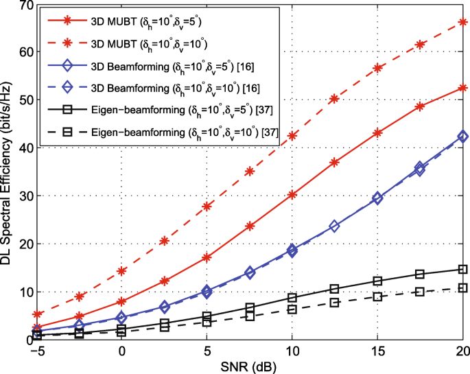
SEs versus average DL receive SNRs in different 3D precoding scenarios

Abbreviations
- 2D:
-
Two-dimensional
- 3D:
-
Three-dimensional
- AS:
-
Angular spread
- BS:
-
Base station
- CCI:
-
Co-channel interference
- CSI:
-
Channel state information
- DoA:
-
Direction of arrival
- DoD:
-
Direction of departure
- DL:
-
Downlink
- FD:
-
Full-duplex
- FDD:
-
Frequency-division duplex
- HD:
-
Half-duplex
- ICI:
-
Inter-cell interference
- IGI:
-
Inter-group interference
- LOS:
-
Light-of-sight
- MIMO:
-
Multiple-input multiple-output
- MMSE:
-
Minimum mean square error
- MUBT:
-
Multiuser beamspace transmission
- MUI:
-
Multiuser interference
- NLOS:
-
Non-ligth-of-sight
- SE:
-
Spectral efficiency
- SI:
-
Self-interference
- SIC:
-
SI cancellation
- SINR:
-
Signal-to-interference-plus-noise ratio
- TDD:
-
Time-division duplex
- UL:
-
Uplink
- ULA:
-
Uniform linear antenna array
- UPA:
-
Uniform planar antenna array
- ZF:
-
Zero-forcing
References
J Mietzner, R Schober, L Lampe, WH Gerstacker, PA Hoeher, Multiple-antenna techniques for wireless communications - a comprehensive literature survey. IEEE Commun. Surv. Tutorials. 11(2), 87–105 (2009).
T Marzetta, Noncooperative cellular wireless with unlimited numbers of base station antennas. IEEE Trans. Wirel. Commun. 9(11), 3590–3600 (2010).
HQ Ngo, E Larsson, T Marzetta, Energy and spectral efficiency of very large multiuser MIMO systems. IEEE Trans. Commun. 61(4), 1436–1449 (2013).
F Fernandes, A Ashikhmin, TL Marzetta, Inter-cell interference in noncooperative TDD large scale antenna systems. IEEE J. Sel. Areas Commun.31(2), 192–201 (2013).
J Hoydis, S Brink, M Debbah, Massive MIMO in UL/DL of cellular networks: how many antennas do we need. IEEE J. Sel. Areas Commun. 31(2), 160–171 (2013).
L You, X Gao, XG Xia, N Ma, Y Peng, Pilot reuse for massive MIMO transmission over spatially correlated rayleigh fading channels. IEEE Trans. Wireless Commun. 14(6), 3352–3366 (2015).
H Cui, L Song, B Jiao, Multi-pair two-way amplify-and-forward relaying with very large number of relay antennas. IEEE Trans. Wireless Commun. 13(5), 2636–2645 (2014).
RCD Lamare, Massive MIMO systems: signal processing challenges and future trends. URSI Radio Science Bulletin. 86(4), 8–20 (2017).
J Jose, A Ashikhmin, TL Marzetta, S Vishwanath, Pilot contamination and precoding in multi-cell TDD systems. IEEE Trans. Wireless Commun. 10(8), 2640–2651 (2011).
N Krishnan, RD Yates, NB Mandayam, Uplink linear receivers for multi-cell multiuser mimo with pilot contamination: large system analysis. IEEE Trans. Wireless Commun. 13(8), 4360–4373 (2014).
A Duly, T Kim, D Love, J Krogmeier, Closed-loop beam alignment for massive MIMO channel estimation. IEEE Commun. Lett. 18(8), 1439–1442 (2014).
A Adhikary, J Nam, J Ahn, G Caire, Joint spatial division and multiplexing-the large-scale array regime. IEEE Trans. Inf. Theory. 59(10), 6441–6463 (2013).
C Sun, X Gao, S Jin, M Matthaiou, Z Ding, C Xiao, Beam division multiple access transmission for massive mimo communications. IEEE Trans. Commun. 63(6), 2170–2184 (2015).
D Ying, FW Vook, TA Thomas, DJ Love, A Ghosh, in IEEE International Conference on Commun. (ICC). Kronecker product correlation model and limited feedback codebook design in a 3D channel model (IEEESydney, 2014), pp. 5865–5870.
Z Wang, W Liu, C Qian, S Chen, L Hanzo, Two-dimensional precoding for 3-d massive mimo. IEEE Trans. Veh. Technol. 66(6), 5485–5490 (2017).
X Li, S Jin, X Gao, RW Heath, Three-dimensional beamforming for large-scale fd-mimo systems exploiting statistical channel state Information. IEEE Trans. Veh. Technol. 65(11), 8992–9005 (2016).
X Li, S Jin, HA Suraweera, J Hou, X Gao, Statistical 3-d beamforming for large-scale mimo downlink systems over rician fading channels. IEEE Trans. Commun. 64(4), 1529–1543 (2016).
Z Zhang, X Chai, K Long, AV Vasilakos, L Hanzo, Full duplex techniques for 5G networks: self-interference cancellation, protocol design, and relay selection. IEEE Commun. Mag. 53(5), 128–137 (2015).
D Kim, H Lee, D Hong, A survey of in-band full-duplex transmission: from the perspective of PHY and MAC layers. IEEE Commun. Surv. Tutorials. 17(4), 2017–2046 (2015).
A Sabharwal, P Schniter, D Guo, DW Bliss, S Rangarajan, R Wichman, In-band full-duplex wireless: challenges and opportunities. IEEE J. Sel. Areas Commun. 32(9), 1637–1652 (2014).
C Psomas, M Mohammadi, I Krikidis, HA Suraweera, Impact of directionality on interference mitigation in full-duplex cellular networks. IEEE Trans. Wireless Commun. 16(1), 487–502 (2017).
M Mohammadi, HA Suraweera, Y Cao, I Krikidis, C Tellambura, Full-duplex radio for uplink/downlink wireless access with spatially random nodes. IEEE Trans. Commun. 63(12), 5250–5266 (2015).
J Lee, TQS Quek, Hybrid full-/half-duplex system analysis in heterogeneous wireless networks. IEEE Trans. Wirel. Commun. 14(5), 2883–2895 (2015).
HQ Ngo, HA Suraweera, M Matthaiou, EG Larsson, Multipair full-duplex relaying with massive arrays and linear processing. IEEE J. Sel. Areas Commun. 32(9), 1721–1737 (2014).
X Xia, D Zhang, K Xu, W Ma, Y Xu, Hardware Impairments Aware Transceiver for Full-Duplex Massive MIMO Relaying. IEEE Trans. Signal Process. 63(24), 6565–6580 (2015).
M Mohammadi, BK Chalise, HA Suraweera, Z Ding, in IEEE International Conference on Communications. Wireless information and power transfer in full-duplex systems with massive antenna arrays (IEEEParis, 2017), pp. 1–6.
Y Li, P Fan, A Leukhin, L Liu, On the Spectral and energy efficiency of full-duplex small-cell wireless systems with massive mimo. IEEE Trans. Veh. Technol. 66(3), 2339–2353 (2017).
X Xia, Y Xu, K Xu, D Zhang, W Ma, Full-duplex massive mimo AF relaying with semiblind gain control. IEEE Trans. Veh. Technol. 65(7), 5797–5804 (2016).
H Yin, D Gesbert, M Filippou, Y Liu, A coordinated approach to channel estimation in large-scale multiple-antenna systems. IEEE J. Sel. Areas Commun. 31(2), 264–273 (2013).
JP Kermoal, L Schumacher, KI Pedersen, PE Mogensen, F Frederiksen, A stochastic MIMO radio channel model with experimental validation. IEEE J. Sel. Areas Commun. 20(6), 1211–1226 (2002).
B Clerckx, C Oestges, MIMO Wireless Networks: Channels, Techniques and Standards for Multi-Antenna, Multi-User and Multi-Cell Systems. 2nd (Academic Press, Oxford, 2013).
J Wang, R Zhang, W Duan, SX Lu, L Cai, in Proc. ICC 2014. Angular spread measurement and modeling for 3D MIMO in urban macrocellular radio channels (IEEESydney, 2014), pp. 20–25.
MA Maddah-Ali, DNC Tse, Completely stale transmitter channel state information is still very useful. IEEE Trans. Inform. Theory. 58(7), 4418–4432 (2012).
T Kailath, AH Sayed, B Hassibi, Linear Estimation (Upper Saddle River, Prentice-Hall, 2000).
B Hassibi, BM Hochwald, How much training is needed in multiple-antenna wireless links?IEEE Trans. Inf. Theory. 49(4), 951–963 (2003).
3GPP TR 36.828, Further enhancements to LTE time division duplex (TDD) for downlink-uplink (DL-UL) interference management and traffic adaptation. (2012). v.11.0.0. www.3gpp.org. Accessed 7 Aug 2018.
Y Song, S Nagata, H Jiang, L Chen, in IEEE International Conference on Communications. CSI-RS design for 3D MIMO in future LTE-Advanced (IEEESydney, 2014), pp. 5101–5106.
G Caire, N Jindal, M Kobayashi, N Ravindran, Multiuser MIMO achievable rates with downlink training and channel state feedback. IEEE Trans. Inf. Theory. 56(6), 2845–2866 (2010).
J Choi, D Love, T Kim, Trellis-extended codebooks and successive phase adjustment: A path from LTE-Advanced to FDD massive MIMO systems. IEEE Trans. Wirel. Commun. 14(4), 2007–2016 (2015).
Funding
This research was supported by the National Natural Science Foundation of China (No. 61671472), Jiangsu Province Natural Science Foundation (BK20160079), and National Natural Science Foundation of China (No. 61371123, No. 91438115).
Author information
Authors and Affiliations
Contributions
XW is the main writer of this paper. He proposed the main idea, conducted the simulations, and analyzed it. DZ, KX, and WM assisted the review of this manuscript. All authors read and approved the final manuscript.
Corresponding author
Ethics declarations
Competing interests
The authors declare that they have no competing interests.
Publisher’s Note
Springer Nature remains neutral with regard to jurisdictional claims in published maps and institutional affiliations.
Rights and permissions
Open Access This article is distributed under the terms of the Creative Commons Attribution 4.0 International License (http://creativecommons.org/licenses/by/4.0/), which permits unrestricted use, distribution, and reproduction in any medium, provided you give appropriate credit to the original author(s) and the source, provide a link to the Creative Commons license, and indicate if changes were made.
About this article

Cite this article
Zhang, D., Wang, X., Xu, K. et al. Multiuser 3D massive MIMO transmission in full-duplex cellular system. J Wireless Com Network 2018, 203 (2018). https://doi.org/10.1186/s13638-018-1219-x
Received:
Accepted:
Published:
DOI: https://doi.org/10.1186/s13638-018-1219-x