- Research
- Open access
- Published:
Cognitive decode-and-forward relaying with successive interference cancelation
EURASIP Journal on Wireless Communications and Networking volume 2018, Article number: 234 (2018)
Abstract
In this work, we study the cognitive decode-and-forward (DF) relaying, where a primary user (PU) communicates with an access point (AP), and in the same geographical region, a secondary source (SS) communicates to a secondary destination (SD) with assistance from a secondary relay (SR). Either SR or SD can decode the secondary data directly (DIR) or using the successive interference cancelation (SIC) technique. Based on the decoding methods of SR and SD, we proposed SR-DIR-SD-DIR, SR-DIR-SD-SIC, SR-SIC-SD-DIR, and SR-SIC-SD-SIC-based cognitive DF relaying schemes. The outage probabilities of both primary and secondary systems are analyzed for all the decoding manners. The transmit powers of SS and SR are further determined to minimize the outage probability of secondary system subject to the constraint that the outage performance loss of primary system should not exceed a certain percentage compared with the stand-alone primary network without spectrum sharing. Numerical results show that by using the SIC decoding, the outage probability of secondary system can be greatly decreased, especially when the interference from PU is strong or the transmission rate of primary data is low.
1 Introduction
Spectrum sharing schemes have been extensively studied to meet the ever-growing wireless transmission requirements using the licensed spectrum, which is often under-utilized across time and space. Primary users (PUs) own the licensed spectrum and have higher priorities of accessing it. Secondary users (SUs) can share the spectrum under the performance constraint of primary system [1]. Traditionally, SUs could sense the spectrum to see whether it is used by PUs or not and opportunistically access the idle spectrum. If the spectrum is busy for a long time, SUs can rarely access it [2]. Instead, SUs can transmit concurrently with PUs, but they should carefully control their powers to avoid violating the performance constraint of primary system [3]. Furthermore, SUs can cooperatively transmit primary data to exchange some resources for the spectrum access [4]. In the multiple SU scenario, the primary data can be quickly delivered with assistance from a selected SU, so the secondary data can be transmitted in the remaining time over the spectrum [5]. SU can also help exchange primary data in the two-way system and superposes the secondary transmission on network-coded primary signals [6, 7].
1.1 Related works
For the underlay spectrum sharing, the concurrent transmissions of PUs and SUs will cause mutual interferences between them. In order to guarantee the interference constraint of primary system, the transmit powers of SUs should be conservatively set, especially when they are close to PUs, so the transmission requirements of SUs can be hardly satisfied [8, 9]. It becomes more difficult to satisfy the quality of service (QoS) requirements of multiple SUs under the interference temperature constraint [10]. By introducing a secondary relay (SR) between a secondary source (SS) and a secondary destination (SD), the distance of each hop can be shortened and the communication reliability can be enhanced [11–14]. Both SS and SR should strictly control their transmit powers to avoid causing intolerable interference to the primary system, so the cooperative diversity is lost [15, 16]. Either the interference-alignment or the beamforming technique can be adopted by PUs and SUs to mitigate the mutual interference [17, 18]. An adaptive power allocation scheme was proposed in [19], where SUs can access the power control signaling of PUs and control their powers in both the long-time and short-time scales to improve the capacity of secondary system while guaranteeing the QoS of PUs [19]. Since the underlay mode will result in low transmission efficiency due to restricted power, to maximize the throughput of secondary system, researchers have proposed dynamic overlay-underlay and interweave-underlay spectrum sharing schemes based on the statuses of PUs [20–23].
In the underlay spectrum sharing, SUs can implicitly access the spectrum without coordinating with PUs, and it is useful when the distances between SUs and PUs are long, as higher powers can be allowable for the secondary data transmission. For the cognitive relaying, SS and SD could exchange information via SR using network coding to improve the spectral efficiency [24–26] or selecting a best relay for the two-way relaying [27]. For the full-duplex relaying, SR will suffer the interference from not only PUs but also itself, and higher spectral efficiency can be achieved compared with the half-duplex mode [28]. If PUs transmit with the in-band full-duplex mode, the self-interference in the primary system will impede the opportunity of spectrum access for SUs [29]. For the multiuser cognitive relaying, a SU could select the best relay and destination to cooperatively transmit data by properly adjusting their powers [30–33]. If the SUs can harvest energy from the primary data transmission, then they can use the harvest energy to cooperatively forward the primary data and meanwhile transmit the secondary data using the Alamouti coding [34].
In large-scale cognitive radio networks, PUs and SUs are randomly distributed on the plane, and their locations can be modeled as an independent homogeneous Poisson point process (PPP). The interference encountered at a typical receiver comes from all the active PUs and SUs on the plane except the dedicated transmitter. It is vitally important to properly model the aggregated interference at a typical receiver for the performance analysis. The transmission capacity was analyzed for a cognitive ad hoc network underlaying cellular network [35, 36]. If SUs could access the spectrum only when they lie outside the exclusive regions of PUs, the active SUs can be modeled as a Poisson hole process and the performance was analyzed by approximating their distribution as a PPP [37, 38]. Zhai et al. applied a cooperation zone between each base station (BS) and cell-edge users, wherein a SU is selected to cooperatively forward the primary data to exchange for some disjoint bandwidth for the secondary data transmission [39]. In cellular networks, device-to-device (D2D) communications can greatly reduce the transmit powers of users, and D2D users can share the spectrum of cellular users to improve the spectral efficiency [40–42]. If PUs are capable of harvesting wireless energy to sustain their operations, the best SU in the energy cooperation zone can be selected to wirelessly charge PUs to exchange for some disjoint bandwidths for the secondary data transmission [43], or SUs can opportunistically transmit secondary data only when they lie outside the guard zones of PUs [44].
1.2 Motivation and contribution
In the traditional cognitive relaying scheme, both SR and SD decode the secondary data directly by treating the received primary signal as interference. The cognitive relaying scheme works properly only when the mutual interferences between PUs and SUs are weak enough. For the successful operation of traditional cognitive relaying, the distances between SUs and PUs should be long enough, so the mutual interference is greatly weakened due to the strong path-loss. When the distances between SUs and PUs are moderate or short, to avoid violating the interference constraint of primary system, the transmit powers of SS and SR are often set very small. Meanwhile, SR and SD could encounter very strong interference from PUs. Due to the weak signal and the strong interference, the communication performance of secondary system is very bad. Inspired by this fact, we proposed the interference cancelation-based cognitive relaying scheme to improve the spectral efficiency.
In this work, we consider a general scenario, where SUs may be close to PUs or far away. We propose to enable either SR or SD or both of them to decode secondary data using the successive interference cancelation (SIC) technique. Considering SR or SD performs the direct (DIR) decoding or the SIC decoding, we proposed cognitive relaying schemes with SR-DIR-SD-DIR, SR-DIR-SD-SIC, SR-SIC-SD-DIR, and SR-SIC-SD-SIC decoding manners. The outage probabilities of both primary and secondary systems are analyzed. Under the constraint that the outage performance loss of primary system should not exceed a certain ratio compared with the none sharing scenario, the transmit powers of SS and SR are determined by minimizing the outage probability of secondary system. Numerical results show that the outage performance of secondary system can be significantly improved by using the SIC technique, as the strong interference from PUs can be effectively suppressed, and the total network throughput can be greatly boosted compared with the none spectrum sharing scenario. With smaller transmission rate of primary data, SR and SD could correctly decode and cancel the primary data more easily, so the outage performance of secondary system gets better. If more performance loss can be tolerated by the primary system, a lower outage probability can be achieved for the secondary system, as higher powers can be used by SS and SR for the secondary data transmission.
The rest of this paper is organized as follows. Section 2 briefly outlines the methods. Section 3 illustrates our proposed cognitive relaying scheme with SIC. Sections 4 and 5 analyze the outage probability of primary system and secondary system, respectively. The transmit powers of SS and SR are determined in Section 6. Results and discussion are presented in Section 7. Finally, Section 8 concludes this paper.
2 Methods
We consider a cognitive decode-and-forward (DF) relaying system as shown in Fig. 1, where PU communicates to an access point (AP), and meanwhile, SS communicates to SD with assistance from SR. Each node has one omnidirectional antenna and works in the half-duplex mode. The transmission time is divided into equal-length blocks, and each block is normalized to have 1 s. The Rayleigh block fading is assumed for each channel, which keeps invariant in each block, but changes independently across different links and blocks. Due to the blockage or deep fading, we assume that there is no direct link between SS and SD, so the data transmission from SS to SD should be forwarded by SR. The DF protocol is adopted by SR for the secondary data relaying. We assume that SR and SD know the related channel state information (CSI) in each block, so they can perform the DIR decoding or the SIC decoding. For the DIR decoding, after receiving the composite signals from SS and PU, SR and SD directly decode the secondary data by treating the received primary signal as interference. For the SIC decoding, SR and SD could decode the primary data and then cancel it from the received composite signal, and after that, they will try to decode the secondary data without interference.

Cognitive DF relaying with SIC decoding at SR and SD
We assume that both PU and SS do not know the instantaneous CSI towards their intended receivers; thus, they transmit their data with fixed rates. The transmission rates of primary data and secondary data are denoted as Rp and Rs, respectively. The data transmission is assumed to be successful if the channel achievable rate is greater than the transmission rate. The channel achievable rates of primary system and secondary system are denoted as Cp= log2(1+γ) and \(C_{\mathrm {s}}=\frac {1}{2}\log _{2}\left (1+\gamma \right)\), respectively, where γ denotes the signal-to-noise-ratio (SNR) or signal-to-interference-plus-noise-ratio (SINR) of the received signal. Through the expressions of Cp≥Rp and Cs≥Rs, we can equivalently obtain the SNR or SINR thresholds as \(\phantom {\dot {i}\!}\xi _{\mathrm {p}}=2^{R_{\mathrm {p}}}-1\) and \(\phantom {\dot {i}\!}\xi _{\mathrm {s}}=2^{2R_{\mathrm {s}}}-1\), respectively. Therefore, the primary data and secondary data are assumed to be successfully decoded if the received SNR and SINR are greater than ξp and ξs, respectively; otherwise, the outage event occurs. We analyze the outage probabilities of both primary and secondary systems by considering the DIR or the SIC decoding at SR and SD. Expectations are taken over power fadings of different channels, which are independently and exponentially distributed with unit mean.
We aim to minimize the outage probability of the secondary system while satisfying that the outage performance loss of the primary system should not exceed ε percentage compared with the none spectrum sharing scenario. The optimal transmit powers of SS and SR are jointly determined through minimizing the outage probability of the secondary system while guaranteeing the performance constraint of primary system. Numerical and simulation results are provided to validate our theoretical analysis and verify that our proposed scheme can greatly improve the outage performance of secondary system.
3 Cognitive relaying with DIR and SIC decoding
3.1 Cognitive relaying process
The transmission process is shown in Fig. 2. In each block, PU always transmits a new primary data packet to AP. In an even block 2n, (n=0,1,...), SS transmits a secondary data packet to SR. If SR correctly decodes the secondary data from SS, it will forward the secondary data to SD in the odd block 2n+1; otherwise, if SR erroneously decodes the secondary data, it will keep silent in the odd block 2n+1. The secondary data receptions at SR and SD are interfered by the primary data transmission of PU. The primary data reception at AP is interfered by the secondary data transmissions of SS and SR. AP decodes the primary data directly by treating the received secondary data as interference, while SR and SD decode the secondary data using the DIR or the SIC scheme:
-
SR-DIR-SD-DIR: Both SR and SD decode the secondary data directly by treating the received primary data as interference.
Fig. 2 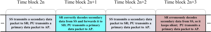
Transmission process of the cognitive DF relaying with n=0,1,...
-
SR-DIR-SD-SIC: Both SR and SD perform the DIR decoding. If SD erroneously decodes the secondary data, it will try to decode and cancel the primary data to further decode the secondary data.
-
SR-SIC-SD-DIR: Both SR and SD perform the DIR decoding. If SR erroneously decodes the secondary data, it will try to decode and cancel the primary data to further decode the secondary data.
-
SR-SIC-SD-SIC: Both SR and SD perform the DIR decoding. If SR or SD erroneously decodes the secondary data, it will try to decode and cancel the primary data to further decode the secondary data.

Remark: SR and SD try to decode the secondary data directly, and if not successful, the SIC decoding may be performed. Intuitively, the stronger the interference from PU, the more difficult for SR and SD to decode the secondary data directly, but the more easily for them to decode and cancel the interference. If the two systems are close, the interference is strong, so the SIC decoding performs better than the DIR decoding. If the two systems are departed far away, the interference is weak, so the SIC decoding achieves a similar performance as the DIR decoding. The SIC decoding always outperforms the DIR decoding, but the cost is that SR or SD should know the CSI and codebook of PU for the interference cancelation. To avoid the security issue, we assume that PU firstly encrypts the primary information and then transmits it by appending the error detection code, such as the cyclic redundancy check (CRC) code. SR and SD can decode the primary data without endangering the security of primary information.
3.2 SINR and SNR at AP
In an even block, when SS transmits secondary data to SR along with PU transmitting primary data to AP, with the interference from SS, the SINR of primary data reception at AP is denoted as γpsa and given by
where pp and ps represent the transmit power of PU and SS, respectively; Gpa and Gsa represent the small-scale power fading of the channel PU →AP and SS →AP, respectively; ℓpa and ℓsa represent the large-scale path-loss of the channel PU →AP and SS →AP, respectively; and N0 is the power of additive white Gaussian noise (AWGN) at each receiver.
In an odd block, when SR forwards secondary data to SD along with PU transmitting primary data to AP, with the interference from SR, the SINR of primary data reception at AP is denoted as γpra and given by
where pr is the transmit power SR; Gra and ℓra represent the small-scale power fading and the large-scale path-loss of the channel SR →AP, respectively.
For the stand-alone primary network without spectrum sharing from SUs, the data reception at AP is interference-free. For the cognitive DF relaying, if SR erroneously decodes the secondary data in an even block, it will keep silent in the next odd block and the primary data reception at AP is also interference-free. If there is no interference, the SNR of the primary data reception at AP is denoted as γpa and given by
So far, we have presented the SINR and SNR of the received primary signal at AP, which will be used later for the outage performance analysis.
3.3 SINR and SNR at SR
In an even block, when SS transmits secondary data along with PU transmitting primary data to AP, with the interference from PU, the SINR of the secondary data reception at SR is denoted as γspr and given by
where Gsr and Gpr represent the small-scale power fading of the channel SS →SR and PU →SR, respectively, and ℓsr and ℓpr represent the large-scale path-loss of the channel SS →SR and PU →SR, respectively.
For the SIC decoding, if the direct decoding of secondary data fails at SR, it will try to decode and cancel the primary data to further decode the secondary data. By viewing the secondary data as interference, the SINR of primary data reception at SR is denoted as γpsr and given by
If the primary data can be successfully decoded and canceled by SR, the SNR of the remaining secondary data is denoted as γsr and given by
So far, we have presented the SINR and SNR of the received signals at SR, which will be used later to analyze the probability of SR correctly decoding the secondary data.
3.4 SINR and SNR at SD
In an odd block, when SR forwards secondary data along with PU transmitting primary data to AP, with the interference from PU, the SINR of secondary data reception at SD is denoted as γrpd and given by
where Grd and Gpd represent the small-scale power fading of the channel SR →SD and PU →SD, respectively, and ℓrd and ℓpd represent the large-scale path-loss of the channel SR →SD and PU →SD, respectively.
If SD can perform the SIC, it will first try to decode the secondary data directly. If the direct decoding of secondary data fails, SD will try to decode and cancel the primary data. By viewing the secondary data as interference, the SINR of primary data reception at SD is denoted as γprd and given by
If the primary data can be successfully decoded and canceled by SD, the SNR of the remaining secondary data is denoted as γrd and given by
So far, we have presented the SINR and SNR of the received signals at SD, which will be used later for the outage performance analysis.
4 Outage probability of primary system
4.1 Stand-alone primary system
For the stand-alone primary network without spectrum sharing from SUs, the SNR of received primary data at AP is γpa given in (3). Denoted as \(P_{\text {outp}}^{\text {NS}}\), the outage probability of primary data transmission in the none spectrum sharing scenario is \(P_{\text {outp}}^{\text {NS}}=\Pr \left \{\gamma _{\text {pa}}<\xi _{\mathrm {p}}\right \}\), obtained as
where we consider that the power fading Gpa is exponentially distributed with unit mean.
4.2 Cognitive DF relaying
For the cognitive DF relaying, the outage probability of primary system is denoted as Poutp. Let \(\mathcal {A}\) denote the event that SR correctly decodes the secondary data from SS in an even block. When the event \(\mathcal {A}\) occurs, SR will forward the secondary data to SD in the next odd block. With the interference from SS and SR, the average outage probability of primary system is given as
where \(\mathcal {\bar {A}}\) denotes the complement event of \(\mathcal {A}\). The first term represents the outage probability of primary data decoding in even blocks with interference from SS. The second and third terms represent the outage probabilities of primary data decoding in odd blocks when SR forwards the secondary data or keeps silent in case \(\mathcal {A}\) or \(\mathcal {\bar {A}}\) occurs. The prefactor 1/2 is used, as we consider the primary data transmission in both the even and odd blocks. Next, we will analyze the three terms of (11) by considering whether the DIR or the SIC decoding is performed by SR.
4.2.1 First term of (11)
By substituting the expression of γpsa, we can derive
where we consider that Gpa and Gsa are independently and exponentially distributed with unit mean. With the increase of ps, SS causes more interference to AP in even blocks, so the outage probability Pr{γpsa<ξp} gets larger.
4.2.2 Second term of (11) with SR-DIR
If SR performs the DIR decoding, we can express the second term of (11) as \(\Pr \left \{\mathcal {A},\gamma _{\text {pra}}<\xi _{\mathrm {p}}\right \}=\Pr \left \{\gamma _{\text {spr}}\ge \xi _{\mathrm {s}}, \gamma _{\text {pra}}<\xi _{\mathrm {p}}\right \}\), derived as
where we consider that Gsr, Gpr, Gpa, and Gra are all independently and exponentially distributed with unit mean. With the increase of ps, SR could decode the secondary data more easily and then transmits in odd blocks, which causes more interference to AP and leads to a larger outage probability of \(\Pr \left \{\mathcal {A},\gamma _{\text {pra}}<\xi _{\mathrm {p}}\right \}\).
4.2.3 Second term of (11) with SR-SIC
If SR performs the SIC decoding, by considering the cases of SR correctly decoding the secondary data, we can express the second term of (11) as
where the first probability considers that SR correctly decodes the secondary data directly; the second probability considers that SR fails in decoding the secondary data directly, but it correctly decodes the secondary data after successfully decoding and canceling the primary data. The first probability of (14) has been derived in (13) and the second probability can be derived as
where \(\mathbf {1}(\mathcal {C})\) is an indicator random variable, which equals one if the condition \(\mathcal {C}\) is satisfied; otherwise, it equals zero, and
The derivation details of (15) are given in Appendix 1.
Substituting (13) and (15) into (14), we can obtain the second probability of (11) when SR performs the SIC decoding.
4.2.4 Third term of (11) with SR-DIR
If SR performs the DIR decoding, we can express the third term of (11) as \(\Pr \left \{\mathcal {\bar {A}},\gamma _{\text {pa}}<\xi _{\mathrm {p}}\right \}=\Pr \left \{\gamma _{\text {spr}}<\xi _{\mathrm {s}},\gamma _{\text {pa}}<\xi _{\mathrm {p}}\right \}\), derived as
With the increase of ps, \(\mathcal {\bar {A}}\) occurs less likely, so SR will cause less interference to AP in odd blocks, resulting in the lower outage probability of \(\Pr \left \{\mathcal {\bar {A}},\gamma _{\text {pa}}<\xi _{\mathrm {p}}\right \}\).
4.2.5 Third term of (11) with SR-SIC
If SR performs the SIC decoding, by considering the cases of SR erroneously decoding the secondary data, we can express the third term of (11) as
where the first probability considers that both the direct decoding of secondary data and the cancelation of primary data are not successful at SR; the second probability considers that SR fails in decoding the secondary data directly, even after successfully canceling the primary data. The first term of (18) is derived as
where
The derivation details of (19) are given in Appendix 2.
The second term of (18) can be derived as
Substituting (19) and (21) into (18), we can obtain the third probability of (11) when SR performs the SIC decoding.
5 Outage probability of secondary system
5.1 SR-DIR-SD-DIR decoding
In the SR-DIR-SD-DIR scheme, both SR and SD decode secondary data directly by treating the received primary data as interference. For this scheme, the outage probability of secondary system is given as
where \(P_{\text {outs}}^{\mathrm {SR-DIR}}\) and \(P_{\text {outs}}^{\mathrm {SD-DIR}}\) represent the outage probability of DIR decoding of secondary data at SR and SD, respectively. The first term represents the probability of SR erroneously decoding the secondary data directly. The second term represents the probability that SR correctly decodes the secondary data but SD erroneously decodes the secondary data forwarded by SR. Since the channel SS →SR is independent with the channel SR →SD, we can write the second term as the multiplication of two probabilities.
The outage probability of SR directly decoding secondary data can be expressed as \(P_{\text {outs}}^{\mathrm { SR-DIR}}=\Pr \left \{\gamma _{\text {spr}}<\xi _{\mathrm {s}}\right \}\), derived as
where we consider that Gsr and Gpr are independently and exponentially distributed with unit mean.
If SR correctly decodes the secondary data from SS in the even block, it will forward the secondary data to SD in the next odd block. The probability of SD erroneously decoding the secondary data directly is \(P_{\text {outs}}^{\mathrm { SD-DIR}}=\Pr \left \{\gamma _{\text {rpd}}<\xi _{\mathrm {s}}\right \}\), i.e.,
where we consider that Grd and Gpd are independently and exponentially distributed with unit mean.
5.2 SR-DIR-SD-SIC decoding
In the SR-DIR-SD-SIC scheme, SR and SD perform DIR and SIC decoding, respectively. If SD fails in decoding the secondary data directly, it will try to decode and cancel the primary data for the further decoding of secondary data. For this scheme, the outage probability of secondary system is given as
where \(P_{\text {outs}}^{\mathrm {SD-SIC}}\) represents the outage probability of SIC decoding at SD.
The outage probability of direct decoding at SR that is \(P_{\text {outs}}^{\mathrm {SR-DIR}}\) has been derived in (23). The outage probability of SIC decoding at SD can be expressed as
where the first probability represents that both the direct decoding of secondary data and the cancelation of primary data are not successful at SD; the second probability represents that SD fails in decoding the secondary data, even after successfully canceling the primary data.
By substituting the related items into (26), we can derive the first probability as
-
If ξpξs>1, we have
$$\begin{array}{*{20}l} P_{\mathrm{outs1}}^{\mathrm{SD-SIC}}=&1-\frac{p_{\mathrm{p}}\ell_{\text{pd}}}{p_{\mathrm{p}}\ell_{\text{pd}}+\xi_{\mathrm{p}}p_{\mathrm{ r}}\ell_{\text{rd}}}\exp\left(-\frac{\xi_{\mathrm{p}}N_{0}}{p_{\mathrm{p}}\ell_{\text{pd}}}\right)\\ &-\frac{p_{\mathrm{r}}\ell_{\text{rd}}}{p_{\mathrm{r}}\ell_{\text{rd}}+\xi_{\mathrm{s}}p_{\mathrm{p}}\ell_{\mathrm{ pd}}}\exp\left(-\frac{\xi_{\mathrm{s}}N_{0}}{p_{\mathrm{r}}\ell_{\text{rd}}}\right). \end{array} $$(27) -
If ξpξs≤1, we have
$$ {\begin{aligned} P_{\mathrm{outs1}}^{\mathrm{SD-SIC}}=&1-\exp\left(-\frac{\xi_{\mathrm{p}}N_{0}}{p_{\mathrm{p}}\ell_{\text{pd}}}\right)-\frac{p_{\mathrm{ r}}\ell_{\text{rd}}}{p_{\mathrm{r}}\ell_{\text{rd}}+\xi_{\mathrm{s}}p_{\mathrm{p}}\ell_{\text{pd}}}\exp\left(-\frac{\xi_{\mathrm{ s}}N_{0}}{p_{\mathrm{r}}\ell_{\text{rd}}}\right)\\ &\times\left\{1-\exp\left[-\left(1+\frac{\xi_{\mathrm{s}}p_{\mathrm{p}}\ell_{\text{pd}}}{p_{\mathrm{r}}\ell_{\mathrm{ rd}}}\right)\frac{(1+\xi_{\mathrm{s}})\xi_{\mathrm{p}}N_{0}}{(1-\xi_{\mathrm{p}}\xi_{\mathrm{s}})p_{\mathrm{p}}\ell_{\mathrm{ pd}}}\right]\right\}\\ &+\frac{\xi_{\mathrm{p}}p_{\mathrm{r}}\ell_{\text{rd}}}{p_{\mathrm{p}}\ell_{\text{pd}}+\xi_{\mathrm{p}}p_{\mathrm{r}}\ell_{\mathrm{ rd}}}\left\{\exp\left(-\frac{\xi_{\mathrm{p}}N_{0}}{p_{\mathrm{p}}\ell_{\text{pd}}}\right)\right.\\ &\left.-\exp\left[-\left(1+\frac{p_{\mathrm{p}}\ell_{\text{pd}}}{\xi_{\mathrm{p}}p_{\mathrm{r}}\ell_{\mathrm{ rd}}}\right)\frac{(1+\xi_{\mathrm{s}})\xi_{\mathrm{p}}N_{0}}{(1-\xi_{\mathrm{p}}\xi_{\mathrm{s}})p_{\mathrm{p}}\ell_{\mathrm{ pd}}}+\frac{N_{0}}{p_{\mathrm{r}}\ell_{\text{rd}}}\right]\right\}. \end{aligned}} $$(28)
The second probability of (26) can be expressed as \(P_{\mathrm {outs2}}^{\mathrm {SD-SIC}}=\Pr \left \{\gamma _{\text {prd}}\ge \xi _{\mathrm {p}},\gamma _{\text {rd}}<\xi _{\mathrm { s}}\right \}\) and derived as
Substituting (27), (28), and (29) into (26), we can obtain the outage probability of SD performing the SIC decoding of secondary data.
5.3 SR-SIC-SD-DIR decoding
In the SR-SIC-SD-DIR scheme, SR and SD perform SIC and DIR decoding, respectively. If SR fails in decoding the secondary data directly, it will try to decode and cancel the primary data to further decode the secondary data. For this scheme, the outage probability of secondary system is given as
where \(P_{\text {outs}}^{\mathrm {SR-SIC}}\) represents the outage probability of SIC decoding at SR. The probability \(P_{\text {outs}}^{\mathrm {SR-SIC}}\) can be derived similarly as (26) by replacing pr, dpd, and drd with ps, dpr, and dsr, respectively. The outage probability of DIR decoding at SD that is \(P_{\text {outs}}^{\mathrm {SD-DIR}}\) has been derived in (24).
5.4 SR-SIC-SD-SIC decoding
In the SR-SIC-SD-SIC scheme, both SR and SD perform the SIC decoding. If SR or SD fails in decoding the secondary data directly, they will try to decode and cancel the primary data to further decode the secondary data. In this scheme, the outage probability of secondary system is given as
The outage probability \(P_{\text {outs}}^{\mathrm {SR-SIC}}\) can be derived similarly as (26) by replacing pr, dpd, and drd with ps, dpr, and dsr, respectively. The outage probability of SIC decoding at SD that is \(P_{\text {outs}}^{\mathrm {SD-SIC}}\) has been derived in (26).
6 Power settings for SS and SR
Compared with the stand-alone primary network without spectrum sharing, the outage probability of primary system in the cognitive relaying can be degraded no more than ε percentage. The optimization problem can be formulated as
For the secondary system, Pouts can be (22), (25), (30), or (31) for the DIR or the SIC decoding at SR and SD. For the primary system, Poutp is obtained in (11) by considering the DIR or the SIC decoding at SR. The transmit powers of SS and SR can not exceed pm due to the hardware or regulation constraint. Since the maximal value of Poutp is smaller than 1, we have to constrain \((1+\epsilon)P_{\text {outp}}^{\text {NS}}\le 1\), that is \(\epsilon \le \frac {1}{P_{\text {outp}}^{\text {NS}}}-1\), where \(P_{\text {outp}}^{\text {NS}}\) is derived in (10).
6.1 Impacts and region of p s
If we set pr=0, only SS transmits secondary data in even blocks, and there is no secondary data transmission in odd blocks. For a given value of ps, we can derive a lower bound of the outage probability of primary system, i.e.,
where the first probability is obtained in (12) and the secondary probability is \(P_{\mathrm { outp}}^{\text {NS}}\) given in (10). Since \(\check P_{\text {outp}}\) is a monotonically increasing function of ps, we can determine an allowable region of ps as follows:
-
Case I: Let ps=pm, if \(\check P_{\text {outp}}\ge (1+\epsilon)P_{\text {outp}}^{\text {NS}}\), calculate \(p_{\mathrm {s}}^{\dagger }\) via \(\check P_{\text {outp}}=(1+\epsilon)P_{\text {outp}}^{\text {NS}}\) that is \(\Pr \left \{\gamma _{\text {psa}}<\xi _{\mathrm {p}}\right \}=(1+2\epsilon)P_{\text {outp}}^{\text {NS}}\). To make the equation meaningful, we set \((1+2\epsilon)P_{\text {outp}}^{\text {NS}}\le 1\) that is \(\epsilon \le \frac {1}{2}\left (\frac {1}{P_{\text {outp}}^{\text {NS}}}-1\right)\). An upper bound of the transmit power of SS can be derived as
$$\begin{array}{*{20}l} p_{\mathrm{s}}^{\dagger}=\frac{p_{\mathrm{p}}\ell_{\text{pa}}}{\xi_{\mathrm{p}}\ell_{\text{sa}}}\left[ \frac{\exp\left(-\frac{\xi_{\mathrm{p}}N_{0}}{p_{\mathrm{p}}\ell_{\text{pa}}}\right)}{1-(1+2\epsilon)P_{\text{outp}}^{\mathrm{ NS}}}-1\right]. \end{array} $$(34) -
Case II: Let ps=pm, if \(\check P_{\text {outp}}< (1+\epsilon)P_{\text {outp}}^{\text {NS}}\), the critical power is set as \(p_{\mathrm {s}}^{\dagger }=p_{\mathrm {m}}\).
Thus, the transmit power of SS should be constrained in the region of \(p_{\mathrm {s}}\in \left [0,p_{\mathrm { s}}^{\dagger }\right ]\).
6.2 Impacts and region of p r
As can be seen from (11), no matter whether SR performs the DIR or the SIC decoding, Poutp always increases monotonically with pr. Given ps, we should determine a critical power of SR, denoted as \(p_{\mathrm {r}}^{\dagger }(p_{\mathrm {s}})\). This critical value means that if the transmit power of SR is smaller than \(p_{\mathrm {r}}^{\dagger }(p_{\mathrm {s}})\), the outage performance constraint of primary system can be guaranteed; otherwise, it is violated.
-
Case I: Let pr=pm, if \(P_{\text {outp}}\ge (1+\epsilon)P_{\text {outp}}^{\text {NS}}\), then do the following calculation: Let pr=0, if \(P_{\text {outp}}<(1+\epsilon)P_{\text {outp}}^{\text {NS}}\), calculate \(p_{\mathrm {r}}^{\dagger }(p_{\mathrm {s}})\) via \(P_{\text {outp}}=(1+\epsilon)P_{\text {outp}}^{\text {NS}}\); otherwise, if \(P_{\text {outp}}\ge (1+\epsilon)P_{\text {outp}}^{\text {NS}}\), the given ps is not valid.
-
Case II: Let pr=pm, if \(P_{\text {outp}}< (1+\epsilon)P_{\text {outp}}^{\text {NS}}\), the critical power is \(p_{\mathrm {r}}^{\dagger }(p_{\mathrm {s}})=p_{\mathrm {m}}\).
Considering whether SR performs the DIR or the SIC decoding, the critical power \(p_{\mathrm {r}}^{\dagger }(p_{\mathrm {s}})\) in case I can be determined as follows.
6.2.1 SR-DIR decoding
If SR performs the DIR decoding, the critical power is obtained as
where
with \(P_{\text {outp}}^{\text {NS}}\), Pr{γpsa<ξp}, and \(\Pr \left \{\mathcal {\bar A},\gamma _{\text {pa}}<\xi _{\mathrm {p}}\right \}\) given in (10), (12), and (17), respectively.
6.2.2 SR-SIC decoding
If SR performs the SIC decoding, the critical power is obtained as
where
with ftem1 given in (16) and \(\Pr \left \{\mathcal {\bar {A}},\gamma _{\text {pa}}<\xi _{\mathrm {p}}\right \}\) given in (18).
6.3 Transmit powers of SS and SR
The transmit power of SS can be numerically searched in the region of \(p_{\mathrm {s}}\in \left [0,p_{\mathrm {s}}^{\dagger }\right ]\).
-
For both the SR-DIR-SD-DIR and the SR-SIC-SD-DIR schemes, the outage probability of secondary system is a monotonically decreasing function of pr; thus, for each given ps, the optimal transmit power of SR is \(p_{\mathrm {r}}^{\dagger }(p_{\mathrm {s}})\). If there is no valid \(p_{\mathrm {r}}^{\dagger }(p_{\mathrm {s}})\), the given ps is not valid.
-
For both the SR-DIR-SD-SIC and the SR-SIC-SD-SIC schemes, the outage probability of secondary system may not monotonically decrease with pr. For a given ps, the optimal power of SR is numerically searched in \(\left [0,p_{\mathrm {r}}^{\dagger }(p_{\mathrm {s}})\right ]\). As shown in Fig. 8, the outage probability of secondary system gets smaller with the increase of pr. We use the critical power \(p_{\mathrm {r}}^{\dagger }(p_{\mathrm {s}})\) as the value of pr to guarantee the outage performance constraint of primary system.
Thus, we can numerically determine the powers ps and pr using the above steps.
7 Results and discussion
In our simulations, the SS-SD line is placed parallel with the PU-AP line as shown in Fig. 3, and the vertical distance between them is set as dint. The horizontal distance between SS and PU is characterized by ρ. The distance between SS and SD is set as dsd. The horizontal distance between SR and SS is characterized by β∈(0,1). The vertical distance between SR and SS is characterized by θ. The distance between SS and AP is dsa=\(\sqrt {(1+\rho)^{2}d_{\text {pa}}^{2}/4+d_{\text {int}}^{2}}\). The distance between SR and AP is \(d_{\text {ra}}=\sqrt {\left [(1+\rho)d_{\text {pa}}/2-\beta d_{\text {sd}}\right ]^{2}+(1-\theta)^{2}d_{\text {int}}^{2}}\). The distance between PU and SR is \(d_{\text {pr}}=\sqrt {\left [(\rho -1)d_{\text {pa}}/2-\beta d_{\mathrm { sd}}\right ]^{2}+(1-\theta)^{2}d_{\text {int}}^{2}}\). The distance between PU and SD is \(d_{\text {pd}}=\sqrt {\left [(\rho -1)d_{\text {pa}}/2-d_{\text {sd}}\right ]^{2}+d_{\text {int}}^{2}}\). The distance between SS and SR is \(d_{\text {sr}}=\sqrt {(\beta d_{\text {sd}})^{2}+(\theta d_{\text {int}})^{2}}\). The distance between SR and SD is \(d_{\text {rd}}=\sqrt {(1-\beta)^{2}d_{\text {sd}}^{2}+(\theta d_{\text {int}})^{2}}\).

Relative locations between the primary system and secondary system
Similar to the simulation setup of [3, 10, 19], unless specified otherwise, we set the system parameters as α = 3, ε = 0.2, ρ = β = 0.5, θ = 0.25, N0 = − 80 dBm, pp=ps = pr = 0 dBm, pm = 20 dBm, Rp = 1 bits/s/Hz, Rs = 0.5 bits/s/Hz, dpa = dint = 200 m, and dsd = 100 m.
7.1 Outage probabilities of both systems
In this subsection, the transmit powers of ST and SR, i.e., ps and pr, are not obtained through the optimization problem (32), but they are given as fixed values. We perform simulations to reveal the impacts of various parameters to the outage performance of both the primary and secondary systems.
Figure 4 shows the outage probability of primary system versus ps. With the increase of ps, SS and SR cause more interference to AP, so the outage probability of primary system gets larger. It is more likely for SR to correctly decode the secondary data using the SIC scheme compared with the DIR scheme; thus, SR will more possibly forward the secondary data to SD in odd blocks. Consequently, more interference will be caused to AP, so the SR-SIC scheme makes the outage probability of primary system larger than the SR-DIR scheme. When ps is small enough, SR can hardly decode the secondary data and the interference caused to AP is very weak; thus, the outage probability is close to that of the none sharing scheme no matter whether SR performs DIR or SIC decoding. When ps is large enough, the outage probability of primary system is almost the same with SR-SIC and SR-DIR, because it is very difficult for SR to cancel the interference and the secondary data is directly decoded by SR in most of the time. With the increase of the transmission rate of primary data, the outage probability gets larger.

Outage probability of primary system vs the transmit power of SS
Figure 5 shows the outage probability of primary system versus pr. With the increase of pr, SR causes more interference to AP, so the outage probability of primary system gets larger. Since SR can decode the secondary data more successfully using the SIC scheme, more interference is caused to AP due to the data forwarding of SR in odd blocks, so the outage probability of primary system is larger for the SR-SIC scheme compared with the SR-DIR scheme. SS always causes interference to AP in even blocks, so the outage probability of primary system is always larger than the none sharing scenario. With higher power used by PU for the primary data transmission, the outage probability of primary system gets smaller.

Outage probability of primary system vs the transmit power of SR
Figure 6 shows the outage probability of primary system versus Rp. With the increase of Rp, it becomes more difficult for AP to correctly decode the primary data, so the outage probability gets larger. When Rp is large enough, it becomes very difficult for SR to successfully cancel the primary data, and the SR-SIC scheme causes similar outage performance to the primary system as the SR-DIR scheme. With the increase of pp, the outage probability gets smaller as stronger primary signal can be received by AP to suppress the interferences from SS and SR.

Outage probability of primary system vs the transmission rate Rp
Figure 7 shows the outage probability of secondary system vs ps. With the increase of ps, it becomes more likely for SR to correctly decode the secondary data and forwards the data to SD. As a result, the outage probability of secondary system gets smaller. Given the decoding method of SD, the SR-SIC scheme can achieve a smaller outage probability then the SR-DIR scheme. But, when ps is large enough, the SR-SIC scheme has almost the same performance as the SR-DIR scheme, because it becomes very difficult to cancel the primary data at SR; thus, the secondary data is more likely decoded by SR directly. Given the decoding method of SR, the SD-SIC scheme can achieve a much smaller outage probability than the SD-DIR scheme.

Outage probability of secondary system vs the transmit power of SS
Figure 8 shows the outage probability of secondary system vs pr. With the increase of pr, the outage probability gets smaller. Given the decoding method of SR, the SD-SIC decoding achieves a smaller outage probability than the SD-DIR scheme. But, when pr is large enough, the SD-SIC scheme achieves almost the same outage probability as the SD-DIR scheme. Given the decoding method of SD, the SR-SIC scheme achieves a much smaller outage probability than the SR-DIR scheme, because SR can decode the secondary data from SS more successfully, so it will more possibly forward the secondary data to SD in odd blocks.

Outage probability of secondary system vs the transmit power of SR
Figure 9 shows the outage probability of secondary system vs Rs. With the increase of Rs, it becomes more difficult for both SR and SD to correctly decode the secondary data, so the outage probability of secondary system gets larger. The outage probability of the SR-DIR-SD-SIC scheme is larger than the SR-SIC-SD-DIR scheme, because SR can achieve more opportunities to forward the secondary data in the latter scheme.

Outage probability of secondary system vs the transmission rate Rs
7.2 Minimum outage probability of secondary system
In this and the next subsections, we numerically determine the optimal transmit powers of SS and SR using the method of Section 6. The minimum outage probability of secondary system is obtained while guaranteeing the performance constraint of primary system. In obtaining the following numerical results, we set ρ=3 and Rs=0.3 bits/s/Hz.
Figure 10 shows the minimum outage probability of secondary system vs ε. With the increase of ε, more outage performance loss can be tolerated by primary system compared with the none sharing scenario; thus, higher transmit powers can be used by SS and SR for the secondary data transmission. As a result, the minimum outage probability of secondary system gets smaller. The SR-DIR-SD-DIR scheme performs the worst, and the SR-SIC-SD-SIC scheme performs the best, while the SR-SIC-SD-DIR scheme and the SR-DIR-SD-SIC scheme have the performance in the middle.

Minimum outage probability of secondary system vs the outage performance loss ε
Figure 11 shows the minimum outage probability of secondary system vs dint. With the increase of dint, the distance between the two systems gets longer, so the mutual interference gets weaker. In this sense, more power can be used by SS and SR for the secondary data transmission. As a result, the minimum outage probability of secondary system gets smaller. We can see that using the SIC scheme at both SR and SD can greatly improve the outage performance of secondary system compared with the DIR decoding.

Minimum outage probability of secondary system vs the distance factor dint
Figure 12 shows the minimum outage probability of secondary system vs ρ. With ρ increasing from – 5 to 5, the secondary system moves from left to right. Equivalently, SS and SR move closer to PU and then farther. As a result, the transmit powers of SS and SR get smaller first and then larger to satisfy the outage performance constraint of primary system. Therefore, the minimum outage probability of secondary system gets larger first and then smaller. It is better to place SS and SR farther away from the primary system.

Minimum outage probability of secondary system vs the distance factor ρ
Figure 13 shows the minimum outage probability of secondary system vs β. With the increase of β from 0 to 1, dsr gets larger and drd gets smaller, which means SR departs farther away from SS, but closer to SD. With the increase of β from 0 to 1, dpr gets larger and dra gets smaller, which means SR departs farther away from PU, but closer to AP. Thus, SR will receive weaker signal from SS and weaker interference from PU. Under the performance constraint of primary system, the transmit power of SR gets smaller. If the degradation of desired signal is less than the interference, considering the stronger transmit power of SR, the minimum outage probability of secondary system gets smaller. Otherwise, if the desired signal is very weak and the transmit power of SR is very small, the outage performance of secondary system deteriorates. In general, the minimum outage probability of secondary system gets smaller first and then larger.

Minimum outage probability of secondary system vs the distance factor β
Figure 14 shows the minimum outage probability of secondary system vs θ. With the increase of θ from – 0.5 to 1, dpr and dra become smaller, so SR moves closer to the primary system; consequently, the transmit power of SR gets smaller to avoid violating the performance constraint of primary system. Meanwhile, dsr and drd get smaller first and then larger, so SR moves closer to SS and SD first and then farther away; consequently, the performance of secondary data relaying becomes better first and then worse. Therefore, the minimum outage probability of secondary system gets smaller first and then larger.

Minimum outage probability of secondary system vs the distance factor θ
Figures 15 and 16 show the minimum outage probability of secondary system vs Rs and Rp, respectively. With the increase of Rs, the minimum outage probability of secondary system gets larger, as it becomes more difficult to correctly decode the secondary at SR and SD. With the increase of Rp, the minimum outage probability of secondary system varies in different trends for the four decoding schemes. In general, with the increase of Rp, the primary data transmission fails more likely. In this sense, the performance of primary system gets worse. Then, more interference can be tolerated given the performance loss ratio ε. So, higher power can be allowable for SS and SR for the secondary data transmission. As a result, the outage probability of the SR-DIR-SD-DIR scheme decreases continuously. However, the minimum outage probability of secondary system gets larger first and then smaller if either SR or SD or both of them perform the SIC decoding. With the increase of Rp, it becomes more difficult for SR and SD to successfully cancel the primary data. The higher powers of SS and SR, and the more likely failure of SIC decoding together lead to the variation trends of the SIC-based schemes.

Minimum outage probability of secondary system vs the transmission rate Rs

Minimum outage probability of secondary system vs the transmission rate Rp
7.3 Throughput improvement
In this subsection, we will calculate the total network throughput and compute the throughput improvement ratio compared with the none sharing scenario. Since both primary data and secondary data are transmitted with fixed rates, the throughputs of primary system and secondary system are given as \(\mathcal {T}_{\mathrm {p}}=(1-P_{\text {outp}})R_{\mathrm { p}}\) and \(\mathcal {T}_{\mathrm {s}}=(1-P_{\text {outs}})R_{\mathrm {s}}\), respectively. For the stand-alone primary network without spectrum sharing, the throughput is \(\mathcal {T}_{p}^{\mathrm { NS}}=\left (1-P_{\text {outp}}^{\text {NS}}\right)R_{\mathrm {p}}\). The throughput improvement ratio of the spectrum sharing is calculated as \(\eta =\frac {\mathcal {T}_{\mathrm {p}}+\mathcal {T}_{\mathrm {s}}-\mathcal {T}_{\mathrm {p}}^{\mathrm { NS}}}{\mathcal {T}_{\mathrm {p}}^{\text {NS}}}\times 100\%\).
Figures 17 and 18 show the throughput improvement ratio of the whole network vs ε and ρ, respectively. We can see from Fig. 17 that with the increase of ε, the throughput improvement ratio gets larger. The maximal improvement approaches 30% for the SR-SIC-SD-SIC scheme. We can see from Fig. 18 that with the increase of ρ, the throughput improvement ratio gets smaller and then larger. The maximal improvement of 30% is also achievable. The SR-SIC-SD-SIC scheme achieves more than 14% improvement compared with the SR-DIR-SD-DIR scheme when ρ=0.

Throughput improvement ratio vs the outage performance loss ε

Throughput improvement ratio vs the distance factor ρ
7.4 Discussion
From Figs. 4, 5, 6, 7, 8, and 9, we can see that the numerical results agree well with the simulation results, which can validate our theoretical analysis. With the increase of Rp, the outage probability of secondary system gets larger, because it becomes more difficult to perform the SIC decoding at both SR and SD. In general, the SR-SIC-SD-SIC scheme performs the best and the SR-DIR-SD-DIR performs the worst, while the performances of SR-SIC-SD-DIR and SR-DIR-SD-SIC lie in-between.
From Figs. 10, 11, 12, 13, 14, 15, and 16, we can see that the cognitive relaying with SIC decoding significantly outperforms its counterpart with DIR decoding in terms of outage probability. When SR and SD move close to PU, stronger interference will be encountered, so the cognitive relaying with DIR decoding performs worse. But, the cognitive relaying with SIC decoding achieves better performance, as the strong interference can be properly canceled. Furthermore, the SIC decoding can be more successfully performed when the transmission rate of primary data is low.
Figures 17 and 18 tell us that the total throughput of the whole cognitive radio network can be greatly increased compared with the none spectrum sharing scenario; thus, our proposed SIC-based scheme can effectively improve the spectral efficiency.
8 Conclusions
In this work, we have studied the cognitive DF relaying scheme with SS or SR capable of performing the SIC decoding. Considering SR and SD using either the DIR or the SIC decoding method, we proposed four cognitive relaying schemes. Through minimizing the outage probability of secondary system subject to the performance constraint of primary system, the transmit powers of SS and SR are determined. Numerical results show that the outage performance of secondary system can be significantly improved by using the SIC technique, especially when the secondary system is close to the primary system or the transmission rate of primary data is low. Our scheme is applicable for the general cognitive relaying network no matter whether SUs are close to or far away from PUs.
9 Appendix 1: Derivation of (15)
By substituting the related SNR or SINR, we can obtain
where we consider that Gpr, Gsr, Gpa, and Gra are independently and exponentially distributed with unit mean. Considering \(\frac {1}{p_{\mathrm {p}}\ell _{\text {pr}}}\left (\frac {p_{\mathrm { s}}G_{\text {sr}}\ell _{\text {sr}}}{\xi _{\mathrm {s}}}-N_{0}\right)\) is greater or smaller than \(\frac {\xi _{\mathrm {p}}}{p_{\mathrm { p}}\ell _{\text {pr}}}\left (p_{\mathrm {s}}G_{\text {sr}}\ell _{\text {sr}}+N_{0}\right)\), we can divide the second probability of (39) as two probabilities, i.e.,
and
The probability H1 can be further derived as
The probability H2 can be further derived as
Substituting (42) and (43) into (39), and after some simplifications, we can derive the result of (15).
10 Appendix 2: Derivation of (19)
By substituting the related SNR or SINR, we can obtain
where the first probability can be derived as
Considering the lower limit of Gsr is larger or smaller than zero, we can divide the second probability of (44) into two probabilities H3 and H4 given as follows:
and
The probability of H3 can be further derived as
The probability of H4 can be further derived as
where
Substituting (45), (49), and (49) into (50), and after some simplifications, we can derive the result of (19).
Abbreviations
- AP:
-
Access point
- AWGN:
-
Additive white Gaussian noise
- BS:
-
Base station
- CRC:
-
Cyclic redundancy check
- CSI:
-
Channel state information
- D2D:
-
Device-to-device
- DF:
-
Decode-and-forward
- DIR:
-
Direct
- PPP:
-
Poisson point process
- PU:
-
Primary user
- QoS:
-
Quality of service
- SD:
-
Secondary destination
- SIC:
-
Successive interference cancelation
- SINR:
-
Signal-to-interference-plus-noise-ratio
- SNR:
-
Signal-to-noise-ratio
- SR:
-
Secondary relay
- SS:
-
Secondary source
- SU:
-
Secondary user
References
A. Goldsmith, S. A. Jafar, I. Maric, S. Srinivasa, Breaking spectrum gridlock with cognitive radios: an information theoretic perspective. Proc. IEEE. 97(5), 894–914 (2009).
Y. C. Liang, Y. Zeng, E. C. Y. Peh, A. T. Hoang, Sensing-throughput tradeoff for cognitive radio networks. IEEE Trans. Wirel. Commun. 7(4), 1326–1337 (2008).
L. B. Le, E. Hossain, Resource allocation for spectrum underlay in cognitive radio networks. IEEE Trans. Wirel. Commun. 7(12), 5306–5315 (2008).
C. Zhai, W. Zhang, P. C. Ching, Cooperative spectrum sharing based on two-path successive relaying. IEEE Trans. Commun. 61(6), 2260–2270 (2013).
C. Zhai, W. Zhang, Adaptive spectrum leasing with secondary user scheduling in cognitive radio networks. IEEE Trans. Wirel. Commun. 12(7), 3388–3398 (2013).
Q. Li, S. H. Ting, A. Pandharipande, Y. Han, Cognitive spectrum sharing with two-way relaying systems. IEEE Trans. Veh. Technol. 60(3), 1233–1240 (2011).
Y. Li, H. Long, M. Peng, W. Wang, Spectrum sharing with analog network coding. IEEE Trans. Veh. Technol. 63(4), 1703–1716 (2014).
J. Chen, J. Si, Z. Li, H. Huang, On the performance of spectrum sharing cognitive relay networks with imperfect CSI. IEEE Commun. Lett. 16(7), 1002–1005 (2012).
J. M. Moualeu, W. Hamouda, F. Takawira, Cognitive coded cooperation in underlay spectrum-sharing networks under interference power constraints. IEEE Trans. Veh. Technol. 66(3), 2099–2113 (2017).
Y. Xing, C. N. Mathur, M. A. Haleem, R. Chandramouli, K. P. Subbalakshmi, Dynamic spectrum access with QoS and interference temperature constraints. IEEE Trans. Mob. Comput. 6(4), 423–433 (2007).
J. Lee, H. Wang, J. G. Andrews, D. Hong, Outage probability of cognitive relay networks with interference constraints. IEEE Trans. Wirel. Commun. 10(2), 390–395 (2011).
L. Luo, P. Zhang, G. Zhang, J. Qin, Outage performance for cognitive relay networks with underlay spectrum sharing. IEEE Commun. Lett. 15(7), 710–712 (2011).
W. Xu, J. Zhang, P. Zhang, C. Tellambura, Outage probability of decode-and-forward cognitive relay in presence of primary user’s interference. IEEE Commun. Lett. 16(8), 1252–1255 (2012).
C. Zhong, T. Ratnarajah, K. K. Wong, Outage analysis of decode-and-forward cognitive dual-hop systems with the interference constraint in Nakagami-m fading channels. IEEE Trans. Veh. Technol. 60(6), 2875–2879 (2011).
J. P. Hong, B. Hong, T. W. Ban, W. Choi, On the cooperative diversity gain in underlay cognitive radio systems. IEEE Trans. Commun. 60(1), 209–219 (2012).
H. Ding, J. Ge, D. B. Da Costa, Z. Jiang, Asymptotic analysis of cooperative diversity systems with relay selection in a spectrum-sharing scenario. IEEE Trans. Veh. Technol. 60(2), 457–472 (2011).
N. Zhao, F. R. Yu, H. Sun, M. Li, Adaptive power allocation schemes for spectrum sharing in interference-alignment-based cognitive radio networks. IEEE Trans. Veh. Technol. 65(5), 3700–3714 (2016).
K. T. Phan, S. A. Vorobyov, N. D. Sidiropoulos, C. Tellambura, Spectrum sharing in wireless networks via QoS-aware secondary multicast beamforming. IEEE Trans. Signal Process. 57(6), 2323–2335 (2009).
M. G. Khoshkholgh, K. Navaie, H. Yanikomeroglu, Interference management in underlay spectrum sharing using indirect power control signalling. IEEE Trans. Wirel. Commun. 12(7), 3264–3277 (2013).
S. Senthuran, A. Anpalagan, O. Das, Throughput analysis of opportunistic access strategies in hybrid underlay-overlay cognitive radio networks. IEEE Trans. Wirel. Commun. 11(6), 2024–2035 (2012).
J. Zou, H. Xiong, D. Wang, C. W. Chen, Optimal power allocation for hybrid overlay/underlay spectrum sharing in multiband cognitive radio networks. IEEE Trans. Veh. Technol. 62(4), 1827–1837 (2013).
P. Mach, Z. Becvar, Energy-aware dynamic selection of overlay and underlay spectrum sharing for cognitive small cells. IEEE Trans. Veh. Technol. 66(5), 4120–4132 (2017).
T. M. C. Chu, H. Phan, H. J. Zepernick, Hybrid interweave-underlay spectrum access for cognitive cooperative radio networks. IEEE Trans. Commun. 62(7), 2183–2197 (2014).
S. Hatamnia, S. Vahidian, S. Aissa, B. Champagne, M. Ahmadian-Attari, Network-coded two-way relaying in spectrum-sharing systems with quality-of-service requirements. IEEE Trans. Veh. Technol. 66(2), 1299–1312 (2017).
S. Vahidian, E. Soleimani-Nasab, S. Aissa, M. Ahmadian-Attari, AF Bidirectional, relaying with underlay spectrum sharing in cognitive radio networks. IEEE Trans. Veh. Technol. 66(3), 2367–2381 (2017).
D. B. da Costa, H. Ding, M. D. Yacoub, J. Ge, Two-way relaying in interference-limited AF cooperative networks over Nakagami-m fading. IEEE Trans. Veh. Technol. 61(8), 3766–3771 (2012).
X. Zhang, Z. Zhang, J. Xing, R. Yu, P. Zhang, W. Wang, Exact outage analysis in cognitive two-way relay networks with opportunistic relay selection under primary user’s interference. IEEE Trans. Veh. Technol. 64(6), 2502–2511 (2015).
Y. Deng, K. J. Kim, T. Q. Duong, M. Elkashlan, G. K. Karagiannidis, A. Nallanathan, Full-duplex spectrum sharing in cooperative single carrier systems. IEEE Trans. Cognitive Commun. Netw. 2(1), 68–82 (2016).
M. Gaafar, O. Amin, W. Abediseid, M. S. Alouini, Underlay spectrum sharing techniques with in-band full-duplex systems using improper Gaussian signaling. IEEE Trans. Wirel. Commun. 16(1), 235–249 (2017).
Y. Zou, J. Zhu, B. Zheng, Y. D. Yao, An adaptive cooperation diversity scheme with best-relay selection in cognitive radio networks. IEEE Trans. Signal Process. 58(10), 5438–5445 (2010).
E. E. B. Olivo, D. P. M. Osorio, D. B. da Costa, J. C. S. S. Filho, Outage performance of spectrally efficient schemes for multiuser cognitive relaying networks with underlay spectrum sharing. IEEE Trans. Wirel. Commun. 13(12), 6629–6642 (2014).
F. R. V. Guimaraes, D. B. da Costa, T. A. Tsiftsis, C. C. Cavalcante, G. K. Karagiannidis, Multiuser and multirelay cognitive radio networks under spectrum-sharing constraints. IEEE Trans. Veh. Technol. 63(1), 433–439 (2014).
E. E. B. Olivo, D. P. M. Osorio, D. B. da Costa, J. C. S. S. Filho, Outage performance of spectrally efficient schemes for multiuser cognitive relaying networks with underlay spectrum sharing. IEEE Trans. Wirel. Commun. 13(12), 6629–6642 (2014).
C. Zhai, J. Liu, L. Zheng, Relay based spectrum sharing with secondary users powered by wireless energy harvesting. IEEE Trans. Commun. 64(5), 1875–1887 (2016).
J. Lee, J. G. Andrews, D Hong, Spectrum-sharing transmission capacity with interference cancellation. IEEE Trans. Commun. 61(1), 76–86 (2013).
K. Huang, V. K. N. Lau, Y. Chen, Spectrum sharing between cellular and mobile ad hoc networks: Transmission-capacity trade-off. IEEE J. Sel. Areas Commun. 27(7), 1256–1267 (2009).
C. H. Lee, M. Haenggi, Interference and outage in poisson cognitive networks. IEEE Trans. Wirel. Commun. 11(4), 1392–1401 (2012).
Z. Wang, W. Zhang, Opportunistic spectrum sharing with limited feedback in Poisson cognitive radio networks. IEEE Trans. Wirel. Commun. 13(12), 7098–7109 (2014).
C. Zhai, W. Zhang, G. Mao, Cooperative spectrum sharing between cellular and ad-hoc networks. IEEE Trans. Wirel. Commun. 13(7), 4025–4037 (2014).
X. Lin, J. G. Andrews, A. Ghosh, Spectrum sharing for device-to-device communication in cellular networks. IEEE Trans. Wirel. Commun. 13(12), 6727–6740 (2014).
Y. Li, T. Jiang, M. Sheng, Y. Zhu, QoS-aware admission control and resource allocation in underlay device-to-device spectrum-sharing networks. IEEE J. Sel. Areas Commun. 34(11), 2874–2886 (2016).
B. Kaufman, J. Lilleberg, B. Aazhang, Spectrum sharing scheme between cellular users and ad-hoc device-to-device users. IEEE Trans. Wirel. Commun. 12(3), 1038–1049 (2013).
C. Zhai, J. Liu, L. Zheng, Cooperative spectrum sharing with wireless energy harvesting in cognitive radio network. IEEE Trans. Veh. Technol. 65(7), 5303–5316 (2016).
C. Zhai, H. Chen, X. Wang, J. Liu, Opportunistic spectrum sharing with wireless energy transfer in stochastic networks. IEEE Trans. Commun. 66(3), 1296–1308 (2018).
Funding
This work was supported by the Fundamental Research Funds of Shandong University, the Scientific Research Initial Fund of Qufu Normal University (no. BSQD2012055), and a project of Shandong Province Higher Educational Science and Technology Program (no. J15LN57).
Availability of data and materials
The datasets used or analyzed during the current study are available from the corresponding author on reasonable request.
Author information
Authors and Affiliations
Contributions
CZ proposed the system model, analyzed the outage probabilities, optimized the transmit powers of SS and SR, and drafted the paper. LZ participated in the outage performance analysis, optimal power allocation, and simulations. WG participated in the simulations and helped to draft the manuscript. All authors read and approved the final manuscript.
Corresponding author
Ethics declarations
Competing interests
The authors declare that they have no competing interests.
Publisher’s Note
Springer Nature remains neutral with regard to jurisdictional claims in published maps and institutional affiliations.
Rights and permissions
Open Access This article is distributed under the terms of the Creative Commons Attribution 4.0 International License(http://creativecommons.org/licenses/by/4.0/), which permits unrestricted use, distribution, and reproduction in any medium, provided you give appropriate credit to the original author(s) and the source, provide a link to the Creative Commons license, and indicate if changes were made.
About this article

Cite this article
Zhai, C., Zheng, L. & Guo, W. Cognitive decode-and-forward relaying with successive interference cancelation. J Wireless Com Network 2018, 234 (2018). https://doi.org/10.1186/s13638-018-1256-5
Received:
Accepted:
Published:
DOI: https://doi.org/10.1186/s13638-018-1256-5