- Research
- Open access
- Published:
SNR maximization and modulo loss reduction for Tomlinson-Harashima precoding
EURASIP Journal on Wireless Communications and Networking volume 2018, Article number: 257 (2018)
Abstract
Compared to linear precoding, Tomlinson-Harashima precoding (THP) requires less transmit power to eliminate the spatial interference in a multi-user downlink scenario involving a multi-antenna transmitter and geographically separated receivers. However, THP gives rise to certain performance losses, referred to as modulo loss and power loss. Based on the observation that part of the users can omit the modulo operation at the receiver during an entire frame, we present an alternative detector, which reduces the modulo loss compared to the conventional detector. In addition, this contribution compares several existing and novel algorithms for selecting the user ordering and the rotation of the constellations at the transmitter, to increase the SNR at the detector and decrease the modulo loss for the alternative detector. Compared to the better of linear precoding and THP with conventional detector, the optimized alternative detector achieves significant gains (up to about 4 dB) for terrestrial wireless communication, whereas smaller gains (up to about 1 dB) are obtained for multi-beam satellite communication.
1 Introduction
When using spatial multiplexing in a communication system, consisting of a multi-antenna transmitter (TX), a frequency-flat channel, and a number of user terminals, each user receives a linear combination of the signals sent by the different TX antennas. When the TX has full channel information, the interference is known at the TX, in which case dirty paper coding (DPC) is capacity-achieving [1]. As the implementation of DPC is rather complex, it is of interest to consider simpler precoding schemes for reducing the interference among the different information streams. Linear precoding (LP) is the most basic scheme, where each antenna transmits a linear combination of the data symbols to be sent to the different users. LP is able to completely eliminate the interference at each user terminal, but has an important drawback: depending on the channel realization, the interference pre-subtraction term to be generated at the TX can be very large, which causes a substantial TX power penalty. The power penalty associated with LP can be significantly reduced by applying a form of nonlinear precoding, referred to as Tomlinson-Harashima precoding (THP), which involves a modulo operation at both the TX and the receiver (RX).
Originally, THP has been introduced to avoid intersymbol interference on frequency-selective single-input single-output channels [2, 3], but THP has also been applied to spatial multiplexing systems operating over flat channels. Depending on the scenario, one distinguishes between single-user (SU) multiple-input multiple-output (MIMO) THP, where the both the TX and the RX are equipped with multiple antennas [4–6] multi-user (MU) multiple-input single-output (MISO) THP, where a multi-antenna TX sends to several single-antenna RXs [7–18]; and MU-MIMO THP, involving a multi-antenna TX sending to several multi-antenna RXs [19–21]. Moreover, THP is envisaged also in communication systems providing physical-layer security [22], and for simultaneous wireless information and power transfer (SWIPT) [23]. To implement THP, the TX requires channel information; whereas in many contributions, perfect channel information is assumed, the design of THP in the presence of imperfect channel information is considered in [4, 6, 11, 16, 20, 23].
THP makes use of a modulo operation at the precoder to reduce its TX power compared to LP. However, as the modulo boundaries are larger than the constellation boundaries, the resulting TX power is larger than in the case without interference pre-subtraction; the latter difference is referred to as the power loss (PoL) [9]. At the receiver side, the conventional detector again applies a modulo operation, which comes with an additional performance penalty, referred to as the modulo loss (MoL) [9].
Several approaches have been proposed to improve the performance of the THP communication system; however, most of them leave the MoL unaltered, because the modulo operation at the RX is maintained. The PoL is minimized in [14] by applying constellation rotations, and in [15] by rotating and scaling the symbols of the first user. The performance of THP can be improved by an appropriate reordering of the users before precoding. Because of the upstream-downstream duality, the precoding order for THP can be derived from the decoding order in an upstream system with successive interference cancellation at the RX, referred to as V-BLAST [24]. To reduce the complexity of the V-BLAST ordering presented in [24], a low-complexity ordering algorithm based on a sorted QR decomposition is proposed in [25]. A precoding order derived from the V-BLAST ordering is considered in [12]. In [8, 13], algorithms based on a Cholesky decomposition with symmetric permutation are introduced, for optimum and suboptimum ordering in the upstream (interference cancellation at RX) and the downstream (precoding at TX) directions. While these orderings do not depend on the transmitted data symbols, a data-dependent precoding ordering algorithm is considered in [10]. The above ordering algorithms for THP pertain to MU-MISO; orderings for SU-MIMO and MU-MIMO are developed in [5] and [19, 21], respectively.
Based on the observation that, depending on the channel realization, part of the users can omit the modulo operation at the RX during an entire frame, an alternative detector is introduced in [17, 18], which applies the modulo operation only when the TX instructs the RX to do so; this way, the MoL is reduced compared to the conventional detector, for which the modulo operation is always active. At the same time, in [17, 18], the constellations are rotated to maximize the number of users which can discard the modulo operation.
In this contribution, we consider MU-MISO THP and we assume that perfect channel information is available at the TX and the RX. We investigate how the constellation rotations and the reordering of the users affect the SNR and the MoL of the alternative detector from [17, 18]. Besides applying some existing and some new algorithms which optimize over either the user ordering or the constellation rotations, this contribution also jointly maximizes the SNR at the detector and reduces the MoL, by optimizing over both the ordering and the rotations. Instead of performing an exhaustive search over the rotations and/or the user orderings, we also investigate reduced-complexity algorithms, among which most are novel as well.
Since a broad range of SNR values is explored, the uncoded error performance is not a suitable performance measure, because it does not provide a proper indication of the performance at low SNR (where coding should be used). Instead, we consider the mutual information (MI) for the specific constellation, averaged over the users and the channel realizations; this average MI represents the information-theoretical achievable spectral efficiency (information bits per channel use) per user when the communication system makes use of THP on the considered channel. The alternative detector (non-optimized and optimized) will be compared to the conventional detector (non-optimized and optimized) for THP and to the LP, in terms of average MI.
Numerical results are presented for a terrestrial Rayleigh fading channel, and for a multi-beam satellite channel with full frequency reuse. Whereas THP on Rayleigh fading channels has already been intensively studied, the interest in applying THP in multi-beam satellite systems is rather new. Because of the continuously increasing demand for higher throughput, full frequency reuse in multi-beam satellite systems recently gained attention. Due to the closer proximity of users operating in the same bandwidth, co-channel interference is higher and becomes a limiting factor when not properly mitigated. Therefore, interference cancellation (in the upstream direction) and precoding (in the downstream direction) techniques suited for terrestrial Rayleigh fading channels are currently envisaged for multi-beam satellite systems as well [26–33].
We briefly summarize the main original contributions of this paper:
-
Whereas other works focus on optimizing over either the constellation rotations or the user ordering, we also investigate the gain obtained from optimizing over both.
-
We optimize the transmitter to jointly reduce the modulo loss and increase the SNR for the alternative detector introduced in [17].
-
Whereas in literature the optimizations over the rotations typically use exhaustive searches, we present several novel reduced-complexity algorithms.
-
Whereas in literature the optimizations over the user ordering do not aim to reduce the MoL, we present novel user ordering optimizations for reducing the MoL of the alternative detector.
-
We present the results for both a terrestrial Rayleigh fading channel and a multi-beam satellite channel. Whereas the former channel has already been studied extensively in the context of THP, optimization results related to the latter channel are rather scarce in literature.
This contribution is organized as follows. Section 3 outlines the system and channel model of both the terrestrial wireless link and multi-beam satellite system. Section 4 describes the MU-MISO system with zero forcing (ZF) THP, and Section 5 identifies the modulo and power losses inherent to THP. Section 6 considers an alternative detector which reduces the modulo loss compared to the conventional detector, and in Section 7, various algorithms for optimizing the user ordering and the constellation rotations at the TX are presented. Section 8 provides numerical performance results, pertaining to the conventional and the alternative detector for THP (without and with optimizations) and to LP. Section 9 concludes the paper.
Throughout this paper the following notations are used. Lowercase bold letters refer to a column vector, while uppercase bold letters denote a matrix. IN refers to the N×N identity matrix; (.)T and (·)H stand for the transpose and the hermitian transpose, respectively. We denote by diag(X) a diagonal matrix with the same diagonal elements as the square matrix X. ||·|| is the norm of a vector. \({\mathbb {E}}[\cdot ]\) stands for the statistical expectation, and \(I(x;y)={\mathbb {E}_{\text {x,y}}}[\log _{2}(p(y|x)/p(y))]\) denotes the mutual information (MI) between the random variables x and y, with joint distribution p(x,y)=p(y|x)p(x)=p(x|y)p(y). The notation x∼Nc(0,R) is used to indicate that x is a vector of complex-valued zero-mean circular symmetric Gaussian random variables with autocorrelation matrix E[xxH]=R. The real and imaginary part of x are denoted by \(\mathfrak {R}(x)\) (or xR) and I(x) (or xI), respectively. The cardinality of a set \(\mathcal {S}\) is denoted \(|\mathcal {S}|\).
2 Methods
This study originates from the need for a more efficient use of the increasingly crowded radio spectrum, which can be achieved by spatial multiplexing. Our scenario consists of a MU-MISO system, where a multi-antenna base-station sends information to several single-antenna user terminals, using the same carrier frequency. To avoid interference between the different users, the information destined to the users is precoded before transmission. We adopt the common assumption that perfect channel state information (CSI) is present at the transmitter.
To avoid the potentially large power penalty caused by an ill-conditioned channel in the case of linear precoding, we restrict our attention to a type of nonlinear precoding, referred to as THP. The latter applies a modulo operation at the transmitter and the receiver, thereby reducing the power loss but at the same time introducing a modulo loss.
Several TX optimizations for improving the performance of THP have already been presented in literature. In this contribution, we compare several of those techniques and some combinations thereof, and we propose some novel algorithms as well. These methods and algorithms are validated on two specific channels, i.e, the flat Rayleigh fading channel and the multi-beam satellite channel, for which we use statistical models available from literature.
As a performance indicator, we take the MI between the transmitted symbol and the resulting detector input. For given SNR, 104 channel realizations are generated independently. For each realization, the corresponding MI for the different users is evaluated by means of numerical integration; the average MI for the considered SNR is obtained as an arithmetical average over the users and the channel realizations. This computation is performed for SNR ranging from − 15 to 15 dB, with a 1 dB step.
3 MIMO channel model
We consider a TX equipped with NT antennas, sending to NU single-antenna users, all operating at the same carrier frequency. Assuming a frequency-flat channel, the received signals y(k) associated with the kth symbol interval can be written as:
where \(\phantom {\dot {i}\!}\mathbf {x}(k)=(x_{1}(k),\ldots,x_{N_{T}}(k))^{T}\) and \(\phantom {\dot {i}\!}\mathbf {y}(k)=(y_{1}(k),\ldots,y_{N_{U}}(k))^{T}\) represent the signals transmitted by the NT antennas and the corresponding signals received by the NU users, respectively; we assume NT≥NU. The channel is represented by the NU×NT channel matrix H, which is constant over a frame of K symbol intervals. The elements of the additive white Gaussian noise vector \(\phantom {\dot {i}\!}\mathbf {w}(k)\sim \mathrm {N_{c}}(0,N_{0}\boldsymbol {I}_{N_{U}})\) have a variance equal to N0. The quantity \(E_{\text {tr}}=\frac {1}{N_{U}}\mathbb {E}[|\mathbf {x}(k)|^{2}]\) denotes the average TX energy per symbol interval and per user.
This channel model will be used to describe two types of links, i.e., a terrestrial wireless link and a multi-beam satellite link. For notational convenience, the dependence on the symbol index k will be dropped.
3.1 Terrestrial wireless link
In the case of a terrestrial wireless link, we consider the downlink transmission from an NT-antenna base station to NU single-antenna terminals over a non-dispersive, Rayleigh block-fading channel, where NU≤NT. The elements of the NU×NT channel matrix H are independent identically distributed (i.i.d.) with Hn,m∼Nc(0,1) for m=1,…,NT and n=1,…,NU.
3.2 Multi-beam satellite link
Here, we describe a multi-beam geostationary satellite system operating in the Ka-band (20 GHz), with NT beams transmitting data to NU single-antenna user terminals. We assume that each user is operating under line-of-sight (LOS) conditions and that each user is located in a different beam; the latter implies NU≤NT. Due to the sidelobes in the antenna radiation pattern, the signal transmitted in a beam induces co-channel interference (CCI) to the users located in the other beams [26, 31, 32, 34]. The level of the CCI depends on the users’ relative position to the centers of the other beams and the TX power in those beams. We assume full frequency reuse, so that all users operate in the same frequency band. The satellite antenna is a tapered-aperture antenna with normalized power gain B(θ) given by [26, 31]
where θ is the angle between the spot beam center and the RX, seen from the satellite, u=2.07123· sin(θ)/ sin(θ3dB), θ3dB is the one-sided half-power beamwidth, and Ji(·) denotes the Bessel function of the first kind and ith order; hence, B(0)=1 and B(θ3dB)=1/2. The circle on which the received power is 3 dB below the power at the beam center has a diameter which is referred to as the beam diameter. The beam centers are located on a hexagonal grid; the distance between beam centers equals the beam diameter. From (2), the normalized amplitude gain \(A_{n,m}=\sqrt {B(\theta _{n,m})}\) from the mth antenna to the nth user is obtained, with θn,m determined by the positions of the nth user and the beam center from the mth antenna.
We also include rain fading [28, 33] in the satellite link model. We use the common assumption that rain attenuation, in dB, can be modeled by a log-normal distribution [31, 33]. The power loss (in dB) experienced by the nth user due to rain attenuation is expressed as \(\phantom {\dot {i}\!}R_{n}=e^{v_{n}}\) [dB], where vn has a Gaussian distribution with mean μn and variance \(\sigma _{n}^{2}\). The parameters μn and \(\sigma _{n}^{2}\) depend on the user’s geographical position and on the carrier frequency. We assume that the rain attenuation from a satellite antenna to a specific user is the same for all NT antennas, while the attenuation experienced by different users is uncorrelated. Indeed, in [30], it is explained that the rain correlation decreases steeply with increasing distance and can be neglected for most beam sizes of interest [33]. The channel gain rn (on a linear scale) associated with the rain fading affecting the nth user is then given by \(r_{n}=10^{\frac {-R_{n}}{20}}\).
The phase ϕn,m of the channel gain from the mth antenna feed to the nth user is considered independent of the antenna index m, so that ϕn,m=ϕn for all m; this is because the satellite antenna spacing is very small compared to the communication distance [31, 33]. On the other hand, the phases ϕn and \(\phi _{n^{\prime }}\) corresponding to different users are assumed independent, and uniformly distributed in [0,2π).
The free space loss (FSL) is given by [34]:
with D the distance between the satellite and the considered user, and λ the wavelength associated with the carrier frequency. As D is quasi-independent of the user position in the considered scenario, we take D=D0 with D0 the distance between the satellite and the earth, which equals 35,786 km for a geostationary satellite; hence, the FSL is assumed to be the same for all users.
We construct the NU×NT channel matrix H as \((\mathbf {H})_{n,m}=\sqrt {G/L}e^{j\phi _{n}}\cdot r_{n}\cdot A_{n,m}\), which combines the FSL (L), the product (G) of the maximum TX and RX antenna power gains, the phases (ϕn), the rain fading (rn), and the normalized antenna amplitude gains (An,m). For the numerical results, we use θ3dB=0.2∘, which corresponds to a beam diameter of 250 km. The user’s positions are uniformly distributed within the respective beams, and we consider moderate rain fading, with μ=−2.6 and σ2=1.63 for all users.
4 Tomlinson-Harashima precoding
Let us consider the symbol vector \(\phantom {\dot {i}\!}\mathbf {a}=(a_{1},\ldots,a_{N_{U}})^{T}\) corresponding to a generic symbol interval, with an denoting the symbol destined to the nth user. In the following, all symbols an belong to the same constellation, which is either M-PAM or M2-QAM. In the former case, \(a_{n}\in \mathcal {A}_{M}=\{-(M-1),-(M-3),\ldots,(M-1)\}\); in the latter case, we have \(a_{n}=a_{R,n}+ja_{I,n}\in \mathcal {A}_{M}+j\mathcal {A}_{M}\). We assume that all constellation points are equiprobable, and define \(\sigma _{a}^{2}=\mathbb {E}[|a_{n}|^{2}]\); we have \(\sigma _{a}^{2}=\frac {M^{2}-1}{3}\) for M-PAM and \(\sigma _{a}^{2}=2\frac {M^{2}-1}{3}\) for M2-QAM.
Interference among the data symbols at each user’s antenna is avoided when the transmitted signal vector x in (1) depends on a in such a way that yn is a function of an, but not of {ai|i≠n}, for n=1,…,NU. In the case of LP, this is simply accomplished by taking x=AH+a, with H+=HH(HHH)−1 and A denoting a positive scaling factor setting the TX energy for the considered frame, yielding y=Aa+w. However, depending on the channel realization, the entries of H+ can become quite large, so that a very high TX energy Etr is needed to achieve a given SNR at the RX. This problem is mitigated by using THP, which is briefly outlined below.
We introduce the LQ decomposition H=LQ of the channel matrix, where L is an NU×NU lower triangular matrix with positive diagonal elements and Q is an NU×NT matrix with orthogonal rows: \(\mathbf {Q}\mathbf {Q}^{H}={\mathbf {I}}_{N_{U}}\). As H is constant over a frame of K symbol intervals, the matrices L and Q must be determined only once per frame. Using the decomposition
where Ld=diag(L) and \(\mathbf {B}=\mathbf {L}_{\mathrm {d}}^{-1}\mathbf {L}-\mathbf {I}_{N_{U}}\) is lower triangular with zero diagonal, the resulting block diagram of the communication system with THP is shown in Fig. 1, assuming an M2-QAM constellation. The precoder computes \(\mathbf {u}=\mathbf {L}_{\mathrm {d}}^{-1}\mathbf {D}(\mathbf {a}-\boldsymbol {\nu })_{\text {mod}}\) where ν=D−1LdBu. The modulo operator (.)mod acts on each element of the vector a−ν, with the elements of ν denoting the interference pre-subtraction terms. The NU×NU matrix D is diagonal with elements \(\phantom {\dot {i}\!}(\mathbf {D})_{n,n}=d_{n}=e^{j\theta _{n}}\), which are constant over a frame of K symbol intervals. We introduce the vector \(\phantom {\dot {i}\!}\boldsymbol {\theta }=(\theta _{1},\ldots,\theta _{N_{U}})\); in a conventional THP system, one takes θ=0 (or, equivalently, \(\mathbf {D}=\mathbf {I}_{N_{U}}\)), but in this contribution, we will select θ such that a better performance is achieved compared to the case where θ=0. Equivalently,

Block diagram of THP
where the interference pre-subtraction terms νn are given by:
In (5), the operation (c+jd)mod=(c)mod2M+j(d)mod2M represents the complex modulo operation, with (.)mod2M denoting the modulo 2M reduction of a real variable to the interval (−M,M]. The modulo operation can also be represented using the decomposition (an−νn)mod=an+2Mkn−νn, where the real and imaginary part of kn are the unique integers such that both \(\mathfrak {R}(a_{n}+2Mk_{n}-\nu _{n})\) and I(an+2Mkn−νn) are in the interval (−M,M].
The transmitted signal is x=AQHu, where the positive factor A is constant over a frame of K symbol intervals; A sets the TX energy Etr for the considered frame. For given H, the quantities A2 and Etr are related by:
with \(\sigma _{\text {mod},n}^{2}=\mathbb {E}[|(a_{n}-\nu _{n})_{\text {mod}}|^{2}]\), where the expectation is over all \(\phantom {\dot {i}\!}M^{N_{U}}\) possible symbol vectors a. Since ν1=0, we have \(\sigma _{\text {mod},1}^{2}=\sigma _{a}^{2}\). For n>1, \(\sigma _{\text {mod},n}^{2}\) is a function of (θ1,…,θn) and the channel realization. In the following, we take A2 inversely proportional to \(\frac {1}{N_{U}}{\sum }_{n=1}^{N_{U}}\frac {\sigma _{\text {mod},n}^{2}}{|L_{n,n}|^{2}}\), such that Etr from (7) is a fixed value, irrespective of H and θ. In a practical implementation, A can be computed from (7), with \(\sigma _{\text {mod},n}^{2}\) approximated by an arithmetical average of |(an(k)−νn(k))mod|2 over the K symbol intervals of the considered frame.
It can be verified from Fig. 1 that the signal received by the nth user in the case of THP can be written as \(\phantom {\dot {i}\!}y_{n}=Ae^{j\theta _{n}}(a_{n}+2Mk_{n})+w_{n}\), which indicates that an is scaled by A and rotated by θn. The n-th user performs the operation \(\tilde {y}_{n}=y_{n}e^{-j\theta _{n}}/A\), which yields:
where the noise contribution has a variance \(\mathrm {E}[|\tilde {w}_{n}|^{2}]=N_{0}/A^{2}\) which is independent of the user index n; the presence of kn in (8) is a consequence of the ambiguity introduced by the modulo operation at the TX.
In order to remove the effect of kn from (8), the conventional RX in a THP communication system applies a modulo operation to \(\tilde {y}_{n}\), yielding:
which is fed to the detector. The corresponding SNR of the detector is defined as \(\text {SNR}_{\text {det}}=\sigma _{a}^{2}/\mathrm {E}[|\tilde {w}_{n}|^{2}]\), which reduces to \(\text {SNR}_{\text {det}}=\sigma _{a}^{2}A^{2}/N_{0}\). As SNRdet does not depend on the user index n, all users yield the same performance when the detection is based on \((\tilde {y}_{n})_{\text {mod}}\) from (9). Alternatively, using (7), SNRdet can be expressed as:
which indicates that SNRdet depends on H and θ through the factor multiplying Etr/N0 in (10).
In the case of THP for M-PAM, (5) is replaced by:
with νn given by (6), and the detection is based on \(\mathfrak {R}(\tilde {y}_{n}),\) with:
and kR,n the unique integer for which \(-M< a_{n}+2Mk_{R,n}-\mathfrak {R}(\nu _{n})\leq M\). Again, the conventional THP detector removes the effect of kR,n from (12) by applying a modulo operation to \(\mathfrak {R}(\tilde {y}_{n})\), i.e., \((\mathfrak {R}(\tilde {y}_{n}))_{\text {mod}2M}=(a_{n}+\mathfrak {R}(\tilde {w}_{n}))_{\text {mod}2M}\). The Eqs. (7) and (10) remain valid, where now \(\sigma _{\text {mod},n}^{2}\) is defined as \(\sigma _{\text {mod},n}^{2}=\mathbb {E}[((a_{n}-\mathfrak {R}(\nu _{n}))_{\text {mod}2M})^{2}]\).
As the spectral efficiency of the THP scheme is proportional to the number of users, the maximum efficiency is achieved for NU=NT.
5 Power loss and modulo loss
As ν1=0 (see (6)), we always have \(\sigma _{\text {mod},1}^{2}=\sigma _{a}^{2}\), irrespective of the channel realization; for n>1, the presence of the interference pre-subtraction terms νn gives rise to \(\sigma _{a}^{2}\leq \sigma _{\text {mod},n}^{2}\leq \frac {M^{2}+2}{M^{2}-1}\sigma _{a}^{2}\) for both M-PAM and M2-QAM [35]. Hence, when for some n>1 we have \(\sigma _{\text {mod},n}^{2}>\sigma _{a}^{2}\), SNRdet from (10) is reduced compared to the case where νn=0 for all n (implying \(\sigma _{\text {mod},n}^{2}=\sigma _{a}^{2}\) for all n); this reduction of SNRdet represents the power loss described in [9].
When using THP, the conventional detector (denoted CD) operates on \(\tilde {y}_{\text {CD},n}=(\tilde {y}_{n})_{\text {mod}}=(a_{n}+\tilde {w}_{n})_{\text {mod}}\). Let us also consider a genie-aided detector (denoted GD), which knows kn from (8); the GD operates on \(\tilde {y}_{\text {GD},n}=\tilde {y}_{n}-2Mk_{n}=a_{n}+\tilde {w}_{n}\). We introduce the corresponding mutual information (MI) \(I_{\text {GD}}=I(a_{n};\tilde {y}_{\text {GD},n})\) for the GD and \(I_{\text {CD}}=I(a_{n};\tilde {y}_{CD,n})\) for the CD, which do not depend on the user indices. It follows from the data processing theorem [36] that ICD≤IGD for given SNRdet, indicating that the CD is affected by a performance penalty compared to the GD; this penalty, which is associated with the modulo operation at the RX, is referred to as the modulo loss.
For 2-PAM, NU=NT=7 and θ=0, Fig. 2 shows MIavg, the MI averaged over the channel statistics, as a function of γt=Etr/N0 for the Rayleigh fading terrestrial wireless channel, and as a function of γs=(Etr/N0)·(G/L) for the multi-beam satellite channel; the entries “PoL only” and “PoL and MoL” correspond to the GD and CD, respectively. Also shown is MIavg for the cases “no losses” and “MoL only”; these correspond to the GD and CD, respectively, but with SNRdet obtained from (10) with \(\sigma _{\text {mod},n}^{2}\) replaced by its lower bound \(\sigma _{a}^{2}\), so that the PoL is removed. The horizontal shift between the curves “no losses” and “PoL only” is about 1 dB for MIavg in the interval (0.1, 0.9); considering that the upper bound on the PoL for 2-PAM amounts to \(\frac {M^{2}+2}{M^{2}-1}=2\) (3 dB), we conclude that this bound is rather conservative for M=2. The MoL is observed to be larger than the PoL, and increases with decreasing MIavg.

MoL and PoL for the terrestrial and satellite channel (2-PAM, NU=NT=7, θ=0)
6 Alternative detection strategy
For any channel realization, and irrespective of the symbol vector a, the modulo operation at the TX has no effect for the user with index n=1, because ν1=0 and a1 is within the modulo boundary. Hence, we have k1=0 in (8) (for QAM) or kR,1=0 in (12) (for PAM), so that this user can omit the modulo operation at the RX. Similarly, depending on the channel realization and the selection of {θn} for the considered frame, a user with index n>1 can remove the modulo operation at the RX during the entire frame, irrespective of the symbol vector a, provided that a certain condition C(n) holds for the channel matrix associated with the considered frame. The formulation of this condition depends on the constellation type; the condition C(n) is denoted CPAM(n) and CQAM(n) for M-PAM and M2-QAM, respectively, with
-
CPAM(n) is true ⇔vR,n∈[−1,1) for all possible values of (a1,…,an−1)
-
CQAM(n) is true ⇔vR,n∈[−1,1) and vI,n∈[−1,1) for all possible values of (a1,…,an−1)
Indeed, when condition C(n) holds for given n, it is easily verified that \((a_{n}-\mathfrak {R}(\nu _{n}))_{\text {mod}}=a_{n}-\mathfrak {R}(\nu _{n})\) (for PAM) or (an−νn)mod=an−νn (for QAM); in this case, the modulo operation at the TX has no effect, so that the modulo operation associated with the nth user can be discarded from the RXFootnote 1 during the considered frame.
We proposed in [17, 18] an alternative detection strategy to reduce the MoL compared to the CD. Let us denote by \(\mathcal {S}_{C}\subseteq \{1,\ldots,N_{U}\}\) the set of all indices for which the corresponding users can dispose of the modulo operation, i.e., \(n\in \mathcal {S}_{C}\Longleftrightarrow \) C(n) holds. The alternative detector (denoted AD) for the n-th user is assumed to know whether \(n\in \mathcal {S}_{C}\) for the channel realization associated with the considered frame, and performs the detection accordingly: detection is based on \(\tilde {y}_{\text {AD},n}=\tilde {y}_{n}=a_{n}+\tilde {w}_{n}\) when \(n\in \mathcal {S}_{C}\), and on \(\tilde {y}_{\text {AD},n}=(\tilde {y}_{n})_{mod}=(a_{n}+\tilde {w}_{n})_{mod}\) when \(n\notin \mathcal {S}_{C}\). Hence, with the AD, only the users with \(n\notin \mathcal {S}_{C}\) are affected by MoL. For given H, the average performance (average over the NU users) of the AD improves with an increasing fraction, \(\rho _{C}=|\mathcal {S}_{C}|/N_{U}\), of users for which C(n) is met. As the transmitted vector x is not affected by which type of detector is used, the AD, CD, and GD exhibit the same PoL, for given H and θ.
The practical operation of the AD implies that, first, the TX verifies which user indices belong to \(\mathcal {S}_{C}\). The verification for user n can be accomplished by checking whether \(a_{n}(k)-\mathfrak {R}(\nu _{n}(k))\) (for PAM) or an(k)−νn(k) (for QAM) is within the modulo boundaries for all symbol indices k belonging to the frame; for growing frame size K, this condition becomes equivalent to C(n). Next, the TX informs the users accordingly; this requires the transmission of only one (properly encoded) bit of channel information per user and per frame, which typically represents a very small overhead [18].
For 2-PAM, NU=NT=7 and θ=0, the MI averaged over the channel statistics and over the users (denoted MIavg) for the CD, GD, and AD is shown in Fig. 3, for both the terrestrial Rayleigh fading channel and the multi-beam satellite channel. We observe that the AD recovers a major part of the MoL; when MIavg is in the interval (0.1, 0.8), the AD provides a gain (compared to the CD) between 1 and 5 dB for the terrestrial channel and between 1.5 and 8 dB for the satellite channel. The MoL of the AD is smaller for the satellite channel than for the terrestrial channel. This is explained by noticing that \(\mathbb {E}[|H_{n,m}|^{2}]\) is the same for all (n,m) for the terrestrial channel, whereas for the satellite channel \(\mathbb {E}[|H_{n,m}|^{2}]\) is typically larger than \(\mathbb {E}[|H_{i,m}|^{2}]\) with i≠n when the n-th user is located in the m-th beam; hence, on average, the interference on the terrestrial channel is larger than on the satellite channel, yielding a larger fraction ρC for the multi-beam satellite channel and, hence, a smaller MoL for the AD on the latter channel.

Comparison of detection strategies for the terrestrial and satellite channel (2-PAM, NU=NT=7, θ=0)
7 Transmitter optimization
In this section, we optimize the TX for given H, by a proper selection of (i) the angles θn in \(\phantom {\dot {i}\!}d_{n}=e^{j\theta _{n}}\), corresponding to a rotation of the symbols an, and (ii) the permutation of the rows of H, which corresponds to a reordering of the users. As H is constant over an entire frame, the optimization must be carried out only once per frame. The selection of the rotations and the permutation both affect SNRdet and ρC, and, therefore, the performance of the CD (which depends only on SNRdet) and the AD (which depends on both SNRdet and ρC). In the following, when the row permutation is not optimized, we take for each frame a same fixed permutation irrespective of H; when the rotations are not optimized, we take θ=0.
As the M2-QAM constellation has a symmetry angle of π/2, we limit θn to the interval [0,π/2) for n=1,…,NU, without loss of generality; we will restrict θn to the finite set \(\Theta =\left \{0,\frac {\pi }{2Q},\frac {2\pi }{2Q},\ldots,\frac {(Q-1)\pi }{2Q}\right \}\) with size Q. Similarly, in the case of M-PAM, θn will be restricted to the set \(\Theta =\{0,\frac {\pi }{Q},\frac {2\pi }{Q},\ldots,\frac {(Q-1)\pi }{Q}\}\), because the constellation symmetry angle equals π.
Finding the best rotations and permutation requires a search over \(\phantom {\dot {i}\!}Q^{N_{U}}\) angle vectors θ and over NU! row permutations of H, which becomes computationally prohibitive for a large number of users. Therefore, some reduced-complexity searches will be explored, at the expense of a performance penalty.
The algorithms will be denoted by a label of the type (X, Y), where X refers to the performance indicator to be optimized (X = MoL, X = SNR, and X = MoL+SNR, for minimizing the MoL, maximizing the SNR, or jointly maximizing SNR and minimizing MoL, respectively), and Y indicates over which parameters the optimization is conducted (Y = R and Y = P for optimization over the rotation angles and the row permutations respectively). The reduced-complexity version of the algorithm (X,Y) is denoted (X,Y)RC. In Sections 7.1 and 7.2, we restrict our attention to algorithms which optimize over the rotation angles and over the row permutations, respectively; in Section 7.3, these algorithms are combined to jointly optimize over the rotation angles and the row permutations.
For THP using the CD, the MoL cannot be reduced. However, algorithms that reduce the MoL of the AD might also increase SNRdet as a secondary effect, in which case THP with CD would also benefit from these algorithms. However, THP with CD will gain more from algorithms directly aiming at maximizing SNRdet. Therefore, the former algorithms will be considered only for THP with AD, whereas the latter will be applied to THP with CD and to THP with AD.
7.1 Optimization over rotations
It can be verified from (5), (6), and (11) that when replacing all θn by θn+ϕ for n=1,…,NU, neither the interference pre-subtraction terms νn nor the magnitudes |un| are affected by the choice of ϕ. Hence, without loss of optimality, we choose θ1=0 when selecting the rotations.
Below, we present the following rotation optimization algorithms: the exhaustive-search algorithm (SNR, R,) which is similarFootnote 2 to the algorithm from [14]; the tree-search algorithm (MoL, R) from [17]; and (MoL+SNR, R), which is a novel extension of (MoL, R). In addition, the corresponding reduced-complexity algorithms are derived, by limiting the search space in the tree; this requires turning (SNR, R) into a tree-search algorithm.
7.1.1 Maximizing the SNR
The selection of θ affects SNRdet only through \(\sigma _{\mathrm {mod,n}}^{2}\) with n>1; as a consequence, the maximization of SNRdet is equivalent to the minimization of the PoL. The (SNR, R) algorithm selects \(\phantom {\dot {i}\!}\boldsymbol {\theta }=(0,\theta _{2},\ldots,\theta _{N_{U}})\) that maximizes SNRdet. For given H, this optimization involves the computation of SNRdet from (10) for all \(\phantom {\dot {i}\!}Q^{N_{U}-1}\) possible θ, followed by the selection of the vector θ which yields the largest SNRdet for a given Etr/N0. Taking into account that \(\sigma _{\text {mod},n}^{2}=\mathbb {E}\left [|(a_{n}-\nu _{n})_{\text {mod}}|^{2}\right ]\) for n>1 depends on (θ2,…,θn), and represents an expectation over (a1,…,an), the computational complexity associated with the maximization of SNRdet becomes prohibitively large for large NU.
7.1.2 Minimizing the modulo loss
The MoL of the AD from Section 6 decreases when the condition C(n) is met for a larger number of users. We can increase \(|\mathcal {S}_{C}|\), compared to the case where θ=0, by choosing the appropriate θ for a given channel realization. Instead of exhaustively going through all \(\phantom {\dot {i}\!}Q^{N_{U}-1}\) possible vectors θ=(0,θ2,…,θN) for maximizing \(|\mathcal {S}_{C}|\), a more efficient algorithm, referred to as (MoL, R), has been devised in [17]. The (MoL, R) algorithm finds the angles \(\phantom {\dot {i}\!}(\theta _{2},\ldots,\theta _{N_{c}})\), such that C(n) holds for the largest number (NC) of consecutive user indices n=1,2,…,NC, with NC≤NU. Obviously, \(\max _{\boldsymbol {\theta }}N_{C}\leq \max _{\boldsymbol {\theta }}|\mathcal {S}_{C}|\), but the (MoL, R) algorithm has a smaller complexity than the exhaustive algorithm. The (MoL, R) algorithm is explained below.
Let us introduce the notion of a suitable n-tuple: (0,α2,…,αn) is a suitable n-tuple if and only if the selection (θ1,θ2,…,θn)=(0,α2,…,αn) yields condition C(i) for i=1,…,n (in which case the modulo operation for the users with consecutive indices 1,..., n can be omitted). It is easily verified that the first n−1 elements of a suitable n-tuple form a suitable (n−1)-tuple; hence, the set of all suitable n-tuples for n=1,…,NC can be represented by a tree. The tree consists of NC levels, with each node at level n denoting a suitable n-tuple. The children of a parent node (0,α2,…,αn−1) are the suitable n-tuples of which the first n−1 elements equal the elements of the parent node. Level 1 of the tree contains the root node representing the 1-tuple (0), which is the parent of all suitable 2-tuples. As an example, Fig. 4 shows a tree with three levels, i.e., NC=3, along with the corresponding suitable n-tuples.

Illustration of a tree representing all suitable n-tuples, with NC=3
In order to determine the children of a parent node (0,α2,…,αn−1), we have to determine for which θn∈Θ the vector (0,α2,…,αn−1,θn) is a suitable n-tuple. As (0,α2,…,αn−1) is a suitable (n−1)-tuple, the modulo operation at the TX has no effect for the users with indices 1,…,n−1, so that νn from (6) can be decomposed as a linear combination of the symbols (a1,…,an−1), i.e., \(\nu _{n}={\sum }_{i=1}^{n-1}\beta _{n,i}a_{i}\), where the coefficients βn,i depend on (θ1,…,θi), on the channel realization, and on the type (PAM or QAM) of constellation. More specifically, for QAM, these coefficients can be computed recursively as:
The recursion for PAM is obtained by replacing in the first line of (13) βl,i by \({\mathfrak {R}}(\beta _{l,i})\). The linear decomposition of νn allows an efficient verification of whether C(n) is met: denoting by |νR,n|max and |νI,n|max the maximum values of |νR,n| and |νI,n| over all possible (a1,…,an−1), the condition C(n) holds when |νR,n|max<1 (for M-PAM), or when |νI,n|max<1 and |νR,n|max<1 (for M2-QAM); it can be verified that \(|\nu _{\mathrm {R},n}|_{\text {max}}=(M-1){\sum }_{i=1}^{n-1}|\beta _{\mathrm {R},n,i}|\) for M-PAM and \(|\nu _{\mathrm {R},n}|_{\text {max}}=|\nu _{\mathrm {I},n}|_{\text {max}}=(M-1){\sum }_{i=1}^{n-1}\left (|\beta _{\mathrm {R},n,i}|+|\beta _{\mathrm {I},n,i}|\right)\) for M2-QAM, where \(\beta _{\mathrm {R},n,i}={\mathfrak {R}}(\beta _{n,i})\) and βI,n,i=I(βn,i).
The (MoL, R) algorithm from [17] reduces the MoL of the AD, but disregards the effect of the symbol rotations on the PoL. The algorithm performs a depth-first search in the tree, until a suitable NC-tuple is found. Two cases must be distinguished:
-
When NC=NU, the search is ended when finding the first suitable NU-tuple, which is used as vector θ. In this case, none of the users requires the modulo operation at the RX.
-
When NC<NU, the entire tree must be searched in order to find out that there exist no suitable n-tuples with n=NC+1, after which one of the suitable NC-tuples is selected. The corresponding θ is obtained by appending NU−NC zeroes to the selected suitable NU-tuple. In this case, the modulo operation at the RX is needed only for the users with n=NC+1,…,NU.
7.1.3 Minimizing modulo loss and power loss
The above (MoL, R) algorithm can be modified into the (MoL+SNR, R) algorithm, which takes, besides the MoL, also the PoL into account. The (MoL+SNR, R) algorithm minimizes the MoL of the AD, but in case several suitable NC-tuples exist, the one yielding the higher SNRdet (or, equivalently, the smaller PoL) is selected.
This algorithm finds all suitable NC-tuples and constructs the corresponding vectors θ by appending NU−NC zeroes if NC<NU; for each of the resulting θ, SNRdet is computed according to (10), and the vector θ yielding the largest SNRdet is selected. As a modulo operation is required for n=NC+1,…,NU, the evaluation of the corresponding \(\sigma _{n,\text {mod}}^{2}\) requires a numerical averaging over all possible (a1,…,an), involving a summation of Mn (for M-PAM) or M2n (for M2-QAM) terms. The resulting computational complexity is, however, less than with the (SNR, R) algorithm, because SNRdet must be computed only for a number of vectors θ equal to the number of the suitable NC-tuples, rather than for all \(\phantom {\dot {i}\!}Q^{N_{U}-1}\) possible vectors θ.
7.1.4 Complexity reduction
The above (MoL, R) and (MoL+SNR, R) algorithms involve an exhaustive search in the tree of suitable n-tuples. We obtain novel algorithms with significantly reduced computational complexity, by restricting the number of nodes at each level of the tree to L, with L representing a design parameter. Let us denote by #(n) the number of suitable n-tuples, or, equivalently, the number of nodes at level n in the original tree, with n=1,…,NC; note that #(1)=1. Suppose that #(n)≤L for n=1,…,i−1, but #(i)>L. The reduced-complexity algorithms keep at level i only the best L nodes, i.e., those yielding the smallest L values of |νR,i|max (for the (MoL,R) RC algorithm) or the largest L values of SNRdet (for the (MoL+SNR,R)RC algorithm). All children, issuing from the L remaining parent nodes at level i, are determined, and when the total number of children at level i+1 exceeds L, again only the best L are kept. This procedure is continued until at most L nodes at level NC are obtained.
A similar complexity reduction can be applied to the (SNR, R) algorithm, yielding the (SNR,R)RC algorithm. The set of all \(\phantom {\dot {i}\!}Q^{N_{U}-1}\) vectors \(\phantom {\dot {i}\!}\boldsymbol {\theta }=(0,\theta _{2},\ldots,\theta _{N_{U}})\) can also be represented by a tree, where the level n has Qn−1 nodes (n=1,…,NU) and each node at levels 1,…,NU−1 has exactly Q children. When the number of nodes at level i exceeds L, the (SNR,R)RC algorithm keeps only the best L nodes, i.e., those yielding the smallest L values of \({\sum }_{n=1}^{i}\frac {\sigma _{\text {mod},n}^{2}}{|L_{n,n}|^{2}}\), for i=2,…,NU.
The upper bound on the complexity of these algorithms is proportional to (NU−1)LQ, instead of exponential in NU; in Section 8, we point out that reduced-complexity algorithms yield only a small performance loss, caused by not searching the entire tree.
7.2 Optimization over row permutations
Denoting by P an NU×NU permutation matrix, the matrix L, which results from the LQ decomposition of PH, depends on P. Hence, applying a row permutation to H (which corresponds to selecting a precoding order for the users) affects both the value of SNRdet for given Etr/N0 and the fraction ρC of users for which the condition C(n) holds. In principle, both the maximization of SNRdet and of ρC for given H can be achieved by means of an exhaustive search over all possible P. However, the associated computational complexity becomes prohibitively large for large NU, because NU! possible permutation matrices exist.
Below, we present the (SNR, P) and (MoL, P) algorithms, which straightforwardly perform a full search over all row permutations to achieve the maximum value of SNRdet and NC, respectively. As these algorithms have a high computational cost, we also consider reduced-complexity algorithms. The (SNR, P) RC algorithm performs a sorted LQ decomposition; this algorithm is a straightforward adaptation from [25], where a sorted QR decomposition is presented as a low-complexity alternative to the user ordering in V-BLAST [24], at the expense of only as small performance loss. As the user ordering algorithms from literature do not aim at reducing the MoL, the (MoL,P) RC algorithm and its extension (MoL+SNR,P) RC are entirely novel.
7.2.1 Maximizing the SNR
When aiming at maximizing SNRdet from (10) for given H and θ, one has to compute for each row permutation the quantities \(\sigma _{\text {mod},n}^{2}\) and |Ln,n| for all NU users; note that \(\sigma _{\text {mod},n}^{2}\) depends on θ and represents an expectation over n data symbols (a1,…,an), involving a summation of Mn (M-PAM) or M2n (M2-QAM) terms. To avoid the numerical complexity associated with the evaluation of \(\sigma _{\text {mod},n}^{2}\) for all NU users, the (SNR,P) algorithm maximizes \({\sum }_{n=1}^{N_{U}}|L_{n,n}|^{-2}\) instead of SNRdet without a significant performance loss; this optimization does not depend on θ.
In order to avoid the high complexity of the exhaustive search associated with the (SNR, P) algorithm, we consider instead a suboptimum low-complexity algorithm which performs a sorted LQ decomposition. This algorithm, referred to as (SNR, P) RC, is outlined in Algorithm 1 and aims at maximizing minn (|Ln,n|). When the first i rows of PH have been determined, the (SNR, P) RC algorithm selects among the NU−i remaining rows from H the row for which the projection, on the subspace orthogonal to the first i rows of PH, is the smallest, and makes the selected row the (i+1)th row of PH; the magnitude of this projection equals Li+1,i+1. The algorithm is initialized by selecting as the first row of PH the row from H with the smallest magnitude. The algorithm stops when i=NU−1, at which point the one remaining row from H becomes the last row from PH. The row permutation of H resulting from (SNR, P) RC is such that minn (|Ln,n|) cannot be further increased by swapping any two consecutive rows from PH. The complexity of (SNR, P) RC is proportional to (NU−1)NU rather than NU!.
7.2.2 Minimizing the modulo loss
For given H and fixed θ, the MoL resulting from the AD can be minimized by selecting the permutation matrix P yielding the largest fraction (ρC) of users for which the condition C(n) is met. For each of the NU! row permutations of H, the corresponding ρC is obtained by verifying for which n∈{1,…,NU} the condition C(n) holds. Checking whether C(n) is met for a given n requires the evaluation of the interference pre-subtraction term νn for all Mn−1 (for M-PAM) or M2(n−1) (for M2-QAM) possible (a1,....,an−1), which involves a high computational complexity when NU is large. Instead, the (MoL, P) algorithm determines among all NU! permutations the permutation which maximizes NC, the number of consecutive user indices 1,2,…,NC for which C(n) holds. As explained in Section 7.1.2, when C(i) is met for i=1,…,n−1, then C(n) holds if and only if \((M-1){\sum }_{i=1}^{n-1}|\beta _{\mathrm {R},n,i}|<1\) (for M-PAM) or \((M-1){\sum }_{i=1}^{n-1}\left (|\beta _{\mathrm {R},n,i}|+|\beta _{\mathrm {I},n,i}|\right)\) (for M2-QAM). Hence, checking whether C(n) holds is far less complex when maximizing the amount of consecutive users NC instead of the total amount \(|\mathcal {S}_{C}|\).
The complexity of (MoL, P), which performs an exhaustive search over all NU! row permutations of H, can be avoided by using the algorithm described in Algorithm 2, and referred to as (MoL, P) RC. The (MoL, P) RC algorithm consists of NU−1 steps. During the ith step, we select PiH yielding the largest NC, from a set of NU−i+1 row permutations of H; this set contains the matrix Pi−1H, resulting from the previous step, and the NU−i permutations of Pi−1H obtained by swapping the ith row from Pi−1H with a row having a row index larger than i; as these NU−i+1 matrices have the first i−1 rows in common, they give rise to the same elements Lm,n with m≤n and n=1,…,i−1 and, therefore, to the same interference pre-subtraction terms (ν1,…,νi−1); as a consequence, NC can never be lower than in a previous step. The algorithm starts with i=1, taking \(\phantom {\dot {i}\!}\mathbf {P}_{0}=\mathbf {I}_{N_{U}}\). When during the ith step of Algorithm 2, the largest NC is achieved for more than one of the possible row permutations, we select the permutation which maximizes |Li,i|, so that |βR,n,i| and |βI,n,i| are minimized; this selection contributes to minimizing |νR,n|max and |νI,n|max, with n>i. In case NC<i in the ith step, we stop our search because we cannot further increase the number of consecutive users for which condition C(n) holds.
7.2.3 Trade-off between minimizing the modulo loss and maximizing SNRdet
When more than one permutation achieves the maximal NC during the i-th step of the (MoL, P) RC algorithm from the previous section, we selected the permutation which maximizes |Li,i|, in order to increase the chance that NC will be larger in the next step. However, this choice tends to decrease SNRdet (as follows from the numerical results in Section 8.2.4).
Instead, we consider the (MoL+SNR,P)RC algorithm, which makes a trade-off between minimizing the MoL and maximizing \({\sum }_{n=1}^{N_{U}}|L_{n,n}|^{-2}\). More specifically, when more than one permutation achieves the maximal NC during the i-th step, we now select the permutation which minimizes |Li,i|. This algorithm thus selects in the ith step, among all permutations achieving the largest NC in that step, the one that maximizes \({\sum }_{n=1}^{N_{U}}|L_{n,n}|^{-2}\).


7.3 Joint optimization over rotations and permutations
For a further improvement of the performance of the AD, a rotation optimization algorithm from Section 7.1 can be combined with a user ordering optimization algorithm from Section 7.2.
The rotation angle vectors θ resulting from the (SNR, R) and (MoL, R) algorithms depend on the considered row permutation matrix P. The (MoL, P) algorithm yields a permutation matrix P which depends on the considered θ, whereas the permutation matrix P resulting from the (SNR, P) algorithm is independent of θ. Hence, when envisioning the joint optimization over P and θ involving (SNR, P), one can perform a consecutive optimization, where first (SNR, P) is applied, followed by algorithm U, with U∈ {(SNR, R), (MoL, R), (MoL+SNR, R)}. In the case of a joint optimization involving algorithm V, with V∈ {(MoL, P), (MoL+SNR, P}), we consider a nested optimization, where V is the outer algorithm, and W, with W∈ {(SNR, R), (MoL, R), (MoL+SNR, R)} is used as the inner algorithm. The same considerations are valid in case reduced-complexity algorithms are applied. To the best of our knowledge, the algorithms performing joint optimization over P and θ have not been presented in literature.
8 Numerical results
We assess the performance of the various optimization algorithms and detectors considered, in terms of their SNR gain compared to the CD without TX optimization. When, for a given constellation, a particular configuration X (consisting of optimization algorithm and detector) and the CD without TX optimization give rise to MIavg=MIref at Etr/N0=(Etr/N0)X and Etr/N0=(Etr/N0)CD, respectively, the SNR gain (in dB) of configuration X at MIavg=MIref equals \(G_{\text {dB}}=10\log _{10}\left (\frac {(E_{\text {tr}}/N_{0})_{\text {CD}}}{(E_{\text {tr}}/N_{0})_{X}}\right)\). This means that to obtain MIavg=MIref, the TX power for configuration X is GdB dB less than for the CD without optimization.
The SNR gains resulting from the configurations for THP considered above are displayed in tabular form in Sections 8.2 to 8.4, allowing a direct comparison of the various existing and novel configurations. In Section 8.5, the CD and the AD, both without optimization and with the best performing optimization, are compared in terms of the average MI versus γt (terrestrial channel) or γs (satellite channel), while in Section 8.6, these configurations for THP are compared to LP.
8.1 Full-search versus reduced-complexity optimization
The complexity of the algorithms for optimizing θ is reduced by limiting the search tree to at most L nodes at each level; the resulting complexity is proportional to LQ. We consider different (L,Q) yielding a fixed LQ and select the combination obtaining the highest average (over the range of MI) SNR gain of the AD for (MoL+SNR,R) RC in the case of 2-PAM; the selected (L,Q) are shown in Table 1 for LQ=2, 4, 8, 16, 32. We have verified (results not shown for conciseness) that, with increasing LQ, the SNR gain of the AD resulting from the (MoL+SNR,R) algorithm increases, but the SNR gain increments get smaller. For terrestrial communication, we select (L,Q)=(4,4), because the gain increment is smaller than 0.1 dB when moving from (L,Q)=(4,4) to (L,Q)=(8,4). For satellite communication, we select (L,Q)=(1,8), because the SNR gains for (L,Q)=(1,8), (1,16), (1,32) are nearly the same. These selections are applied to all reduced-complexity algorithms involving an optimization over θ, and for all constellations. We have verified that the reduction of the SNR gain, caused by applying the reduced-complexity optimization (with (L,Q)=(4,4) for terrestrial communication and (L,Q)=(1,8) for satellite communication) rather than the full-search optimization (with Q=4), is limited to only about 0.6 dB and 0.2 dB for the terrestrial channel and the satellite channel, respectively, for the algorithms involving an optimization over θ only, in the case of 2-PAM.
When optimizing over the row permutation, an exhaustive search is avoided by using the reduced-complexity optimizations. We have verified in the case of 2-PAM that, for both satellite and terrestrial channels, the loss is limited to less than 0.25 dB, when replacing the (SNR, P) and (MoL, P) algorithms by (SNR, P) RC and (MoL, P) RC, respectively.
8.2 CD and AD performance for 2-PAM
Tables 2 and 3 show the SNR gains pertaining to the CD and the AD, respectively, for 2-PAM. Results are given for the case without TX optimization (θ=0, \(\mathbf {P}=\mathbf {I}_{N_{u}}\)), and for the reduced-complexity optimization algorithms from Sections 7.1.4 and 7.2. For each category (i.e., optimization over rotations only, optimization over permutation only, joint optimization over rotations and permutation), the SNR gain of the best algorithm for the considered MI value is displayed in italics; the entries in bold refer to the overall best algorithm for the considered MI. The SNR gains are discussed below.
8.2.1 CD performance
Table 2 displays the SNR gains for the CD. As the CD always performs a modulo operation, its MoL cannot be reduced by any of the optimization algorithms. Consequently, as far as the optimization over θ only, over P only and over (P,θ) is concerned, the largest SNR gains are obtained for (SNR,R)RC, (SNR,P)RC and ((SNR,P),(SNR,R))RC, respectively; for conciseness, the results for the other algorithms are not shown. Comparing (SNR,R)RC and (SNR,P)RC, the former outperforms the latter for terrestrial communication, whereas the opposite holds for satellite communication. The SNR gains resulting from ((SNR,P),(SNR,R))RC are approximately the sum of the gains provided by (SNR,R)RC and (SNR,P)RC individually and are in the range (1.4 dB, 3.2 dB) for terrestrial communication and (0.6 dB, 1.0 dB) for satellite communication. Compared to the better of (SNR,R)RC and (SNR,P)RC, the ((SNR,P),(SNR,R))RC algorithm provides an additional gain ranging from about 0.2 to 0.5 dB.
8.2.2 AD performance without optimization
The non-optimized AD already provides a substantial SNR gain over the non-optimized CD. This gain is in the range (1.0 dB, 5.1 dB) for terrestrial communication and (1.0 dB, 6.7 dB) for satellite communication. The largest gains occur at low MI, where the MoL of the non-optimized CD is the largest.
8.2.3 AD performance when optimizing θ only
When only the rotations are optimized, we observe from Table 3 that for most values of the MI, (MoL,R)RC performs slightly better than (SNR,R)RC, and that both of these algorithms are outperformed by (MoL+SNR,R)RC. Compared to the non-optimized AD, (MoL+SNR,R)RC provides an additional gain in the range (0.8 dB, 1.7 dB) for the terrestrial link and (0.8 dB, 1.2 dB) for the satellite link.
The value of θ affects both ρC and SNRdet. Table 4 shows \(\frac {\mathbb {E}[\text {SNR}_{det}]}{E_{\text {tr}}/N_{0}}\) (in dB) and \(\mathbb {E}[\rho _{C}]\) (averages are over the channel realizations), for the non-optimized AD and for the AD with optimization over θ. We observe that (SNR,R)RC (which maximizes SNRdet) not only provides that largest SNRdet, but also yields a value of \(\mathbb {E}[\rho _{C}]\) which is larger than for the non-optimized case. Similarly, (MoL,R)RC (which maximizes NC) gives rise to the largest \(\mathbb {E}[\rho _{C}]\) and to a value of \(\frac {\mathbb {E}[\text {SNR}_{det}]}{E_{\text {tr}}/N_{0}}\) which is larger than for the case without optimization. Hence, the maximization of one parameter (SNRdet or NC) also increases the other parameter, so that both parameters benefit from either maximization; therefore, all three algorithms provide a SNR gain which is larger than when no optimization is carried out. The (MoL+SNR,R)RC algorithms achieves the same \(\mathbb {E}[\rho _{C}]\) as (MoL,R)RC, and in addition provides a higher \(\frac {\mathbb {E}[\text {SNR}_{det}]}{E_{\text {tr}}/N_{0}}\). This explains the (slight) superiority of (MoL+SNR,R)RC over both (MoL,R)RC and (SNR,R)RC, observed in Table 3.
8.2.4 AD performance when optimizing P only
When only the row permutation is optimized, Table 3 indicates that (i) for terrestrial communication (SNR,P)RC is the best algorithm for most values of the MI, whereas (MoL+SNR,P)RC is the best for small MI, and (ii) for satellite communication (MoL+SNR,P)RC is the best algorithmFootnote 3 for most values of the MI, whereas (SNR,P)RC is the best only for large MI. Compared to the non-optimized AD, the better of (SNR,P)RC and (MoL+SNR,P)RC provides an additional gain in the range (0.8 dB, 2.4 dB) for the terrestrial link and (0.3 dB, 0.6 dB) for the satellite link.
Table 3 indicates that for some values of the MI, (SNR,P)RC or (MoL,P)RC perform worse, compared to the case of no optimization. The explanation follows from Table 5, which shows \(\frac {\mathbb {E}[\text {SNR}_{det}]}{E_{\text {tr}}/N_{0}}\) and \(\mathbb {E}[\rho _{C}]\) for the AD in the absence of optimization, and for (SNR,P)RC, (MoL,P)RC and (MoL+SNR,P)RC. We observe that (SNR,P)RC (which maximizes SNRdet,max) yields the largest value of \(\frac {\mathbb {E}[\text {SNR}_{det}]}{E_{\text {tr}}/N_{0}}\), but the corresponding \(\mathbb {E}[\rho _{C}]\) is smaller than for no optimization. Similarly, \(\mathbb {E}[\rho _{C}]\) is largest for (MoL,P)RC (which maximizes ρC), but the corresponding \(\frac {\mathbb {E}[\text {SNR}_{det}]}{E_{\text {tr}}/N_{0}}\) is smaller than for no optimization. Hence, maximizing SNRdet,max or ρC automatically reduces ρC or SNRdet, respectively; the resulting performance is a combination of both effects, which in some cases can be worse than when no optimization is carried out. The algorithm (MoL+SNR,P)RC yields a value of \(\mathbb {E}[\rho _{C}]\) which is only slightly smaller than for (MoL,P)RC; the corresponding \(\frac {\mathbb {E}[\text {SNR}_{det}]}{E_{\text {tr}}/N_{0}}\) is significantly larger than for (MoL,P)RC, and, for terrestrial communication, even larger than without optimization.
8.2.5 AD performance when optimizing (P,θ)
Let us consider the SNR gains from Table 3, related to the joint optimization of the row permutation and the rotation angles.
For terrestrial communication, we observe that the combined algorithms involving (SNR,P)RC outperform those involving (MoL,P)RC. For a large range of MI, the best performance is obtained for ((SNR,P),(MoL,R))RC, whereas ((SNR,P),(SNR,R))RC slightly outperforms ((SNR,P),(MoL,R))RC at high MI. Compared to the AD without TX optimization, additional gains in the range (2.2 dB, 3.0 dB) are achieved; these gains are about 0.5 dB to 1.1 dB larger than the maximum gains resulting from the optimization over only P or only θ.
In the case of satellite communication, ((MoL+SNR,P), (SNR,R))RC slightly outperforms all other optimization strategies for a large range of MI, whereas ((SNR,P), (SNR,R))RC performs better for the largest MIs. Compared to the AD without TX optimization, additional gains in the range (1.0 dB, 1.4 dB) are achieved; these gains are about 0.2 dB to 0.3 dB larger than the maximum gains resulting from the optimization over only P or only θ. However, in case one wants to avoid the nested algorithms because of their high computational complexity, ((MoL+SNR,P),(SNR,R))RC can be replaced by ((SNR,P),(MoL+SNR,R))RC, giving rise to only a small reduction in gain, not exceeding 0.2 dB.
8.3 CD and AD performance for 4-PAM
8.3.1 CD performance
Similarly to 2-PAM, for 4-PAM, we need to consider for the CD only (SNR,R)RC, (SNR,P)RC, and ((SNR,P),(SNR,R))RC. The resulting SNR gains are shown in Table 6. We observe that the gains resulting from (SNR,R)RC are much smaller than for 2-PAM; this is because without optimization, the power loss for 4-PAM is smaller than for 2-PAM (as indicated by the upper bound [35] on \(\sigma _{\text {mod},n}^{2}/\sigma _{a}^{2}\)). The best algorithm is ((SNR,P),(SNR,R))RC, which only slightly (by less than 0.07 dB) outperforms the (less complex) (SNR,P)RC algorithm. The resulting SNR gains are in the range (1.3 dB, 2.6 dB) for the terrestrial channel and (0.3 dB, 0.5 dB) for the satellite channel.
8.3.2 AD performance without optimization
Table 7 shows the results for the AD. Without optimization, the AD provides a gain compared to the non-optimized CD, in the range (0.3 dB, 1.8 dB) for terrestrial communication and (0.2 dB, 2.2 dB) for satellite communication. Note that these gains are smaller compared to the case of 2-PAM transmission: with 4-PAM, the interference pre-subtraction terms have larger peak values, causing the condition CPAM(n) to hold less frequently.
8.3.3 AD performance when optimizing θ only
In the case of terrestrial communication, (MoL,R)RC yields the largest SNR gain for a large range of MI, whereas (SNR,R)RC performs only slightly better for high MI; the resulting gains compared to the non-optimized AD are in the range (0.2 dB, 1.0 dB).
For satellite communication, (SNR,R)RC performs best, yielding gains compared to the non-optimized AD in the range (0.2 dB, 1.6 dB).
8.3.4 AD performance when optimizing P only
For the terrestrial link, the largest SNR gain results from (SNR,P)RC for a large range of MI, whereas (MoL+SNR,P)RC performs better at small MI; compared to the non-optimized AD, gains in the range (1.2 dB, 2.5 dB) are achieved.
For the satellite link, the largest SNR gains at small, medium and large MI are obtained for (MoL,P)RC, (MoL+SNR,P)RC and (SNR,P)RC, respectively; note that for small MI, the SNR gains resulting from (MoL,P)RC and (MoL+SNR,P)RC are nearly the same. Compared to the non-optimized AD, the gains are in the range (0.3 dB, 1.4 dB).
8.3.5 AD performance when optimizing (P,θ)
On the terrestrial channel, ((SNR,P),(MoL,R))RC yields the largest SNR gain for a large range of MI, but this algorithm is outperformed by ((MoL+SNR,P), (MoL+SNR,R))RC for small MI. The gain compared to the non-optimized AD is in the range (1.8 dB, 2.5 dB); these gains are about 0.2 dB to 1.2 dB larger than the maximum gains resulting from the optimization over only P or only θ. When one wants to avoid nested algorithms because of their high computational complexity, ((SNR,P),(MoL,R))RC can be used also at small MI, at the expense of a loss of about 0.6 dB.
When using the satellite channel, ((MoL+SNR,P), (SNR,R))RC gives rise to the largest SNR gain for a large range of MI, whereas ((SNR,P),(SNR,R))RC performs best for large MI. The gain compared to the non-optimized AD is in the range (0.6 dB, 3.0 dB); these gains are about 0.2 dB to 1.5 dB larger than the maximum gains resulting from the optimization over only P or only θ. When nested algorithms must be avoided for complexity reasons, ((SNR,P),(SNR,R))RC should be used for the entire range of MI, at the expense of a loss ranging from 0.2 to 1.5 dB.
8.4 CD and AD performance for 4-QAM
Because of the π/4 angular symmetry of the QAM constellation, optimizing over θ provides only a negligible gain; therefore, for both the AD and the CD, only the optimization of the row permutation is considered.
As the CD always performs a modulo operation, (SNR,P)RC automatically yields the best performance among all row permutation optimizations considered. Table 8 shows a resulting SNR gain in the range (1.1 dB, 2.8 dB) for the terrestrial link and (0.2 dB, 0.5 dB) for the satellite link.
The SNR gains for the AD are displayed in Table 9. Without optimization, a gain compared to the non-optimized CD is achieved, in the range (0.6 dB, 2.9 dB) for terrestrial communication and (0.5 dB, 3.9 dB) for satellite communication. When optimizing P for the terrestrial channel, (SNR,P)RC yields the largest SNR gain for a wide range of MI, whereas (MoL+SNR,P)RC has the best performance for small MI. For the satellite channel, (MoL,P)RC performs best for the lower range of MI, whereas for higher MI either (SNR,P)RC or (MoL+SNR,P)RC provides the large gain. The best performing algorithms yield additional gains compared to the non-optimized AD, in the range (1.0 dB, 2.5 dB) for terrestrial communication and (0.2 dB, 1.5 dB) for satellite communication.
8.5 Performance comparison summary for THP
Here, we summarize the performances of the algorithms considered above. We present the average MI achieved by the CD and the AD, with and without TX optimization, as a function of γt (terrestrial channel) or γs (satellite channel). In the case of TX optimization, we always select the RC algorithm providing the largest MI for the considered value of γs or γt. As indicated in Tables 3 and 9, the AD in combination with an algorithm involving the novel (MoL,P)RC or (MoL+SNR,P)RC is often optimum at low MI (where the MoL of the CD without TX optimization is large).
Figures 5, 6, and 7 pertain to 2-PAM, 4-PAM, and 4-QAM, respectively. The following observations are made.
-
For the satellite channel using the CD, TX optimization provides only a modest gain. The optimized CD performs worse than the non-optimized AD, except for large MI where the former is only marginally better than the latter.
Fig. 5 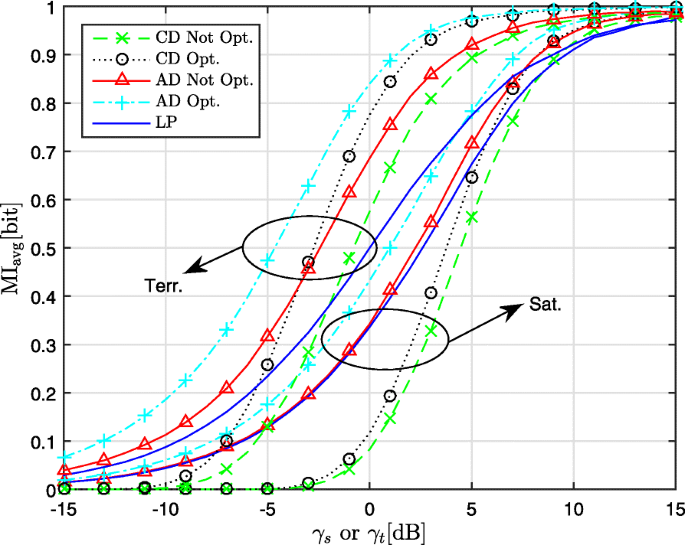
Performance of CD, AD and LP for 2-PAM on terrestrial and satellite channel
Fig. 6 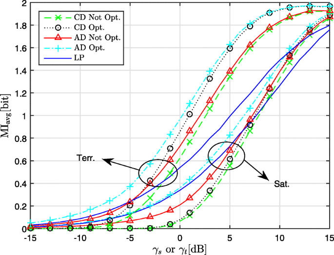
Performance of CD, AD and LP for 4-PAM on terrestrial and satellite channel
Fig. 7 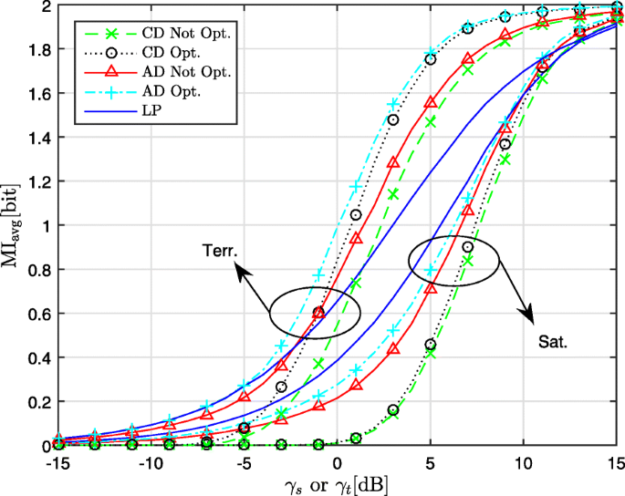
Performance of CD, AD, and LP for 4-QAM on terrestrial and satellite channel
-
For the terrestrial channel using the CD, TX optimization provides a larger gain than on the satellite channel. The curves for the optimized CD and the non-optimized AD intersect, with the latter outperforming the former in the lower range of MI, where the MoL of the non-optimized CD is large.
-
For both types of channel, the best performance is achieved by the optimized AD; the resulting gain compared to the non-optimized CD is largest for 2-PAM, because the fraction of the users that can remove the modulo operation is larger for 2-PAM than for 4-PAM and 4-QAM.


8.6 Comparison with LP
The LP is not affected by MoL and gives rise to a SNR at the detector given by:
Note that the performance resulting from LP is not affected by the user ordering nor the constellation rotations. If THP were without PoL, the corresponding SNR at the detector (10) would become
We have SNRdet,LP≤SNRdet,THP,noPoL, with equality if and only if the rows of H are orthogonal. In spite of this inequality, LP can outperform THP, when the latter is affected by a large amount of PoL and MoL.
We have included in Figs. 5, 6, and 7 also the average MI resulting from LP. Comparing the LP with the non-optimized CD for a given constellation, we observe that at large MI the non-optimized CD performs better, whereas the opposite occurs at low MI; this is because the MoL increases with decreasing MI, favoring LP at low MI. The crossing point, of the curves for LP and the non-optimized CD, occurs at larger MI for the satellite channel, compared to the terrestrial channel: the rows of H for the former channel tend to be more orthogonal (resulting in smaller interference), yielding a ratio SNRdet,LP/SNRdet,THP,noPoL closer to 1.
The optimized AD reduces the MoL and/or increases SNRdet,THP,noPoL of the THP scheme. On the terrestrial channel, the optimized AD outperforms LP over the entire range of MI and for all constellations considered. On the satellite channel, only for 2-PAM the optimized AD is the best over the entire range of MI; for 4-PAM and 4-QAM, LP outperforms the optimized AD for MI < 0.8 and MI < 1.5, respectively.
Figure 8 compares the different constellations considered, in terms of the maximum average MI over the LP and the optimized AD. For a given operating point, it can be seen from Figs. 5, 6, and 7 whether this maximum MI is achieved by the LP or by the optimized AD. The following observations can be made.
-
For the terrestrial channel, the best selection of constellations is (i) 2-PAM (with optimized AD) for MI <0.7; (ii) 4-PAM (with optimized AD) for 0.7 < MI <0.9; and (iii) 4-QAM (with optimized AD) for MI >0.9. In the interval 0.7 < MI <0.9, 4-PAM is only marginally better than either of 2-PAM and 4-QAM, so that only a small loss (less than 0.5 dB) is incurred when selecting 2-PAM for MI <0.8 and 4-QAM for MI >0.8 instead. According to Figs. 5, 6, and 7, the latter selection of constellations achieves a significant gain of up to about 4 dB, compared to the better of non-optimized CD and LP.
Fig. 8 
Best performance (over LP and optimized AD) for the different constellations on terrestrial and satellite channel
-
For the satellite channel, the best selection of constellations is (i) 2-PAM (with optimized AD) for MI <0.6; (ii) 4-QAM (with LP) for 0.6 < MI <1.5; and (iii) 4-QAM (with optimized AD) for MI >1.5. According to Figs. 5, 6, and 7, this optimum selection achieves only a moderate gain (up to about 1 dB) over the better of non-optimized CD and LP. Considering the higher complexity of the optimized AD, one might prefer to always use LP (with 2-PAM for MI <0.15 and 4-QAM for MI >0.15) instead.

From the above comparison, it follows that the channel statistics have a major impact on which algorithm and which constellation are optimum at a given MI: for the terrestrial channel, the optimized AD (combined with the proper constellation) provides the best performance over the entire range of MI, whereas the LP with 4-QAM performs best for the satellite channel over the medium range (0.6 < MI <1.5). This different behavior is attributed to the smaller interference on the satellite channel.
9 Conclusions
In this contribution, we consider a MU-MISO communication system with THP. The receiver uses a CD (always performing a modulo operation) or an AD (performing a modulo operation only when needed). We investigate the effect of reduced-complexity algorithms that select the symbol rotations at the TX and the ordering of the users, to reduce the MoL and to increase the SNR at the detector; several of these algorithms are novel.
Taking the average MI at the detector as a performance measure, results are presented for a terrestrial wireless channel and for a multi-beam satellite channel; we consider 2-PAM, 4-PAM, and 4-QAM constellations, since the PoL and MoL are the largest for small constellation sizes.
For the CD, the largest MI is obtained when the SNR at the detector is maximized, by selecting first the user ordering and then the rotations of the constellations; the latter step brings a substantial additional gain only for 2-PAM.
For the AD, no single algorithm is optimum for the entire range of MI; as the MoL is larger for small MI, the better algorithms are those which reduce the MoL for small MI and increase the SNR at the detector for large MI. When optimizing the TX, the gains resulting from the AD are considerably larger than those from the CD, especially at small MI (where the MoL of the CD is large); hence, the AD with TX optimization outperforms the CD with TX optimization. These gains are larger for 2-PAM than for 4-PAM and 4-QAM, mainly because the optimization of the constellation rotations has a larger effect for 2-PAM.
When selecting the best constellation for the optimized AD and for the LP, it is found that, on the terrestrial channel, the optimized AD outperforms the LP; compared to the better of LP and non-optimized CD, the optimized AD achieves a significant gain (up to about 4 dB). In contrast, on the satellite channel, the optimized AD actually performs worse than the LP for the medium range of MI and achieves only a modest gain (up to about 1 dB) for small and large MI. Hence, the application of the optimized AD is quite promising for wireless terrestrial communication, whereas its usefulness for multi-beam satellite communication is rather limited.
Although the focus of this contribution is on MU-MISO THP, the concepts are easily extended to SU-MIMO and MU-MIMO scenarios.
Notes
When condition C(n) holds, it does not matter whether or not the modulo operation at the TX is active for the n-th user. Hence, from a practical point of view, having the modulo operation at the TX active for all NU users is the simplest choice.
The algorithm from [14] maximizes SNRdet for the CD, with \(\sigma _{\mathrm {mod,n}}^{2}\) computed as an arithmetical average over a block of transmitted data, instead of an expectation over the data. Both approaches yield similar results for long frames.
We make abstraction of the 0.02 dB higher SNR gain at MI = 0.3 for (MoL,P)RC compared to (MoL+SNR,P)RC, which is negligible and might be caused by limited numerical accuracy.
Abbreviations
- AD:
-
Alternative detector
- CCI:
-
Co-channel interference
- CD:
-
Conventional detector
- CSI:
-
Channel state information
- DPC:
-
Dirty paper coding
- FSL:
-
Free space loss
- LOS:
-
Line of sight
- LP:
-
Linear precoding
- MI:
-
Mutual information
- MIMO:
-
Multiple-input multiple-output
- MISO:
-
Multiple-input single-output
- MoL:
-
Modulo loss
- MU:
-
Multi-user
- PAM:
-
Phase amplitude modulation
- PoL:
-
Power loss
- QAM:
-
Quadrature amplitude modulation
- RC:
-
Reduced-complexity
- RX:
-
Receiver
- SNR:
-
Signal-to-noise ratio
- SU:
-
Single-user
- THP:
-
Tomlinson-Harashima precoding
- TX:
-
Transmitter
- ZF:
-
Zero-forcing
References
M. H. M. Costa, Writing on dirty paper. IEEE Trans. Inform. Theory. IT-29:, 439–441 (1983).
M. Tomlinson, New automatic equalizer employing modulo arithmetic. Lett. 7(5), 138–139 (1971).
H. Harasima, H. Miyakawa, Matched-Transmission Technique for Channels with Intersymbol Interference. IEEE Trans. Commun. COM-20:, 774–780 (1972).
R. F. H. Fischer, C. Windpassinger, A. Lampe, J. B. Huber, Tomlinson-Harashima precoding in space-time transmission for low-rate backward channel. Int. Zurich Semin. Broadband Commun. Access Transm. Netw. 1–6 (2002).
C. Windpassinger, T. Vencel, R. F. H. Fischer. Precoding and loading for BLAST-like systems. IEEE Int. Conf. Commun. (ICC). 3061–3065 (2003).
F. S. Tseng, B. G. Sun, Sensitivity Analysis for RVQ- Based Tomlinson-Harashima Precoded MIMO Systems. IEEE Trans. Veh. Technol. 65(2), 978–985 (2016).
R. F. H. Fischer, C. A. Windpassinger, MIMO Improved. precoding for decentralized receivers resembling concepts from lattice reduction. IEEE Glob. Telecommun. Conf. (GLOBECOM). 1852–1856 (2003).
K. Kusume, M. Joham, W. Utschick, G. Bauch, Efficient Tomlinson-Harashima Precoding for Spatial Multiplexing on Flat MIMO Channel. IEEE Int. Conf. Commun. 3:, 2021–2025 (2005).
W. Yu, D. P. Varodayan, J. M. Cioffi, Trellis and convolutional precoding for transmitter-based interference presubtraction. IEEE Trans. Commun. 53(7), 1220–1230 (2005).
R. Habendorf, G. Fettweis, On Ordering Optimization for MIMO Systems with Decentralized Receivers. Vehicular Technology Conf (VTC), 1844–1848 (2006).
F. A. Dietrich, P. Breun, W. Utschick, Robust Tomlinson–Harashima precoding for the wireless broadcast channel. IEEE Trans. Signal Proc. 55(2), 631–644 (2007).
J. Liu, W. A. Krzymien, A Novel Nonlinear Precoding Algorithm for the Downlink of Multiple Antenna Multi-User Systems. Wirel. Pers. Commun. 207–223 (2007).
K. Kusume, M. Joham, W. Utschick, G. Bauch, Cholesky factorization with symmetric permutation applied to detecting precoding spatially multiplexed data streams. IEEE Trans. Signal Proc. 55(6), 3089–3103 (2007).
J. Kang, H. Ku, D. S. Kwon, C. Lee, Tomlinson-Harashima precoder with tilted constellation for reducing the transmission power. IEEE Trans. Wirel. Comm. 8(7), 3658–3667 (2009).
C. Masouros, M. Sellathurai, T. Ratnarajah, Interference Optimization for Transmit Power Reduction in Tomlinson-Harashima Precoded MIMO Downlinks. IEEE Trans. Sig. Process. 60(5), 2470–2481 (2012).
L. Sun, M. R. McKay, Tomlinson-Harashima Precoding for Multiuser MIMO Systems With Quantized CSI Feedback and User Scheduling. IEEE Trans. Sig. Process. 62(16), 4077–4090 (2014).
E. Debels, A. Suls, M. Moeneclaey, in IEEE Symposium on Commun. and Vehicular Techn. in the Benelux (SCVT). Modulo loss reduction in spatial multiplexing systems with Tomlinson-Harashima precoding (IEEELuxembourg, 2015).
E. Debels, A. Suls, M. Moeneclaey, Modulo loss reduction for Tomlinson-Harashima precoding in a multi-beam satellite forward link. IEEE Int. Work. Sign. Process. Adv. Wirel. Commun. (SPAWC), 5 (2016).
K. Zu, R. C. de Lamare, M. Haardt, Multi-Branch Tomlinson-Harashima Precoding Design for MU-MIMO Systems: Theory and Algorithms. IEEE Trans. Commun. 62(3), 939–951 (2014).
X. Geng, B. An, F. Liu, F. Cao, Robust THP Transceiver Design for MIMO Interference Channel. IEEE Commun. Lett. 19(9), 1640–1643 (2015).
L. Sun, J. Wang, V. Leung, Joint Transceiver, Data Streams, and User Ordering Optimization for Nonlinear Multiuser MIMO Systems. IEEE Trans. Commun. 63(10), 3686–3701 (2015).
X. Lu, R. C. de Lamare, K. Zu, Successive optimization Tomlinson-Harashima precoding strategies for physical-layer security in wireless networks. J. Wirel. Com. Netw. 259(2016), 1–12 (2016).
Q. Li, Q. Zhang, J. Qin, Robust Tomlinson-Harashima Precoding With Gaussian Uncertainties for SWIPT in MIMO Broadcast Channels. IEEE Trans. Signal Process. 65(6), 1399–1411 (2017).
P. W. Wolniansky, G. J. Foschini, G. D. Golden, R. A. Valenzuela, V-BLAST: an architecture for realizing very high data rates over the rich-scattering wireless channel. IEEE Int. Symp. Signals Syst. Electron. (ISSSE). 295–300(1998).
D. Wubben, J. Rinas, R. Bohnke, V. Kuhn, K. D. Kammeyer, in 4th International ITG Conference on Source and Channel Coding. Efficient Algorithm for Detecting Layered Space-Time Codes (IEEEBerlin, 2002).
M. Diaz, N. Courville, C. Mosquera, G. Liva, G. Corazza, in IEEE Intern. Workshop on Satellite and Space Commun. (IWSSC). Non-Linear Interference Mitigation for Broadband Multimedia Satellite Systems (IEEESalzburg, 2007), pp. 61–65.
M. Poggioni, M. Berioli, P. Banelli, in IEEE International Conf. on Commun. BER performance of Multibeam Satellite Systems with Tomlinson-Harashima Precoding (IEEEDresden, 2009), pp. 1–6.
P. Arapoglou, K. Liolis, M. Bertinelli, A. Panagopoulos, P. Cottis, R. De Gaudenzi, MIMO over satellite: A Review. IEEE Commun. Surv. Tutorials. 13(1), 27–50 (2011).
F. Lombardo, E. A. Candreva, I. Thibault, A. Vanelli-Coralli, G. E. Corazza, in 2011 Conference Record of the Forty-Fifth Asilomar Conference on Signals, Systems and Computers (ASILOMAR). Multi-user interference mitigation techniques for broadband multi-beam satellite systems (IEEEPacific Grove, 2011), pp. 1805–1809.
J. Arnau, B. Devillers, C. Mosquera, A. Perez-Neira, Performance study of multiuser interference mitigation schemes for hybrid broadband multibeam satellite architectures (Springer International Publishing, 2012). 05 April 2012, https://doi.org/10.1186/1687-1499-2012-132.
G. Zheng, S. Chatzinotas, B. Ottersten, Generic Optimization of Linear Precoding in Multibeam Satellite Systems. IEEE Trans. Wirel. Commun. 11(6), 2308–2320 (2012).
V Boussemart, L Marini, M Berioli, in 6th Advanced Sat. Multimedia Syst. Conf. (ASMS) and 12th Signal Proc. for Space Commun. Workshop (SPSC). Multi-Beam Satellite MIMO Systems: BER Analysis of Interference Cancellation and Scheduling (IEEEBaiona, 2012), pp. 197–204.
J Arnau, C Mosquera, in IEEE 6th Advanced Sat. Multimedia Systems Conf. (ASMS) and 12th Signal Proc. for Space Comm. Workshop (SPSC). Performance Analysis of Multiuser Detection for Multibeam Satellites Under Rain Fading (IEEEBaiona, 2012), pp. 212–219.
G. Maral, M. Bosquet, Satellite communications systems, 4th ed (Wiley, 2002). ISBN 0471496545, 9780471496540.
J. Mazo, J. Salz, On the Transmitted Power In Generalized Partial Response. IEEE Trans. Commun. 24(3), 348–352 (1976).
T. M. Cover, J. A. Thomas, Elements of information theory (Wiley-Interscience, New York, 1991).
Funding
This work was supported by the Research Foundation Flanders (FWO) under grant no. EOS-30452698.
Author information
Authors and Affiliations
Contributions
ED conceived the study, designed the novel algorithms, performed the simulation experiments, and drafted the manuscript. MM reviewed and edited the manuscript. Both authors read and approved the final manuscript.
Corresponding author
Ethics declarations
Competing interests
The authors declare that they have no competing interests.
Publisher’s Note
Springer Nature remains neutral with regard to jurisdictional claims in published maps and institutional affiliations.
Additional information
Authors’ information
E. Debels is currently pursuing the PhD degree at Ghent University. M. Moeneclaey is Full Professor at Ghent University.
Rights and permissions
Open Access This article is distributed under the terms of the Creative Commons Attribution 4.0 International License (http://creativecommons.org/licenses/by/4.0/), which permits unrestricted use, distribution, and reproduction in any medium, provided you give appropriate credit to the original author(s) and the source, provide a link to the Creative Commons license, and indicate if changes were made.
About this article

Cite this article
Debels, E., Moeneclaey, M. SNR maximization and modulo loss reduction for Tomlinson-Harashima precoding. J Wireless Com Network 2018, 257 (2018). https://doi.org/10.1186/s13638-018-1262-7
Received:
Accepted:
Published:
DOI: https://doi.org/10.1186/s13638-018-1262-7