- Research
- Open access
- Published:
Fast design of multiband fractal antennas through a system-by-design approach for NB-IoT applications
EURASIP Journal on Wireless Communications and Networking volume 2019, Article number: 68 (2019)
Abstract
The efficient design of compact antennas operating over multiple bands suitable for the Internet of Things (IoT) is addressed by means of an instance of the system-by-design (SbD) paradigm. More specifically, an iterative strategy that combines different software modules for the search spaceexploration, the fast physicalmodeling of the radiators, and the quality evaluation of the guess solutions is proposed. To enable such a SbD instance, an innovative strategy that exploits an orthogonal array (OA) scheme to determine the training set of a Learning-by-Example (LBE) algorithm based on a support vector regressor (SVR) is introduced for the efficient physicalmodeling of the layout to be optimized. The features and the potentialities of the proposed methodological approach are assessed in different applicative scenarios by considering representative numerical and experimental validation examples.
1 Introduction and rationale
Nowadays, the ever-growing development of the Internet of Things/Internet of Everything (IoT/IoE) is rapidly pushing the concept of “pervasive intelligence” [1–3] to an unprecedented level, in which several small and relatively cheap objects of our daily lives will be densely interconnected through wireless machine-to-machine (M2M) interactions [4]. Within this context, 3GPP recently released in June 2016 the first version of the NarrowBand-IoT (NB-IoT) [5, 6]. NB-IoT is an emerging new wireless access technology, which will exist together with the other existing cellular networks like GSM, UMTS, and LTE. The main concept from 3GPP standards is the integration of NB-IoT with current LTE networks. Clearly, several heterogeneous communication (e.g., WLAN [7], WI-MAX [8], Bluetooth [9], UMTS [10], LTE [11], 5G [12, 13]), tagging (RFID, NFC) [14], and localization (GPS, GALILEO) [15] services will have to be suitably hosted/integrated onto a single device to make the IoT/IoE vision feasible in the next few years. Multiband antennas are a brilliant technological solution to reach this goal, while minimizing the size of the RF front-end [16]. However, standard antennas (e.g., dipoles, loops, square patches) cannot be easily tuned to simultaneously support wireless standards arbitrarily located in the frequency spectrum [16, 17]. Moreover, the constraints on the size, the fabrication technology, the costs, and the antenna robustness further complicate the design problems at hand [17]. To properly address these issues, several different technological/algorithmic approaches for the synthesis of multi-band radiators for mobile terminals have been proposed and they are still under development. In this framework, microstrip printed antennas with perturbed fractal shapes have been considered as a viable solution to yield low-profile and low-cost antennas operating over multiple independent bands [18–24]. As a matter of fact, although self-similarity properties of standard/unperturbed fractal shapes enable antennas to exhibit a multi-band behavior [16, 25–33], fractals with perturbed geometry proved to be more flexible since they can effectively break the fixed relationships among working resonances [23]. Despite its effectiveness, the underlying design procedure is often extremely cumbersome from the numerical viewpoint. As a matter of fact, nowadays synthesis techniques are based on iterative optimization techniques derived from Evolutionary Algorithms (EAs) [34–37] combined with full-wave antenna simulators. However, it cannot be neglected that in such schemes, each guess solution (i.e., an antenna configuration) must be evaluated through a full-wave simulator [18–23] and the computation time to yield the final design can easily diverge. Moreover, any new antenna design is obtained as the result of an independent synthesis process.
To overcome the above limitations, this work presents a new multi-band antenna design concept as a complement and generalization of existing design methodologies. An instance of the system-by-design (SbD) paradigm [38–40] is introduced for the numerically efficient and scalable synthesis of multi-band microstrip printed antennas based on perturbed fractal shapes. The key motivation for this choice is that the SbD paradigm, which is defined as “a functional ecosystem to handle complexity in the design of large systems,” enables the formulation of arbitrary design problems in a modular way so that each module (block) of the synthesis process solves a simple task and it can be replaced by a functionally equivalent one on the basis of the design needs, objectives, constraints, and degrees-of-freedom (DoFs). More specifically, the SbD paradigm is here applied to define a design procedure (Fig. 1) that integrates (a) an effective solution-space search (SSS) functional block aimed at iteratively generating a sequence of guess solutions (i.e., perturbed fractal geometries) that converges towards an optimal antenna geometry fitting the problem constraints; (b) a physical response emulator (PRE) block devoted to the fast computation/modelling of the electrical/radiating behavior of each guess radiator; and (c) a physical objective assessment (POA) block responsible for the evaluation of the “quality” (i.e., the matching of the design objectives) of each trial design. Accordingly, the aim of this paper is to present a novel methodology based on the suitable customization of the SbD functional blocks towards a flexible and computationally efficient synthesis of perturbed microstrip fractal antennas.

SbD design procedure flowchart
As for the former functional block (SSS block; Fig. 1), iterative global optimization methods turn out to be suitable tools for handling the DoFs of the antenna design (i.e., its geometrical descriptors) and the non-convex synthesis problem at hand [34–37]. The POA block is mathematically defined by specifying a “cost function” quantifying the mismatch between the response of each trial solution and the project constraints and requirements. Designing a suitable PRE block is a more challenging task. Indeed, the most natural choice of using a full-wave EM solver for predicting the electromagnetic behavior of each guess solution is generally avoided because of the resulting computational costs. Otherwise, Learning-by-Example (LBE) strategies [41] based on support vector regressors (SVRs) [42] represent a suitable candidate alternative. These methods, which have solid mathematical foundations in statistical learning theory [42], are two-step procedures based on an (off-line) “training phase,” where a set of input-output examples are provided to let the SVR “learn” the corresponding physical relations, and a “testing phase,” where the SVR is used to emulate the full-wave solver predicting in real-time the physical response of the system [41, 42]. However, the effective application of such approaches requires the off-line generation of a “representative” training set whose cardinality is proportional to the number of DoFs of the problem at hand. Of course, building the training set by enumerating every possible combination of the control parameters turns out numerically unfeasible since the number of different training configurations would grow exponentially with the number of DoFs [43]. To overcome such a bottleneck, orthogonal arrays (OAs) are here chosen as an enabling tool for exploiting LBE techniques since they allow to enforce the training ensemble to span the search space uniformly (i.e., sampling each design parameter with the same accuracy), while minimizing its size [43–45].
Accordingly, the main novelty of this paper consists in (i) the introduction of a scalable synthesis tool, which can be efficiently re-used for several different objectives/designs, since the off-line training phase for the electromagnetic prediction is done only once for each class of reference antenna geometry (e.g., Sierpinski, Hilbert, Koch fractal patches); (ii) the first attempt to exploit the OA features to build an optimal training set with reduced cardinality to enhance and speed-up the SVR training phase; and (iii) the first customization of the SbD building blocks to efficiently and effectively deal with the synthesis of multi-band microstrip antennas.
The paper is organized as follows. The multiband antenna synthesis problem at hand is mathematically stated in Section 2, while the SbD design approach is detailed in Section 3. A set of numerical and experimental assessments is then reported to give the interested reader some insights on the key features and the potentialities of the proposed design approach (Section 4). Some concluding remarks will follow (Section 5).
2 Synthesis problem formulation
Let us consider a generic structure composed of a perturbed fractal metallic layer printed on a dielectric substrate of thickness h characterized by a relative dielectric permittivity εr and a dielectric loss tangent tanδ, and backed by a metallic ground-plane. By describing such a geometry by means of the feature vector g={gp, p=1,...,P} containing all the P (real-valued) design parameters or problem DoFs (i.e., fractal dimensions, feed shape, substrate width and height), the antenna synthesis problem at hand can be stated as follows:
Multiband antennasynthesis problem—set the values of the unknown entries of g within the user-defined DoF boundaries such that \(s_{11}\left (f;\mathbf {g}\right)\leq s_{11}^{th}\) for all f∈{fn, n=1,...,N}
s11(f;g) being the antenna scattering parameter at the frequency f and \(s_{11}^{th}\) the corresponding user-defined constraint/requirement. Moreover, N is the number of bands of interest and fn is the central frequency of the n-th (n=1,...,N) band. Of course, such a statement as well as the corresponding problem can be easily extended to include additional constraints (e.g., mechanical, thermal, and chemical features) by adding suitable constraint terms. However, the generalization of the antenna synthesis to multi-physics formulations is beyond the scope of the current work and it will not be discussed in the following.
3 SbD synthesis procedure
3.1 Statement of SbD problem
Following the SbD approach [38–40] pictorially summarized in Fig. 1, the multiband antenna synthesis problem is re-formulated as the following optimization one:
System-by-design multiband antenna synthesis problem—find gopt= ming[Φ(g)]such that \(\mathbf {g}\in \mathcal {G}\)
where \(\mathcal {G}=\left \{\left [g_{p}^{\min },g_{p}^{\max }\right ],\, p=1,...,P\right \} \) is the DoF feasibility region accounting for technological and/or physical constraints and Φ(g) is the cost function of the synthesis problem:
quantifying the mismatch with the project requirements, \(\widehat {f}_{n}\left (\mathbf {g}\right)\) being the n-th resonant frequency [i.e., the central frequency of the n-th band for which \(s_{11}\left (f_{n};\mathbf {g}\right)\leq s_{11}^{th}\)] of the multiband antenna with geometry descriptors g.
To solve such a problem, the iterative SbD procedure in Fig. 1 is exploited. It comprises the following elementary functional blocks:
-
A SSS block that generates, according to a suitable global optimization strategy, the guess solutions (i.e., perturbed fractal shapes coded into trial vectors g) convergent to the optimal antenna configuration gopt
-
A PRE block aimed at estimating the resonant frequencies \(\widehat {f}_{n}\left (\mathbf {g}\right)\), n=1,...,N of the SSS-block-generated guess geometry g by means of a computationally effective “forward” strategy
-
a POA block that evaluates the matching between the desired and the resonant frequencies of the trial multiband antenna, g, by computing the value of Φ(g), which takes into account also the physical/application constraints
It is worth pointing out that the modularity of the scheme in Fig. 1 represents one of the most important features of the SbD paradigm. As a matter of fact, it enables the choice of the most suitable tool to perform each sub-task of the SbD loop by fully exploiting the interrelations among the blocks [38–40]. As a consequence, the different functionalities can act as mutual enablers for the selection of the most suitable techniques to be adopted, depending on the applicative constraints and objectives [38–40]. As concerns the multiband antenna synthesis, the POA block is straightforwardly implemented since its definition requires the evaluation of (1) and the assessment of the membership of the trial solution to the DoF feasibility region \(\mathcal {G}\). Conversely, the implementations of the PRE block (Section 3.2) and the SSS block (Section 3.3) need to be carefully addressed, and they will be detailed in the following sub-sections.
3.2 PRE block
Due to the computational constraints in effectively using an iterative global optimization, a LBE approach is adopted for the PRE block implementation [41]. More specifically, an algorithm derived from SVR [42] is considered. After an off-line training phase performed to learn the input-output relations of the system to be emulated (Section 3.2.1) starting from a set of T training set couples \(\left [\mathbf {g}^{(t)},\,\widehat {f}_{n}\left (\mathbf {g}^{(t)}\right)\right ], t=1,...,T, n=1,...,N\), a fast online testing phase is then carried out to emulate the physical system itself (Section 3.2.2). Towards this end, the relation between the estimated resonant frequencies, \(\widehat {f}_{n}\left (\mathbf {g}\right)\), n=1,...,N, and the antenna parameters g is modelled as [46]:
where \(\mathcal {K}\left (\cdot,\cdot \right)\) is the so-called kernel functionFootnote 1, \(\boldsymbol {\alpha }_{n}\triangleq \left \{ \alpha _{n}^{(t)};\, t=1,...,T\right \} \) and \(\boldsymbol {\beta }_{n}\triangleq \left \{ \beta _{n}^{(t)};\, t=1,...,T\right \} \), n=1,...,N, are the SVR weights, and bn is the offset for the n-th frequency.
3.2.1 Off-line SVR phase
In order to define the training set (i.e., \(\left \{\left [\mathbf {g}^{(t)},\,\widehat {f}_{n}\left (\mathbf {g}^{(t)}\right)\right ];\right. \left. t=1,...,T; n=1,...,N\text {l}{\vphantom {\left [\mathbf {g}^{(t)},\,\widehat {f}_{n}\left (\mathbf {g}^{(t)}\right)\right ]}}\right \}\)), an OA approach [43, 44, 47] is adopted to determine the representative sample points, {g(t),t=1,...,T}, of the domain of the functional space, {\(\widehat {f}_{n}\left (\mathbf {g}\right)\); n=1,...,N} to be estimated through LBE. Indeed, it is well known that such a method allows one to statistically sample the space \(\mathcal {G}\) in a uniform way, while also minimizing the size T of the training set [43, 44, 47]. More in detail, the t-th (t=1,...,T) input training sample is defined as:
where
and ωtp is the t,p-element of a (L,T,P)-OA
The entries of Ω are built so that they can assume an integer value within the range [0,L−1], L being the number of quantization steps (i.e., levels) chosen to discretize each parameter gp, p=1,...,P, in the sampling space \(\mathcal {G}\). Moreover, the following properties hold true [47]:
-
1
Any (discrete) value of ωtp appears \(\frac {T}{L}\) times in any column t of Ω (t=1,...,T).
-
2
Any couple of (discrete) values (ωtp,ωrp) appears \(\frac {T}{L^{2}}\) times in any couple of columns (t,r) of Ω (t=1,...,T; r=1,...,T).
-
3
A matrix \(\widetilde {\Omega }\) obtained by swapping the columns of Ω is still an OA.
-
4
A matrix \(\widetilde {\Omega }\) obtained by taking away some of the columns of Ω is still an OA.
For illustrative purposes, let us consider the (L,T,P)-OA Ω with L=3,P=4,T=9 reported in Table 1 [48]. As it can be noticed, the entries are integers belonging to the range [0,L−1]=[0,2]. Moreover, the matrix Ω satisfies the OA properties: (Property 1) the value “0” appears \(\frac {T}{L}=3\) times in any column of Ω and the same holds true for the values “1” and “2”; (Property 2) the couple “22” appear \(\frac {T}{L^{2}}=1\) times for each couple of columns of Ω and the same holds true for each couple of values; the same properties are satisfied also by swapping the columns of Ω (Property 3) and by removing some of them (Property 4).
Since the OA sampling is best rule for representing a LP-size feasibility space with T uniformly located points, the optimal SVR training samples are computed through (3) by referring to an (L,T,P)-OA Ω matrix either available in online OA repositories [48] or built according to the procedures described in [47] (see the Appendix).
Once the set of input training samples, { g(t),t=1,...,T}, is determined by means of (3), the computation of the associated resonance frequencies, {\(\widehat {f}_{n}\left (\mathbf {g}^{(t)}\right); t=1,...,T, n=1,...,N\)} (i.e., the output training samples), is at hand to complete the definition of the training set {\(\left [\mathbf {g}^{(t)},\,\widehat {f}_{n}\left (\mathbf {g}^{(t)}\right)\right ]\); t=1,...,T, n=1,...,N}. Towards this end, T full-wave electromagnetic simulations are carried out with a Method-of-Moments (MoM) technique to determine the values of s11(f;g(t)), t=1,...,T.
The training phase is completed by determining the optimal values of the ε-SVR parameters (i.e., \(\boldsymbol {\widetilde {\alpha }}_{n}\triangleq \left \{\widetilde {\alpha }_{n}^{(t)};\, t=1,...,T\right \} \), \(\boldsymbol {\widetilde {\beta }}_{n}\triangleq \left \{\widetilde {\beta }_{n}^{(t)};\, t=1,...,T\right \} \), and \(\widetilde {b}_{n}, n=1,...,N\) [46]). Accordingly, the following minimization problem is solved:
by means of a local minimization strategy based on the Sequential Minimal Optimization approach proposed in [46]. Afterwards, the Karush-Kuhn-Tucker condition is exploited to estimate \(\widetilde {b}_{n}\) (n=1,...,N) (see [46], Section 4.1.5). In (6), Q= {\(q_{tr}=\mathcal {K}\left (\mathbf {g}^{(t)},\mathbf {g}^{(r)}\right)\); t=1,...,T; r=1,..,T} is the kernel matrix, ε and C are user-defined control parameters, and ·′ stands for the transpose operator.
3.2.2 Online SVR phase
Once \(\left (\boldsymbol {\widetilde {\alpha }}_{n},\,\boldsymbol {\widetilde {\beta }}_{n},\,\widetilde {b}_{n}\right)\), n=1,...,N, have been computed by means of (6), the online SVR phase is carried out by simply substituting the desired g in (2) and enforcing \(\boldsymbol {\alpha }_{n}\leftarrow \boldsymbol {\widetilde {\alpha }}_{n}\), \(\boldsymbol {\beta }_{n}\leftarrow \boldsymbol {\widetilde {\beta }}_{n}\), and \(b_{n}\leftarrow \widetilde {b}_{n}\) [46]. Thus, a simple and very fast function evaluation is needed to emulate the physical response (resonance frequencies) of each guess antenna configuration instead of recurring to a computationally heavy full-wave MoM simulation. On the other hand, it is worth pointing out that such a feature is a key asset for the integration of the PRE block within the SbD design loop (Fig. 1). Indeed, since the physical response of an antenna can be evaluated in a very efficient manner, the PRE block acts as an enabler for SSS blocks based on iterative search strategies [e.g., multi-agents global optimizers based on EAs (Section 3.3)] requiring the evaluation of a huge number of guess solutions. Moreover, the off-line training phase (6) needs to be performed only once for each antenna typology (i.e., fractal shape); thus, such a PRE block can be re-used in various SbD procedures concerned with different applicative scenarios, even though still dealing with fractal shapes, as proved in Section 4 through some representative experiments.
3.3 SSS block
As for the SSS block, it is required that the underlying methodology complies with the applicative constraints and the features of the other functional tools involved in the SbD loop (Fig. 1) [38–40]. More specifically, it must be able to (i) properly handle the type of design variables of interest (i.e., real-valued g), (ii) effectively sample the solution space by avoiding to be trapped in local minima during the iterative searching procedure, and (iii) enable the definition of arbitrary cost functions, Φ(g), and physical constraints, \(\mathcal {G}\), for the design of interest. Because of the features of the multiband antenna problem at hand, a global optimization based on EAs [35] is adopted. More specifically, the real-valued nature of g and the (potentially) large number of parameters P describing the antenna geometry suggest the use of a particle swarm (PS) optimizer [35]. Accordingly, the inertial-weight version of the PS with reflecting boundary condition is considered [35]. The iterative procedure, which generates an optimal guess solution \(\mathbf {g}_{i}^{opt}\) at each iteration i, is stopped when one of the following conditions is met:
-
A maximum number of iterations I is reached (i.e., i=I,I being an user-defined iteration number)
-
The fitness reaches stationarity
$$ I_{win}\Phi\left(\mathbf{g}_{i}^{opt}\right)-\sum_{v=1}^{I_{win}}\Phi\left(\mathbf{g}_{i-v}^{opt}\right) \leq\eta\Phi\left(\mathbf{g}_{i}^{opt}\right) $$(7)η and Iwin being a user-defined stagnation threshold and an iteration window, respectively
-
The fitness value is smaller than a user-defined threshold value, \(\zeta \left [\text {i.e.}, \Phi \left (\mathbf {g}_{i}^{opt}\right)\leq \zeta \right ]\)
It is worth remarking that the proposed SbD approach can be applied without restrictions on the multi-frequency antenna geometry, constraints, and objectives, provided that \(\mathbf {g}, \mathcal {G}\), and Φ(·) are properly defined and the T training samples \(\left [\mathbf {g}^{(t)},\,\widehat {f}_{n}\left (\mathbf {g}^{(t)}\right)\right ]\), t=1,...,T are computed. This is a key advantage of the SbD paradigm over standard design methodologies since it also guarantees the re-usability of the majority of the SbD modules across different synthesis problems.
4 Numerical and experimental results
This section is aimed at illustrating both the off-line (Section 4.1) and the online (Section 4.2) phases of the proposed SbD approach, as well as assessing its effectiveness through an experimental validation (Section 4.3). Towards this end, the design of a dual-band (N=2) Sierpinski Gasket fractal shape [27] shown in Fig. 2 is assumed as a benchmark example. In such a case, the feature vector g is characterized by P=9 entries encoding the geometric descriptors in Fig. 2: \(g_{1}=w_{a}, g_{2}=h_{a}, g_{3}=w_{1}, g_{4}=w_{2}, g_{5}=h_{f}, g_{6}=h_{g}, g_{7}=\frac {w_{3}}{W_{3}}, g_{8}=\frac {w_{4}}{W_{4}}\), and \(g_{9}=\frac {w_{5}}{W_{5}}\). Concerning the substrate properties, an Arlon layer with εr=3.38, tanδ=0.0025, and h=7.6×10⁻⁴ [m] has been considered. For comparison purposes, all the computational costs refer to a non-optimized Matlab implementation of the methodology running on a desktop PC with a 2.6 GHz single-core processor.

Problem geometry. Perturbed planar Sierpinsky Gasket fractal antenna and antenna descriptors: (a) front and (b) back views
4.1 Off-line training of the PRE block
As for the off-line phase of the PRE block, the definition of the training set \(\left [\mathbf {g}^{(t)},\,\widehat {f}_{n}\left (\mathbf {g}^{(t)}\right)\right ], t=1,...,T, n=1,...,N\) requires the choice of the suitable OA Ω for the problem at hand. Towards this end, L=61 quantization levels for the antenna descriptors have been considered to carefully discretize the entire search space \(\mathcal {G}\). The auxiliary OA \(\Omega ' \triangleq \) {\(\omega _{tp}'\in \mathbb {N}\cap \left [0,L-1\right ]\); t=1,...,T,p=1,...,P′} has been determined by following the procedure in [47] yielding J=2, T=LJ=3721, \(P'=\frac {L^{J}-1}{L-1}=62\) (see the Appendix). The training OA Ω has been successively identified by deleting the last P′−P=53 columns of Ω′ by enforcing:
Once Ω has been defined, Eq. (3) has been used to compute the T input training samples { g(t); t=1,...,T} by setting the range of the antenna descriptors (i.e., \(\mathcal {G}\); Table 2) according to the guidelines discussed in [21] so that the resonating frequencies fall within the band of interest for IoT/IoE communications. The resonant frequencies, {\(\widehat {f}_{n}\left (\mathbf {g}^{(t)}\right)\); t=1,...,T; n=1,...,N} in correspondence with the input set { g(t); t=1,...,T}, have been computed through a full-wave solver Footnote 2 by setting \(s_{11}^{th}=-10\) [dB]. As it can be observed (Fig. 3), there are several training samples characterized by a dual-band behavior (i.e., two resonances) in the [1.0−6.0] GHz range [i.e., \(s_{11}\left (f_{n}\left (\mathbf {g}^{(t)}\right);\,\mathbf {g}^{(t)}\right)\leq s_{11}^{th}\), n=1,2]. Of course, different bandwidths could be easily covered by suitably scaling \(\mathcal {G} \left [\text {i.e.}, f_{n}\left (\mathbf {g}\right)\to \frac {f_{n}\left (\mathbf {g}\right)}{10} \text {then}\ \mathcal {G}\to \frac {\mathcal {G}}{10}\right ]\).

PRE block (SVR training). Plot of \(\widehat {f}_{n}\left (\mathbf {g}^{(t)}\right), n=1,..,N, t=1,...,T\) of the T=3721 OA-defined training samples (n=1→ blue cross; n=2→ green cross)
Concerning the SVR implementation, a radial basis function (RBF) kernel has been adopted [46]:
fixing to γ=0.1 [46] the value of the RBF control parameter γ. To complete the off-line phase of the PRE block, Eq. (6) (i.e., the SVR training) has been solved by using the procedure in Section 3.2.1 and enforcing the control parameters to ε=0.01 and C=1 as suggested in [46]. It is worth pointing out that such a PRE block allows one to estimate the output values {\(\widehat {f}_{n}\left (\mathbf {g}\right)\); n=1,..,N} through (2) in about:
while the same result would require about ΔtMoM≈2.7×10²[s] using a standard MoM code for simulating the same antenna configuration, g.
4.2 Numerical assessment
The first numerical experiment is aimed at illustrating, on a step-by-step basis, the exploitation of the proposed integrated SbD procedure (Fig. 1) for designing a dual-band antenna working at the LTE-2100 (f1=2.045 GHz) and the LTE-3500 (f2=3.5 GHz) channels. Towards this end, the PRE block (Section 4.1) has been combined with the POA block (1) and the PS-based SSS block configured by following the guidelines in [21, 35]: S=8, ζ=10−10, I=200, η=10−4, and Iwin=30. The plot of the “global best” value of the cost function, \(\Phi _{i}\triangleq \Phi \left (\mathbf {g}_{i}^{opt}\right)\), versus the iteration index, i, in Fig. 4(a) shows that the method converges in about Iconv≈100 iterations Footnote 3, which correspond to Iconv×S=800 cost function evaluations requiring ΔtSbD≈800×ΔtPRE=0.8 [s]. The comparison with the computational cost of a standard optimization loop remarks the efficiency of the PRE block implementation and the whole SbD design procedure. As a matter of fact, the same process adopting a simulation block based on a MoM solver would have taken about Δtstandard≈800×ΔtMoM≈2.16×10⁵ [s]. On the other hand, the accuracy of the PRE emulation is assessed by the plots of the simulated scattering parameter Footnote 4 of the optimized layout (Fig. 4b). As a matter of fact, despite the emulation of the physical response of the antenna, the synthesized antenna profile (Fig. 5a–b) perfectly matches the design objectives expressed in terms of impedance matching in the operating bands (i.e., \(s_{11}\left (f;\mathbf {g}\right)\leq s_{11}^{th}=-10\) dB, f∈{fn, n=1,...,N}={2.045, 3.5} GHz; Fig. 4b). As for the radiation properties, the simulated 3D gain patterns computed at fn, n=1,...,N indicate that the antenna exhibits a dipole-like behavior (e.g., fn=2.045 GHz; Fig. 6a), which is only slightly perturbed at the higher frequency (e.g., fn=3.5 GHz; Fig. 6b). Such a behavior is actually not surprising since it has been typically observed in antennas based on such a fractal shape [21].

SbD validation (LTE-2100 and LTE-3500 bands). Front (a) and back (b) views of the optimized layout

SbD validation (LTE-2100 and LTE-3500 bands). Radiation pattern of optimized layout at a 2.045 GHz and b 3.5 GHz
4.3 Experimental validation
In order to assess the effectiveness and the reliability of the SbD synthesis technique, a set of design examples concerned with different objectives/constraints has been carried out next. The optimized layouts have been fabricated with a photo-lithographic printing circuit technology using an Arlon substrate with εr=3.38, tanδ=0.0025, and h=7.6×10⁻⁴ [m], and successively measured in an anechoic chamber at the ELEDIA Research Center. More specifically, each prototype has been designed to be fed by a single 50 Ohm RF port connected to the bottom of the Sierpinski antenna for measuring its impedance matching properties and the corresponding gain pattern.
The case of a dual-band antenna resonating in the WCDMA-1500 (f1=1.470 GHz) and the LTE-2600 (f2=2.595 GHz) bands has been considered first (Table 3). Thanks to the re-usability property of the SbD blocks, the design problem at hand does not require a new SVR training and the same PRE block deduced in Section 4.1 has been directly exploited without any modification. Because of the same type of unknowns and cost function, also the SSS block has been kept equal to the previous one with its parameter setup, as well. Thus, only the list of the resonance frequencies { fn, n=1,...,N} in (1) of the POA block has been changed to derive the antenna profile in Fig. 7a (for completeness, the complete list of optimized geometrical descriptors has been reported in Table 4). As expected, both measured and simulated s11 frequency behaviors (Fig. 7b) indicate that the antenna resonances are located at the center of the WCDMA-1500 band (≈1.470 GHz) and in correspondence with the LTE-2600 (≈2.595 GHz) channel. Moreover, a good (measured) impedance matching holds true in the whole WCDMA-1500 [i.e., \(\left |s_{11}^{meas}(f)\right |\leq -13.2\) dB for f∈[1.430, 1.508] GHz; Fig. 7b] and LTE-2600 up-link/down-link bands [i.e., \(\left |s_{11}^{meas}(f)\right |\leq -11.1\) dB for f∈[2.500, 2.690] GHz; Fig. 7b]. With reference to the radiation properties, Fig. 7c–d show the plots of the simulated and measured gain patterns along the vertical [ φ=90 [deg]; Fig. 7c] and the horizontal [ θ=90 [deg]; Fig. 7d] planes at f=f1 and f=f2. The antenna acts as a dipole in both frequency bands, with only a non-perfect omni-directionality along the horizontal plan when f=3.5 GHz (Fig. 7d). However, it is worth pointing out that the radiation features were not optimized in the synthesis process and that a straightforward method extension is possible by simply adding to (1) another constraint on the user-desired radiation performances (e.g., a gain pattern mask) and performing the PRE off-line/online procedure accordingly.

SbD validation (WCDMA-1500 and LTE-2600 bands). Front view of optimized layout (a). Simulated/measured behavior of b the associated scattering parameter and radiation patterns at 1.47 GHz and at 2.595 GHz when c\(\varphi =\frac {\pi }{2}\) and d\(\theta =\frac {\pi }{2}\)
The last example deals with the design of a dual-band antenna able to support the LTE-1800 (f1=1.795 GHz) and the LTE-3500 (f2=3.500 GHz) standards (Table 3). Just adapting the POA block to the design objectives at hand, the SbD-optimized layout in Fig. 8a has been obtained (Table 4), whose corresponding impedance matching properties are reported in Fig. 8b. Once again measured and simulated quantities turn out to be in quite close agreement.

SbD validation (LTE-1800 and LTE-3500 bands). Front view of optimized layout (a). Simulated/measured behavior of associated scattering parameter (b) and radiation patterns at 1.795 GHz and at 3.5 GHz when c\(\varphi =\frac {\pi }{2}\) and d\(\theta =\frac {\pi }{2}\)
They assess that the optimized scattering parameters comply with the design requirements (i.e., LTE-1800: \(\left |s_{11}^{meas}(f)\right |\leq -10.3\) dB for f∈[1.710, 1.879] GHz; LTE-3500:\(\left |s_{11}^{meas}(f)\right |\leq -10.1\) dB for f∈[3.410, 3.590] GHz; Fig. 8b). Moreover, the gain plots (φ=90[deg], Fig. 8c; θ=90[deg], Fig. 8d) confirm the reliability of the synthesized radiation device for IoT applications because of its almost perfect omni-directional pattern along the horizontal plane θ=90[deg] in both frequency bands (Fig. 8c–d).
For completeness, Table 3 gives the CPU-time of the SbD process for synthesizing the antennas in Figs. 7 and 8 (ΔtSbD) in comparison with the time required when the PRE block is substituted by a standard full-wave MoM solver (Δtstandard). As it can be noticed, there is a time saving of about 5 orders of magnitude (Table 3).
5 Conclusions
The problem of efficiently designing multiband antennas has been addressed by means of an instance of the SbD paradigm. The synthesis problem has been firstly recast within the SbD framework, and each SbD building block has been then implemented. A suitable combination of an SSS block (aimed at the exploration of the search space), a PRE block (concerned with the fast prediction of the antenna electromagnetic response), and a POA block (to evaluate the guess antenna quality) has been integrated by exploiting an innovative LBE strategy based on SVR and trained through effective OAs.
To the best of the authors’ knowledge, the novelty of this work consists in (i) the derivation of a scalable, flexible, and re-usable synthesis tool; (ii) the innovative exploitation of the OA features to enhance and speed-up the SVR training phase; and (iii) the first instance of the SbD aimed at enabling an effective and computationally efficient synthesis of multi-band microstrip antennas.
A set of numerical and experimental results has been reported to illustrate the features and the potentialities of the proposed synthesis approach in different applicative scenarios, as well. More precisely, it has been shown that both numerical (Section 4.2) and experimental (Section 4.3) designs exhibit a very good matching of the design objectives expressed in terms of impedance matching in the desired operative bands, as well as a dipole-like behavior in terms of radiation features with only minor deformations occurring at the highest resonant frequency.
Furthermore, the numerical and experimental results have pointed out that the proposed SbD loop (i) provides extremely efficient and effective performances with a time saving of about 5 orders of magnitude with respect to a standard antenna optimization exploiting full-wave solvers (Table 3); (ii) can be straightforwardly applied/extended to various applicative scenarios differing for the operative bands and the user-defined requirements (Section 4.3) thanks to its re-usability and modularity; and (iii) synthesizes antenna layouts useful for IoT applications thanks to their effective impedance and radiation features.
Future works beyond the scope of this paper will be devoted to analyze the features of the SbD paradigm with different antenna geometries (e.g., different fractal profiles) and frequency bands (e.g., falling within the 6–300 [GHz] spectrum announced by the Federal Communications Commission (FCC) for next-generation 5G services [13]). As for the methodological point of view, different architectural trade-offs in selecting the theoretical implementation of the SSS, the POA, and the PRE blocks will be investigated.
6 Appendix
6.1 (L,T,P)-OA construction procedure [47]
The construction of an (L,T,P)-OA complying with the properties discussed in Section 3.2 can be carried out according to the following procedure [47]:
-
Step 1. Select the smallest integer J such that \(\frac {L^{J}-1}{L-1}\geq P\);
-
Step 2. Set \(P'=\frac {L^{J}-1}{L-1}\) and T=LJ;
-
Step 3. Construction of auxiliary OA Ω′:
-
Step 3.1. Set \(\psi _{j}=\frac {L^{j-1}-1}{L-1}+1, j=1,...,J\);
-
Step 3.2. Set \(\omega _{t\psi _{j}}'=\left.\frac {t-1}{L^{J-j}}\right \rfloor _{mod\, L}, j=1,...,J, t=1,...,T\);
-
Step 3.3. Set \(\omega _{t\left (\psi _{j}+\left (v-1\right)\left (L-1\right)+l\right)}'=\left.l\times \omega _{tv}'+\omega _{t\psi _{j}}'\right \rfloor _{mod\, L}, t=1,...,T, j=2,...,J, v=1,...,\psi _{j}-1, l=1,...,L-1\);
-
Step 3.4. Set ωtp′←ωtp′+1, t=1,...,T, p=1,...,P′;
-
-
Step 4. Delete the last P′−P columns of Ω′ and obtain Ω.
Accordingly, such a construction procedure (i) receives as inputs P and L and (ii) provides in output the computation of T and Ω.
Notes
Basic functions that can be adopted in the SVR model include linear, polynomial, Gaussian, and sigmoid kernels [49].
It must be remarked that, according to the OA construction, the training phase required T=3721 antenna simulations through a MoM tool. However, this procedure has been done off-line and it has been carried out only once for each problem class (i.e., fractal geometry of interest).
Table 2 SVR training. Definition of \(\mathcal {G}\) In the following, Iconv will denote the SbD convergence iteration [i.e., at least one of the convergence criteria in Section 3.3 is met] when the SSS block stops and it gives the output solution.
Fig. 4 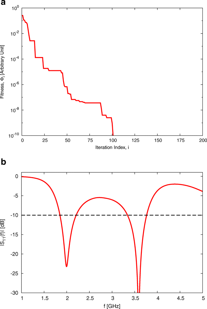
SbD validation (LTE-2100 and LTE-3500 bands). Behavior of Φi vs. the SbD iteration index i (a) and scattering parameter of the optimized layout vs. frequency (b)
For validation purposes, all the s11 plots have been computed by a full-wave MoM-based solver.

Abbreviations
- 3GPP:
-
3rd Generation Partnership Project
- 5G:
-
5th (Fifth) generation
- CPU:
-
Central processing unit
- DoFs:
-
Degrees-of-freedom
- EAs:
-
Evolutionary algorithms
- EM:
-
Electromagnetic
- FCC:
-
Federal Communications Commission
- GPS:
-
Global Positioning System
- GSM:
-
Global System for Mobile Communications
- IoE:
-
Internet of Everything
- IoT:
-
Internet of Things
- LBE:
-
Learning-by-example
- LTE:
-
Long-Term Evolution
- M2M:
-
Machine-to-machine
- MoM:
-
Method-of-Moments
- NFC:
-
Near-field communication
- NB-IoT:
-
Narrowband-IoT
- OA:
-
Orthogonal array
- PC:
-
Personal computer
- POA:
-
Physical objective assessment
- PRE:
-
Physical response emulator
- PS:
-
Particle swarm
- RBF:
-
Radial basis function
- RF:
-
Radio frequency
- RFID:
-
Radio-frequency identification
- SbD:
-
System-by-design
- SSS:
-
Solution-space search
- SVR:
-
Support vector regressor
- UMTS:
-
Universal Mobile Telecommunications System
- WCDMA:
-
Wideband Code Division Multiple Access
- WI-MAX:
-
Worldwide Interoperability for Microwave Access
- WLAN:
-
Wireless local area network
References
M. R. Ebling, Pervasive computing and the Internet of Things. IEEE Pervasive Comput. 15(1), 2–4 (2016).
A. Paraskevopoulos, P. Dallas, K. Siakavara, S. Goudos, Cognitive radio engine design for IoT using real-coded biogeography-based optimization and fuzzy decision making. Wirel. Pers. Commun.97(2), 1813–1833 (2017).
S. Goudos, P. Dallas, S. Chatziefthymiou, S. Kyriazakos, A survey of IoT key enabling and future technologies: 5G, mobile IoT, sematic web and applications. Wirel. Pers. Commun.97(2), 1645–1675 (2017).
Y. Mehmood, C. Gorg, M. Muehleisen, A. Timm-Giel, Mobile M2M communication architectures, upcoming challenges, applications, and future directions. EURASIP J. Wirel. Commun. Netw.2015:, 1–37 (2015).
3GPP, Tr 45.820 Cellular system support for ultra-low complexity and low throughput internet of things (CIoT) (relase 13). Tech. Rep., 1–495 (2015).
3GPP, Ts 36.802, Evolved universal terrestrial radio access (E-UTRA); NB-IoT; technical report for BS and UE radio transmission and reception (release 13). Tech. Rep., 1–59 (2016).
U. Chakraborty, A. Kundu, S. K. Chowdhury, A. K. Bhattacharjee, Compact dual-band microstrip antenna for IEEE 802.11a WLAN application. IEEE Antennas Wirel. Propag. Lett. 13:, 407–410 (2014).
W. Ting, S. Xiao-Wei, L. Ping, B. Hao, Tri-band microstrip-fed monopole antenna with dual-polarisation characteristics for WLAN and WiMAX applications. Electron. Lett.49:, 1597–1598 (2013).
S. K. Mishra, R. K. Gupta, A. Vaidya, J. Mukherjee, A compact dual-band fork-shaped monopole antenna for Bluetooth and UWB applications. IEEE Antennas Wirel. Propag. Lett.10:, 627–630 (2011).
A. Diallo, C. Luxey, P. Le Thuc, R. Staraj, G. Kossiavas, Efficient two-port antenna system for GSM-DCS-UMTS multimode mobile phones. Electron. Lett.43:, 369–370 (2007).
Y. -J. Ren, Ceramic based small LTE MIMO handset antenna. IEEE Trans. Antennas Propag.61(2), 934–938 (2013).
L. Le, V. Lau, E. Jorswieck, N. Dao, A. Haghighat, Kim D., T. Le-Ngoc, Enabling 5G mobile wireless technologies. EURASIP J Wirel. Commun. Netw.2015:, 1–14 (2015).
G. Oliveri, G. Gottardi, F. Robol, A. Polo, L. Poli, M. Salucci, M. Chuan, C. Massagrande, P. Vinetti, M. Mattivi, R. Lombardi, A. Massa, Co-design of unconventional array architectures and antenna elements for 5G base station. IEEE Trans. Antennas Propag.65(12), 6752–6767 (2017).
C. M. Kruesi, R. J. Vyas, M. M. Tentzeris, Design and development of a novel 3-D cubic antenna for wireless sensor networks (WSNs) and RFID applications. IEEE Trans. Antennas Propag. 57(10), 3293–3299 (2009).
Y. Zhou, C. -C. Chen, J. L. Volakis, Single-fed circularly polarized antenna element with reduced coupling for GPS arrays. IEEE Trans. Antennas Propag.56(5), 1469–1472 (2008).
C. Puente-Baliarda, J. Romeu, R. Pous, A. Cardama, On the behavior of the Sierpinski multiband fractal antenna. IEEE Trans. Antennas Propag.46(4), 517–524 (1998).
M. Martinez-Vazquez, O. Litschke, M. Geissler, D. Heberling, A. M. Martinez-Gonzalez, D. Sanchez-Hernandez, Integrated planar multiband antennas for personal communication handsets. IEEE Trans. Antennas Propag.54(2), 384–391 (2006).
E. Zeni, R. Azaro, P. Rocca, A. Massa, Quad-band patch antenna for Galileo and Wi-Max services. Electron. Lett.43:, 960–962 (2007).
R. Azaro, E. Zeni, P. Rocca, A. Massa, Synthesis of a Galileo and Wi-Max three-band fractal-eroded patch antenna. IEEE Antennas Wirel. Propag. Lett.6:, 510–514 (2007).
R. Azaro, F. Viani, L. Lizzi, E. Zeni, A. Massa, A monopolar quad-band antenna based on a Hilbert self-affine pre-fractal geometry. IEEE Antennas Wirel. Propag. Lett.8:, 177–180 (2009).
L. Lizzi, R. Azaro, G. Oliveri, A. Massa, Multiband fractal antenna for wireless communication systems for emergency management. J Electromagn. Waves Applicat.26(1), 1–11 (2012).
F. Viani, M. Salucci, F. Robol, A. Massa, Multiband fractal Zigbee/WLAN antenna for ubiquitous wireless environments. J Electromagn. Waves Appl.26:, 1554–1562 (2012).
F. Viani, M. Salucci, F. Robol, G. Oliveri, A. Massa, Design of a UHF RFID/GPS fractal antenna for logistics management. J Electromagn. Waves Appl.26(4), 480–492 (2012).
E. L. Chuma, Y. Iano, Roger L.L.B., in 2017 SBMO/IEEE MTT-S International Microwave and Optoelectronics Conference (IMOC), Aguas de Lindoia. Compact antenna based on fractal for IoT sub-GHz wireless communications, (2017), pp. 1–5. https://doi.org/10.1109/IMOC.2017.8121016.
D. H. Werner, S. Ganguly, An overview of fractal antenna engineering research. IEEE Antennas Propag. Mag.45(1), 38–57 (2003).
S. R. Best, A discussion on the significance of geometry in determining the resonant behavior of fractal and other non-Euclidean wire antennas. IEEE Antennas Propag. Mag.45(3), 9–28 (2003).
S. R. Best, Operating band comparison of the Perturbated Sierpinski and modified Parany gasket antennas. IEEE Antennas Wirel. Propag. Lett.1:, 35–38 (2002).
R. C. Guido, A note on the practical relationship between filters coefficients and the scaling and wavelets functions of the discrete wavelet transform. Appl. Math. Lett.24(7), 1257–1259 (2011).
R. C. Guido, S. Barbon, L. S. Vieira, F. L Sanchez, C. D Maciel, J. C Pereira, P. R Scalassara, E. S Fonseca, in 2008 IEEE International Symposium on Circuits and Systems, Seattle, WA. Introduction to the Discrete Shapelet Transform and a new paradigm: Joint time-frequency-shape analysis, (2008), pp. 2893–2896. https://doi.org/10.1109/ISCAS.2008.4542062.
E. Guaraglia, Entropy and fractal antennas. Entropy. 18(3), 84 (2016).
E. Guariglia, Harmonic Sierpinski gasket and applications. Entropy. 20(9), 714 (2018).
W. J. Krzysztofik, Fractal geometry in electromagnetics applications - From antenna to metamaterials. Microw. Rev.19(2), 3–14 (2013).
R. G. Hohlfeld, N. L. Cohen, Self-similarity and the geometric requirements for frequency independence in antennae. Fractals. 7(1), 79–84 (1999).
R. Haupt, D. Werner, Genetic algorithms in electromagnetics (Wiley, New Jersey, 2007).
P. Rocca, M. Benedetti, M. Donelli, D. Franceschini, A. Massa, Evolutionary optimization as applied to inverse scattering problems. Inverse Probl.25(12), 1–41 (2009).
P. Rocca, G. Oliveri, A. Massa, Differential evolution as applied to electromagnetics. IEEE Antennas Propag. Mag.53(1), 38–49 (2011).
S. Goudos, C. Kalialakis, R. Mittra, Evolutionary algorithms applied to antennas and propagation: a review of state of the art. Int. J. Antennas Propag.2016:, 1–12 (2016).
G. Oliveri, F. Viani, N. Anselmi, A. Massa, Synthesis of multi-layer WAIM coatings for planar phased arrays within the system-by-design framework. IEEE Trans. Antennas Propag.63(6), 2482–2496 (2015).
G. Oliveri, M. Salucci, N. Anselmi, A. Massa, Multiscale System-by-Design synthesis of printed WAIMs for waveguide array enhancement. IEEE J. Multiscale. Multiphysics Computat. Techn.2:, 84–96 (2017).
G. Oliveri, L. Tenuti, E. Bekele, M. Carlin, A. Massa, An SbD-QCTO approach to the synthesis of isotropic metamaterial lenses. IEEE Antennas Wirel. Propag. Lett.13:, 1783–1786 (2014).
A. Massa, G. Oliveri, M. Salucci, N. Anselmi, P. Rocca, Learning-by-examples techniques as applied to electromagnetics, (2017). https://doi.org/10.1080/09205071.2017.1402713.
A. J. Smola, B. Scholkopf, A tutorial on support vector regression. Stat. Comput.14:, 199–222 (2004).
S. H. Park, Robust design and analysis for quality engineering (Chapman and Hall, London, 1996).
A. S. Hedayat, N. J. A. Sloane, J. Stufken, Orthogonal arrays (Springer, New York, 2013).
Z. Bayraktar, D. H. Werner, P. L. Werner, Miniature meander-line dipole antenna arrays, designed via an orthogonal-array-initialized hybrid particle-swarm optimizer. IEEE Antennas Propagat. Mag.53(3), 42–59 (2011).
C. C. Chang, C. J. Lin, LIBSVM: a library for support vector machines. ACM Trans. Intell. Systems and Tech. 2:, 1–39 (2011).
Y. W. Leung, Y. Wang, An orthogonal genetic algorithm with quantization for global numerical optimization. IEEE Trans. Evolution. Comput.5(1), 41–53 (2001).
N. J. A Sloane, A library of Orthogonal Arrays (2007). http://neilsloane.com/oadir. Accessed 09 Jan 2018.
C. W. Hsu, C. C. Chang, Lin C.J., A practical guide to support vector classification (National Taiwan University, 2003).
Acknowledgments
Not applicable.
Funding
This work benefited from the networking activities carried out within the SNATCH Project (2017–2019) funded by the Italian Ministry of Foreign Affairs and International Cooperation, Directorate General for Cultural and Economic Promotion and Innovation, the Project “WATERTECH - Smart Community per lo Sviluppo e l’Applicazione di Tecnologie di Monitoraggio Innovative per le Reti di Distribuzione Idrica negli usi idropotabili ed agricoli” (Grant no. SCN_00489) funded by the Italian Ministry of Education, University, and Research within the Program “Smart cities and communities and Social Innovation” (CUP: E44G14000060008), and the Project “SMARTOUR - Piattaforma Intelligente per il Turismo” (Grant no. SCN_00166) funded by the Italian Ministry of Education, University, and Research within the Program “Smart cities and communities and Social Innovation”.
Availability of data and materials
Not applicable.
Author information
Authors and Affiliations
Contributions
All authors read and approved the final manuscript.
Corresponding author
Ethics declarations
Competing interests
The authors declare that they have no competing interests.
Publisher’s Note
Springer Nature remains neutral with regard to jurisdictional claims in published maps and institutional affiliations.
Additional information
Authors’ information
Not applicable.
Rights and permissions
Open Access This article is distributed under the terms of the Creative Commons Attribution 4.0 International License (http://creativecommons.org/licenses/by/4.0/), which permits unrestricted use, distribution, and reproduction in any medium, provided you give appropriate credit to the original author(s) and the source, provide a link to the Creative Commons license, and indicate if changes were made.
About this article

Cite this article
Salucci, M., Anselmi, N., Goudos, S. et al. Fast design of multiband fractal antennas through a system-by-design approach for NB-IoT applications. J Wireless Com Network 2019, 68 (2019). https://doi.org/10.1186/s13638-019-1386-4
Received:
Accepted:
Published:
DOI: https://doi.org/10.1186/s13638-019-1386-4