Delay constrained throughput optimization in multi-hop AF relay networks, using limited quantized CSI

Abstract

In this paper, we analyze the throughput of multi-hop amplify and forward (AF) relay networks in delay-constrained scenario. Using quantized channel state information (CSI), the transmission rates and powers are discretely adapted with individual average power constraint on each node. A sub-gradient projection-based algorithm is utilized, by which there is no need for probability density functions (PDFs) to solve the optimization problem. Our numerical evaluations show that the sub-gradient projection-based algorithm results in a comparable performance with an analytical approach using PDFs. As shown, a considerably better performance obtained by the designed scheme compared to previous schemes with constant power transmission. More than 70% throughput improvement is achieved by our scheme compared to constant power transmission with just two more feedback bits and a short training time required at the beginning of the transmission.

1 Introduction

Relaying is a promising tool for expanding the network coverage area and increasing link reliability. Nowadays, there is a great interest in reducing the size of communication tools, thereby reducing power sources and weakening transmitted signals. Thus, when the distance between the transmitter and the receiver is long, multiple relays are deployed in order to have a reliable transmission. Amplify and forward (AF) relaying is less complicated and less costly compared with other relaying schemes, e.g., decode and forward (DF) or compress and forward (CF) relaying [1]. Link adaptation is an efficient tool to overcome multi-path fading effects in wireless channels [2]. In this paper, a new scheme is designed for optimized transmission in a multi-hop AF relay network in which practical constraints for system implementation are considered as follows: (a) Discrete rate adaptation is utilized using adaptive modulation and coding, considering instantaneous block error rate (BLER) constraints. (b) To decrease feedback load, transmitter’s power is selected from a limited discrete set and just the index of the power level is sent back. Discrete rate and power adaptation considerably decrease the sensitivity to imperfect channel state information (CSI). (c) A delay constraint is considered, which makes the proposed scheme suitable for multimedia applications. (d) Independent average power constraint for each relay and the transmitter is considered because in practice nodes have disjoint and independent power supplies. (e) A new version of the proposed scheme is developed which works without any need for the probability density function (PDF) of the signal to interference and noise ratios (SINRs). This satisfies a limitation in practical networks especially mobile systems, where PDFs are not precisely available, e.g., at high speed.

In the following, related principles are illustrated and previous works are reviewed, and then the paper’s contributions and structure are presented.

1.1 Literature survey

1.1.1 Link adaptation, limited feedback, and delay constraint

Link adaptation is an enabling tool to overcome the effect of multi-path fading in wireless channels, by which transmission rate is adapted based on the link’s SINR. There are two approaches to link adaptation, i.e., continuous or discrete. In continuous link adaptation, the transmission rate is continuously adapted based on the channel SINR, and capacity-achieving codes with (asymptotically) zero error probability are used [2]. Continuous link adaptation, though insightful for system performance analysis, is not implementable in practical systems.

In discrete link adaptation, a small BLER is accepted and the transmission rate is chosen from a limited set of discrete rates. There are two approaches to discrete link adaptation in a single carrier link¹: various transmission rates may be obtained by adaptive modulation (AM) [2] or by using adaptive modulation and coding (AMC) [3]. With AM, the instantaneous transmit rate is estimated with a closed-form continuous function; thus, the design of transmission schemes using AM is similar to continuous link adaptation. The performance considerably improves using coding, but the design of transmission schemes with AMC is different and more complicated.

In parallel with rate adaptation, the transmission power may be constant or adapted. For a point to point link, it was shown that continuous power adaptation compared to constant power improves the performance [2]. Note that in a multi-link system, a more complicated strategy may be followed to control instantaneous transmit power taking intra-cell and inter-cell interference into account, e.g., as in the long-term evolution (LTE) standard [4].

With discrete link adaptation and constant transmit power, just the index of the transmission mode is to be sent back. In networks where continuous power adaptation is utilized, channels’ SINRs should be sent to a node at which the optimization problem is solved. Moreover, each node should receive its optimized transmit power. Limited rate control channels are available to exchange the mentioned real numbers; thus, the quantization method is of great importance. Two approaches may be considered for quantization of feedback SINR in a simple power adaptive transmission without automatic repeat request (ARQ): (1) quantizing transmit power based on rate-distortion theory [5] and (2) using discrete levels for power adaptation and sending the index of power level as in [6], where capacity-achieving codes are utilized in a point to point link. However, using ARQ, more efficient quantized feedback may be designed [7, 8].

When using variable transmission rate, generated data may stand in a buffer until it could be transmitted. This causes queuing delay which is to be limited especially in multimedia communication. To this end, delay-constrained throughput is defined in [9]. Provisioning a statistical queuing delay bound for wireless systems in conjunction with link adaptation is investigated in [10–13].

1.1.2 Relay network and utilizing link adaptation

In a relay node, the received signal may be amplified and forwarded (AF relay), or detected, regenerated and forwarded (DF relay), or detected, compressed and forwarded (CF relay). AF relay is less costly and less complicated and has lower forward delay compared to other types. Generally, in an N-hop relay network, the transmitter’s signal passes through N−1 consecutive relays until it is received at the final receiver. If each node only receives the signal of its previous hop, the network is called without diversity, else if it receives signals of different previously placed hops, the network is called with diversity.

The performance of an AF relay network with continuous link adaptation is analyzed in [14–21]. Optimized transmission schemes for an AF relay network using AM are designed in [22–27]. In [14–19] and [22–27], transmission powers are constant or adapted in a way that the sum of the instantaneous powers of the relays and of the transmitter is constrained. In [20] and [21], instead, powers are optimized considering a constraint on the sum of the average transmission powers. Transmission schemes for an AF relay network using AMC and constant transmission power are designed in [28, 29]. In [30, 31], spectral efficiency optimization in a single-hop AF relay network is considered. In [30], spectral efficiency in a single-hop network with diversity is optimized. In [31], the considered network structure is a single-hop relay network with several AF relays between a transmitter and a receiver, and at each time, just one relay is selected to forward the transmitter signal to the receiver.

The paper [32] provides a survey on radio resource management solutions, including link adaptation on orthogonal frequency-division multiple access (OFDMA)-based networks with DF relaying. In [33, 34], optimal power allocation schemes are designed for DF relay network with continues power and rate adaptation. Throughput optimization of DF relay with discrete rate adaptation is addressed in [35–37]. In [38], performance of AF and DF relay networks with continues power and rate adaptation is analyzed.

1.2 Contributions of this work

In this paper, throughput optimized schemes are designed for an N-hop relay network without diversity, to maximize the average spectral efficiency. The list of contributions in this paper is as follows:

• The designed scheme utilizes AMC and power adaptation at all nodes (relays and transmitter), provisioning a detection BLER constraint at the receiver and considering an individual average power constraint for each node. Based on the authors’ knowledge, this is the first work which utilizes discrete rate and power adaptation for a multi-hop AF relay network, especially with practical constraints.

• The presented scheme considers the practical constraints for multimedia communication systems and maximizes delay constrained throughput.

• In general, in a power adaptive transmission scheme, a high CSI load is required, especially in a multi-hop network, SINRs of all hops are to be known at the power adaptive nodes. Moreover, PDFs of SINRs are required to provide average power constraints. Our scheme is designed in such a way that it works with a quite limited CSI load.

  • Each relay adapts its power based on the SINRs of two channels, i.e., the channel towards the next node and that towards the previous node. The mentioned SINRs may be efficiently estimated and monitored at each relay node with good accuracy.

  • Discrete power adaptation is utilized for the main transmitter, in other words, a purpose-driven quantization scheme is designed to adaptively quantize the end-to-end SINR and send the index of appropriate power level. The power levels are agreed upon between the transmitter and the destination at the beginning of the transmission. If Q power levels are considered for each transmission mode, $\log _{2}(Q)$ feedback bits are used to specify the power level.

  • In a modified scheme, the optimization is done using the sub-gradient projection method [39], in which the parameters are set during the transmission through an iterative process without any need to know the PDFs of the random variables involved.

Based on the authors’ knowledge, this is the first work which utilizes the above-mentioned solutions to decrease the CSI load in a discrete rate and power adaptive transmission scheme.

• From the simulation results, it can be inferred that:

  • With continuous power adaptation, considerable better performance is achieved compared to the constant power scheme.

  • With Q=4 discrete power levels for each transmission mode and employing just $\log _{2}(Q)=2$ feedback bits, the performance becomes quite close to that of the continuous power adaptation.

  • As shown using the sub-gradient projection-based method, throughput converges to the value which is obtained by the analytical approach, however, without any need to the SINRs’ PDFs.

1.3 Structure of the paper

The rest of the paper is organized as follows, the network structure, channel model, and other preliminaries are explained in Section 2. In Section 3, a novel scheme is designed to maximize the average spectral efficiency in a multi-hop AF relay network. The designed scheme utilizes AMC and continuous power adaptation at all nodes (relays and transmitter), provisioning a detection BLER constraint at the receiver and considering an individual average power constraint for each node. In Section 4, the presented scheme in Section 3 is modified considering practical constraints (limited CSI load and with delay constraint). In Section 5, as a baseline to evaluate the effect of continuous power adaptation, a transmission scheme using AMC and constant transmission power is analyzed. Section 6 is devoted to the numerical evaluation of the designed schemes and Section 7 concludes the paper.

1.4 Notation

In this paper, scalar variables are denoted by small italic letters, e.g., x, and constants by capital roman letters, e.g., X. The statistical average is denoted by $E\left \{.\right \}$, and [a,b) represents the set of values either greater than or equal to a, and less than b, i.e., a≤x<b. The real part of x is denoted by Real{x}, and the maximum value between x and zero is shown with $\left \lceil x\right \rceil$, i.e., $\left \lceil x\right \rceil =\text {max}(x,0)$. The convolution operation is represented with ∗, the probability function is represented with Prob{}, the secant of x is denoted by sec(x) and exp(x)=e^x.

2 Preliminaries

2.1 System description and channel model

Figure 1 shows the considered N-hop AF relay network without diversity, i.e., the signal of each node is only received at the next node (next relay or the receiver) and does not reach any farther nodes. Nodes from the transmitter to the receiver are labeled with numbers 0 to N, respectively. It is assumed that the transmission power of the i-th node is denoted by p_i, and the channel SINR between the i-th and (i+1)-th nodes is represented by s_i, 0≤i≤N−1. Thus, the received SINR at node N is given by the following equation [40]:

$$ \begin{aligned}\gamma_{eq}=p_{0}s_{eq}=\left(\prod_{i=0}^{N-1}\left(1+\frac{1}{p_{i}s_{i}}\right)-1\right)^{-1}\approx\left(\sum\limits_{i=0}^{N-1}\frac{1}{p_{i}s_{i}}\right)^{-1}\end{aligned}. $$

(1)

Fig. 1

The network structure

We adapt extended pedestrian A (EPA) fading model [41] for channel. In 3GPP standard [42], it is a block fading model in which the channels’ SINRs are fixed during the transmission of each data block from the transmitter to the final receiver.

2.2 Link adaptation method

To analyze the system performance, continuous link adaptation is used by which log₂(1+p₀s_eq) bits/sec/Hz are transmitted where s_eq is the normalized SINR of the equivalent link and p₀ is the transmitter’s power.

In practical systems, discrete link adaptation is implementable, where there are M+1 transmission modes, each implemented by a modulation and a coding scheme that corresponds to a transmission rate R_m, 0≤m≤M, which are sorted as 0=R₀<R₁<R₂⋯_M. The node throughput is μR_m(bits/sec/Hz), where $\mu =\frac {\text {datalength}}{\text {blocklength}}$. AMC is utilized in third generation partnership project (3GPP) LTE with quadrature phase shift keying/quadrature amplitude modulation (QPSK/QAM) and Turbo coding [42], and BLER is approximated as:

$$ p_{e}(\gamma_{eq},\mathrm{R}_{m})=\text{exp}\left\{ \mathrm{A}_{1,m}\text{exp}\left(-\left(\frac{\gamma_{eq}-\mathrm{A}_{2,m}}{\mathrm{A}_{3,m}}\right)^{2}\right)\right\}, $$

(2)

where $\left \{ \mathrm {A}_{1,m},\mathrm {A}_{2,m},\mathrm {A}_{3,m}\right \}$ are mode dependent constants which are derived and listed in Table 1 for the selected set of modes. For the BLER to be less than B₀, it is required that

$$ p_{e}(p_{0}s_{eq},k)\leq B_{0}\Rightarrow p_{0}\geq\frac{g_{B_{0}}(k)}{s_{eq}}, $$

(3)

Table 1 Mode-dependent constants to estimate BLER in LTE standard using (2)

where $k\in \left \{ \mathrm {R}_{0},\cdots,\mathrm {R}_{\mathrm {M}}\right \}$ denotes the instantaneous transmission rate and $g_{B_{0}}(k)$ in LTE is computed as

$$ g_{B_{0}}(k)=\mathrm{A}_{2,m}-\mathrm{A}_{3,m}\sqrt{\ln\left(\frac{\mathrm{A}_{1,m}}{\ln\left(B_{0}\right)}\right)}. $$

(4)

3 Spectral efficiency optimization using AMC and continuous power adaption

This section aims to design a new transmission scheme for maximizing the average spectral efficiency between the transmitter and the receiver in an N-hop relay network. AMC is used at the transmitter and the powers of the transmitter and the relays are continuously adapted. We consider power-constrained users, and to prolong battery life time of energy-saving devices, average transmission power of the i-th node is limited to $\bar {P_{i}},\thinspace 0\leq i\leq N-1$. It is also required that the instantaneous BLER is limited to B₀ at the receiver. The problem of this scheme which is referred to continues adaptive power (CAP) is formulated as:

$$ {\begin{aligned} \max_{p_{i},\thinspace0\leq i\leq N-1}\mu E\left\{ k\right\} =\frac{\mu}{2}\int kf_{s_{0},\cdots,s_{N-1}}(s_{0},\cdots,s_{N-1})ds_{0}\cdots ds_{N-1} \end{aligned}} $$

(5)

subject to:

$$\left\{\begin{array}{ll} C(0),\cdots,C(N-1): & {E\left\{ p_{i}\right\} \leq\bar{P_{i}},0\leq i\leq N-1}\\ C(N): & {{p_{e}\left(\gamma_{eq},k\right){\leq B_{0}}}} \end{array}\right., $$

where $E\left \{ p_{i}\right \} =\frac {1}{2}\int p_{i}f_{s_{0},\cdots,s_{N-1}}(s_{0},\cdots,s_{N-1})ds_{0}\cdots ds_{N-1}$ and $f_{s_{0},\cdots,s_{N-1}}(\ldots)$ is the joint PDF of the random variables s₀,⋯,s_N−1. The problem above is a constrained mixed integer optimization problem, whose solution is not straightforward. A similar problem with continuous link adaptation is solved in Appendix A, and following a similar approach, a solution for (5) is presented. In the following, at first, the powers of all nodes are set and the transmitter’s rate is assigned; next, the problem is reformulated and solved.

As computed in Appendix A, we assign the power of the i-th node, 0≤i≤N−1, as:

$$ p_{i}=q_{i}p_{0};\thinspace q_{i}\triangleq\frac{1}{\alpha_{i}}\sqrt{\frac{s_{0}}{s_{i}}}, $$

(6)

where α₀=q₀=1 and α_i, 1≤i≤N−1 is set in the optimization process. Noting (1), based on the assigned powers, the SINR of the equivalent link between the transmitter and the receiver is derived as:

$$ s_{eq}=\left(\sum\limits_{i=0}^{N-1}\left(\frac{\alpha_{i}}{\sqrt{s_{i}s_{0}}}\right)\right)^{-1}. $$

(7)

To provide the BLER constraint with respect to (3) and to maximize the utilization of the network resource, the transmitter’s power is set as $p_{0}=\frac {g_{B_{0}}(k)}{s_{eq}}$.

To determine the transmission rate, the s_eq axis is divided into M+1 non-overlapping adjacent intervals using the thresholds $0=t_{0}< t_{1}<\cdots < t_{M+1}=\infty$. When s_eq∈[t_m,t_m+1), the transmission rate is set to k=R_m, 1≤m≤M.

According to the assigned powers and rate, the average transmission rate, $E\left \{ k\right \}$, and the average transmission powers of the nodes $E\left \{ p_{i}\right \},\thinspace 0\le i\le N-1$ are respectively computed as:

$$ E\left\{ k\right\} =\frac{1}{2}\sum\limits_{m=0}^{\mathrm{M}}\mathrm{R}_{m}\intop_{t_{m}}^{t_{m+1}}f_{s_{eq}}(s_{eq})ds_{eq}, $$

(8)

$$ \begin{aligned} E\left\{ p_{i}\right\} =&\frac{1}{2}\sum\limits_{m=0}^{\mathrm{M}}g_{B_{0}}(\mathrm{R}_{m})\\&\intop_{t_{m}}^{t_{m+1}}\int_{0}^{\infty}\frac{q_{i}}{s_{eq}}f_{s_{eq},q_{i}}(s_{eq},q_{i})ds_{eq}dq_{i},\thinspace0\le i\le N-1, \end{aligned} $$

where $f_{s_{eq},q_{i}}(.,.)=f_{s_{eq}}(.)$. According to the computed statistical averages, (5) is reformulated as:

$$ \max_{t_{1},\cdots,t_{m}}\mu E\left\{ k\right\} s.t. $$

(9)

$$C(0),\cdots,C(N-1):E\left\{ p_{i}\right\} \le\bar{P_{i}};\thinspace0\le i\le N-1, $$

where constraint C(N) in (5) is now considered in the transmitter’s power assignment. To solve (9), the Lagrangian is set as [43]:

$$ \mathcal{L}=\mu E\left\{ k\right\} -\sum\limits_{i=0}^{N-1}\lambda_{i}\left(E\left\{ p_{i}\right\} -\bar{P_{i}}\right). $$

(10)

Based on Karush-Kuhn-Tucker (KKT) condition [44], As $\frac {\partial ^{2}\mathcal {L}}{\partial t_{m}^{2}}<0$, the Lagrangian is a convex function of t_m and the optimum values of the thresholds are obtained by solving the $\nabla \mathcal {L}=0$ equation as:

$$ \nabla\mathcal{L}=0\Rightarrow t_{m}=\varLambda\frac{g_{B_{0}(\mathrm{R}_{m})}-g_{B_{0}(\mathrm{R}_{m-1})}}{\mathrm{R}_{m}-\mathrm{R}_{m-1}}, $$

(11)

where $\varLambda =\left [\lambda _{0}+{\sum \nolimits }_{i=1}^{N-1}\lambda _{i}\int _{0}^{\infty }f_{q_{i}|s_{eq}}(q_{i}|t_{m})dq_{i}\right ]/\mu$. To finalize the solution, the Lagrangian multipliers λ_i, 0≤i≤N−1 are to be set. Obviously, all power constraints are active, and thus, the Lagrangian multiplies are to be set such that constraints C(0),⋯,C(N−1) in (9) are satisfied with equality [43]. However, finding λ_is is not straightforward. Noting (6) and $\alpha _{i}=\sqrt {\frac {\lambda _{i}}{\lambda _{0}}}$, there is a direct relation between α_i and λ_i; thus, α_i is set to satisfy C(i) with equality, 1≤i≤N−1. Similarly, Λ is set to provide C(0) with equality.

To compute the average powers, $f_{s_{eq},q_{i}}(s_{eq},q_{i}),\thinspace 0\le i\le N-1$ are needed, which are computed in Appendix Appendix B. Computation of $f_{s_{eq}}(.)$ and $f_{s_{eq},q_{i}}(s_{eq},q_{i})$.

4 Throughput optimization by considering practical issues

In this section, practical constraints in the scheme designed in Section 3 are explained and proper solutions are presented to consider them. Finally, (5) is revised to design a modified scheme.

4.1 Practical constraints

4.1.1 Delay constraint

Delay constraint is to be provisioned for multimedia communication systems, while the use of link adaptation with variable transmit rate leads to possible increase of delay due to variable transmission rate and queuing. The delay constrained throughput of a link is formulated in terms of effective capacity in [9, 45, 46] as:

$$ E_{C}(\theta_{0})=\frac{-\thinspace 1}{2\theta_{0}}\log\left(E\left\{ e^{-\theta_{0}\mu k}\right\} \right), $$

(12)

where θ₀ is a parameter related to the delay constraint (the bigger θ₀, the stricter constraint). If the rate of data generation at the source is limited to E_C(θ₀), the queuing delay is exponentially bounded as:

$$ \text{Prob}\left\{ \text{Delay}>T\right\} \le e^{-\theta_{0}T}. $$

(13)

For a given delay constraint, the effective capacity is to be maximized or equivalently $E\left \{ e^{-\theta _{0}\mu k}\right \}$ is to be minimized.

4.1.2 Low-rate feedback channel

Noting to (6), each relay needs to have s₀ to adapt its power which requires a high feedback rate, if real values are to be sent. In this section, we propose solutions to decrease the feedback load.

Noting (6), the formula for the relay’s transmit power can be revised as:

$$ p_{i}=\frac{\alpha_{i-1}}{\alpha_{i}}\sqrt{\frac{s_{i-1}}{s_{i}}}p_{i-1},\thinspace1\le i\le N-1. $$

(14)

Constants α_i−1 and α_i are set at the start of the communication, and SINRs are estimated from the received signal. AF relay-based transmission is usually divided into two phases, including channel estimation through broadcasting of training information and retransmission of information to the destination [47, 48]. In time division duplex (TDD) transmission, the i-th relay can reliably estimate s_i−1 from the training information of (i−1)-th relay and s_i can be acquired through eavesdropping of the training information in channel estimation phase of (i+1)-th relay.

Observing that a discrete set of power levels are assigned to each transmission mode, just index of the power level needs to be sent back to the transmitter. The power levels can be optimized to maximize the overall throughput.

With discrete power adaptation, Q power levels P_m,1,⋯,P_m,Q are used in mode m, 1≤m≤M. The range of s_eq is divided into M+1 coarse intervals which are determined by the thresholds $0=t_{0,1}< t_{1,1}\cdots < t_{M,1}< t_{M+1,1}=\infty$. For s_eq∈[t_m,1,t_m+1,1) the transmission rate is k=R_m. The interval [t_m,1,t_m+1,1) is divided into Q fine consecutive intervals by the thresholds t_m,1<t_m,2⋯<t_m,Q+1=t_m+1,1. It is assumed that when s_eq∈[t_m,n,t_m,n+1), 1≤n≤Q, the transmitter’s power is set as p₀=P_m,n. To satisfy the BLER constraint, the thresholds are set as $P_{m,n}=\frac {g_{B_{0}(\mathrm {R}_{m})}}{t_{m,n}},\thinspace 0\le m\le \mathrm {M},1\le n\le Q$. In this scheme, log₂(M+1)+log₂(Q) feedback bits are required for discrete rate and power adaptation.

4.1.3 Unavailability of PDFs

To complete the solution in Section 3, Lagrange multipliers are found using PDFs. On the other hand, PDFs may not be available in some practical networks, especially in mobile systems. Using sub-gradient projection methods [39], the optimization parameters can be found through an iterative process during transmission without any knowledge of the PDFs. More details are presented in the next subsection.

4.2 Problem reformulation

Given the rate and power assignment strategy developed in the previous section, the effective capacity of the equivalent link and the average powers are computed as:

$$ E_{C}(\theta_{0})=\frac{-\thinspace1}{2\theta_{0}}\log\left[\sum\limits_{m=0}^{\mathrm{M}}e^{-\theta_{0}\mu\mathrm{R}_{m}}\intop_{t_{m,1}}^{t_{m+1,1}}f_{s_{eq}}(s_{eq})ds_{eq}\right], $$

(15)

$$ \begin{aligned} E\left\{ p_{i}\right\} =&\frac{1}{2}\sum\limits_{m=0}^{\mathrm{M}}\sum\limits_{n=1}^{Q}\frac{g_{B_{0}}(\mathrm{R}_{m})}{t_{m,n}}\\&\times\intop_{t_{m,n}}^{t_{m,n+1}}\int_{0}^{\infty}q_{i}f_{s_{eq},q_{i}}(s_{eq},q_{i})ds_{eq}dq_{i},\!\thinspace0\!\le \!i\!\le \!N\,-\,1.\thinspace \end{aligned} $$

(16)

Thus, the throughput optimization problem of this scheme which is referred to discrete adaptive power (DAP) is formulated as:

$$ \min_{\begin{array}{c} t_{m,n};1\le m\le\mathrm{M},1\le n\le Q\end{array}}E\left\{ e^{-\theta_{0}\mu k}\right\} $$

(17)

subject to:

$$C(0),\cdots,C(N-1):E\left\{ p_{i}\right\} \le\bar{P_{i}};\thinspace0\le i\le N-1. $$

4.3 Solution to the modified problem

When PDFs are available, the problem is solved using Lagrange multipliers. The Lagrangian is computed as (10), and thresholds are obtained by solving the equation $\nabla \mathcal {L}=0$ as:

$$ \frac{\partial\mathcal{L}}{\partial t_{m,1}}=0\overset{1\le m\le\mathrm{M}}{\Rightarrow} $$

(18)

$$ \begin{aligned} &\left(-e^{-\theta_{0}\mu\mathrm{R}_{m}}+e^{-\theta_{0}\mu\mathrm{R}_{m-1}}\right)f_{s_{eq}}(t_{m,1})\\&\quad-\sum\limits_{i=0}^{N-1}\frac{\lambda_{i}g_{B_{0}}(\mathrm{R}_{m})}{2\left(t_{m,1}\right)^{2}}\intop_{t_{m,1}}^{t_{m,2}}\int_{0}^{\infty}q_{i}f_{s_{eq},q_{i}}(s_{eq},q_{i})ds_{eq}dq_{i}-\\ &\sum\limits_{i=0}^{N-1}\frac{\lambda_{i}g_{B_{0}}(\mathrm{R}_{m})}{2t_{m,1}}\int_{0}^{\infty}q_{i}f_{s_{eq},q_{i}}(t_{m,1},q_{i})dq_{i}\\&\quad+\sum\limits_{i=0}^{N-1}\frac{\lambda_{i}g_{B_{0}}(\mathrm{R}_{m-1})}{2t_{m-1,Q}}\int_{0}^{\infty}q_{i}f_{s_{eq},q_{i}}(t_{m,1},q_{i})dq_{i}=0, \end{aligned} $$

$$\begin{aligned} &\frac{\partial\mathcal{L}}{\partial t_{m,n}}=0\overset{\begin{array}{c} 1< n<Q\\ 1\le m\le\mathrm{M}\thinspace \end{array}}{\Rightarrow}\sum\limits_{i=0}^{N-1}\frac{\lambda_{i}g_{B_{0}}(\mathrm{R}_{m})}{2\left(t_{m,n}\right)^{2}}\\&\intop_{t_{m,n}}^{t_{m,n+1}}\int_{0}^{\infty}f_{s_{eq},q_{i}}(s_{eq},q_{i})ds_{eq}dq_{i}+\\ &\sum\limits_{i=0}^{N-1}\frac{\lambda_{i}g_{B_{0}}(\mathrm{R}_{m})}{2t_{m,n}}\int_{0}^{\infty}f_{s_{eq},q_{i}}(t_{m,n},q_{i})dq_{i}\\&-\sum\limits_{i=0}^{N-1}\frac{\lambda_{i}g_{B_{0}}(\mathrm{R}_{m})}{2t_{m,n-1}}\int_{0}^{\infty}f_{s_{eq},q_{i}}(t_{m,n},q_{i})dq_{i}=0. \end{aligned} $$

If t_m,n and t_m,n+1 are close to each other, $\intop _{t_{m,n}}^{t_{m,n+1}}\int _{0}^{\infty }f_{s_{eq},q_{i}}(s_{eq},q_{i})ds_{eq}dq_{i}$ can be approximated as $\left (t_{m,n+1}-t_{m,n}\right)\int _{0}^{\infty }f_{s_{eq},q_{i}}(s_{eq},q_{i})ds_{eq}dq_{i}$ and thresholds are approximately obtained as:

$$ \begin{aligned} &\left(-e^{-\theta_{0}\mu\mathrm{R}_{m}}+e^{-\theta_{0}\mu\mathrm{R}_{m-1}}\right)-\left(\frac{t_{m,2}g_{B_{0}}(\mathrm{R}_{m})}{\left(t_{m,1}\right)^{2}}-\frac{g_{B_{0}}(\mathrm{R}_{m-1})}{t_{m-1,Q}}\right)\\&\Lambda=0;\thinspace1\le m\le\mathrm{M}, \end{aligned} $$

(19)

$$\left(t_{m,n}\right)^{2}=t_{m,n-1}t_{m,n+1};\thinspace1\le m\le\mathrm{M},\thinspace1< n\le Q, $$

where $\Lambda =\frac {1}{2}{\sum \nolimits }_{i=0}^{N-1}\lambda _{i}\int _{0}^{\infty }q_{i}f_{s_{eq},q_{i}}(t_{m,1},q_{i})dq_{i}$.

To complete the solution, the Lagrange multipliers are set to satisfy the constraints with equality. They may be computed analytically when the SINR PDFs are available; otherwise, they may be set using sub-gradient projection methods, in which the multipliers are updated using an iterative process as:

$$ \Lambda^{n+1}=\Lambda^{n}+\beta(n)\left\lceil \frac{g_{B_{0}}(k^{n})}{s_{eq}^{n}}-\bar{P_{0}}\right\rceil, $$

(20)

$$ \alpha_{i}^{n+1}=\alpha_{i}^{n}+\beta(n)\left\lceil \frac{1}{\alpha_{i}^{n}}\sqrt{\frac{s_{0}^{n}}{s_{i}^{n}}}\frac{g_{B_{0}}(k^{n})}{s_{eq}^{n}}-\bar{P_{i}}\right\rceil ;\thinspace1\le i<N-1, $$

where $k^{n},s_{eq}^{n}$, and $s_{i}^{n},\thinspace 0\le i\le N-1$ respectively denote the instantaneous transmission rate, the instantaneous SINR of the equivalent link, and the instantaneous SINR of the i-th hop at the n-th transmission block, and Λⁿ and $\alpha _{i}^{n}$ show the values of the Lagrange multipliers at the n-th block.

These multipliers are continuously updated until convergence, i.e., when the difference between the two consecutive multipliers becomes negligible in (20).

The weighting factor, 0<β(n)<1 implements a forgetting factor in the averaging and can be selected to be either asymptotically vanishing or constant. A constant step-size gains robustness to channel non-stationarities, while $\beta (n)\rightarrow 0$ ensures convergence to the average, when the channel is stationary. To optimize between convergence and accuracy for channel non-stationarity, we select β(n)=10⁻⁴. Indeed, β(n) can be vanished as $\frac {1}{n}$ for accommodation to channel stationarity. As a result, β(n) is selected as $\min \left (10^{-4},\frac {1}{n}\right)$ [49].

Steps to compute the thresholds are summarized in the following algorithm.

5 Delay constrained throughput optimization using AMC and constant power

In this section, in order to show the effectiveness of the continuous power adaptation proposed in the previous sections, a baseline scheme is designed for throughput optimized transmission in N-hop relay network with constant powers (CP), where just the index of the transmission rate is sent back to the transmitter and there is no need to know the SINR PDFs. In this scheme, by considering M+1 transmission modes, just log₂(M+1) feedback bits are required for discrete rate adaptation. According to (3), to guarantee the BLER constraint when $\delta =\gamma _{eq}^{-1}\in [1/g_{B_{0}}(\mathrm {R}_{m+1}),1/g_{B_{0}}(\mathrm {R}_{m}))$, the transmission rate is chosen as k=R_m. Thus, the effective capacity is computed as:

$$ C(\theta_{0})=\frac{-\thinspace1}{2\theta_{0}}\log\left[\sum\limits_{m=0}^{\mathrm{M}}e^{-\theta_{0}\mu\mathrm{R}_{m}}\intop_{1/g_{B_{0}}(\mathrm{R}_{m+1})}^{1/g_{B_{0}}(\mathrm{R}_{m})}f_{\delta}(x)dx\right], $$

(21)

where f_δ(.) may be computed using the characteristic function (CHF) of δ. When each link is subject to Nakagami-m fading, i.e., $f_{s_{i}}(x)=\frac {m_{i}^{m}x^{m_{i-1}}}{\left (\bar {p_{i}}\bar {s_{i}}\right)^{m_{i}}\Gamma (m)}\exp \left \{ -\frac {m_{i}x}{\bar {p_{i}}\bar {s_{i}}}\right \}$, the CHF of δ, ψ_δ(.) is computed as [21]:

$$ \psi_{\delta}(w)=\prod_{i=0}^{N-1}\frac{2}{\Gamma(m_{i})}\left(\frac{-\thinspace jwm_{i}}{\bar{p_{i}}\bar{s_{i}}}\right)K_{m_{i}}\left(2\sqrt{\frac{-\thinspace jwm_{i}}{\bar{p_{i}}\bar{s_{i}}}}\right), $$

(22)

where $K_{m_{i}}(.)$ is the Bessel function of type m_i. By using the change of variable w=tan(φ) and noting that $f_{\delta }(x)=\frac {1}{2\pi }\intop _{0}^{\infty }e^{-jwx}\psi _{\delta }(w)dx$, (21) is computed as (23). A similar approach to compute the spectral efficiency in N-hop AF relay network with AM and constant powers was followed in [27].

$$ \begin{aligned} &C(\theta_{0})=\frac{-\thinspace 1}{2\theta_{0}}\log\\&\left(\text{\ensuremath{\sum\limits_{m=0}^{M}}}\frac{\exp\left(-\thinspace \theta_{0}\mu R_{m}\right)}{\pi}\intop_{0}^{\pi/2}\sec^{2}(\varphi)\text{Real}\left\{ \frac{\psi_{\delta}\left(\tan(\varphi)\right)}{j\tan(\varphi)}\right.\right.\\&\left.\left.\left[\exp\left(\frac{-\thinspace j\tan(\varphi)}{g_{B_{0}}(R_{m+1})}\right)-\exp\left(\frac{-\thinspace j\tan(\varphi)}{g_{B_{0}}(R_{m})}\right)\right]\right\}{\vphantom{\intop_{0}^{\pi/2}}} d\varphi\right) \end{aligned} $$

(23)

6 Results and discussions

This section is devoted to the numerical evaluation of the performance of the designed schemes. AMC modes are selected from the LTE standard where the BLER estimation parameters are derived by fitting the simulation curves of BLER versus SINR. The BLER estimation parameters according to (2) are listed in Table 1. The general form of the network structure is depicted in Fig. 1. Several setups are considered to comprehensively evaluate the performance of the designed schemes.

In Fig. 2, a 3-hop network with Rayleigh fading channels is considered. It is assumed that the average SINR of each hops is $\bar {s_{i}}=S_{0}$ and $\bar {P_{i}}=1$ Watt/Hertz (W/Hz), 0≤i≤2. The quality-of-service (QoS) constraints are specified by θ₀=0.05 and B₀=10⁻⁵ (BLER). The achievable effective capacity is depicted for a wide range of average SINRs. A study of these curves leads to the following noticeable observations:

• A considerable performance improvement is seen when continuous or discrete power adaptation is used, compared to the case of constant power transmission.

  Fig. 2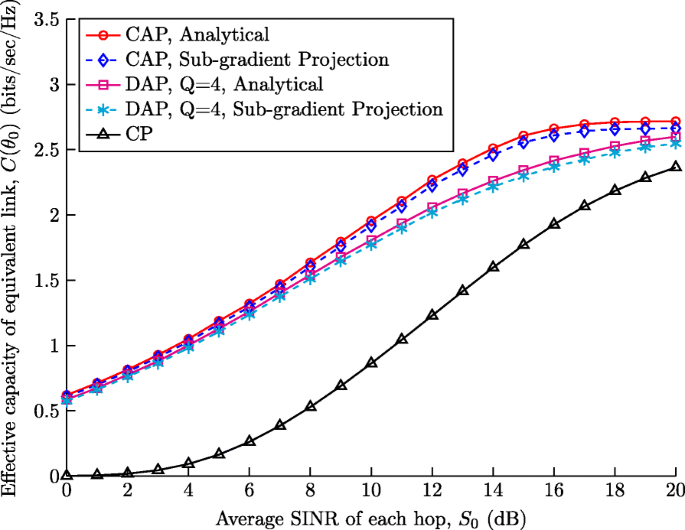

  

  Effective capacity versus average SINR of each hop in different power adaptation schemes, when parameters are obtained analytically or by sub-gradient projection, Rayleigh fading channels $S_{0}=E\left \{ s_{i}\right \}$, $\bar {P_{i}}=1$ W/Hz,  0≤i≤2, B₀=10⁻⁵, θ₀=0.05

• Optimization using the sub-gradient projection method leads to a performance close to the analytical approach; however, the sub-gradient projection method requires considerably less mathematical computations in the design stage and does not need to know the SINR PDFs.

• With discrete power adaptation using Q=4 power levels per mode, the performance is quite close to the performance of continuous power adaptation, while requiring just $\log _{2}(Q)=2$ feedback bits.

In Fig. 3, the effect of increasing the number of relays is investigated while the distance between the transmitter and the receiver is fixed to D₀ and N−1 relays are uniformly placed in the signal’s path. A large-scale path loss model is assumed in which $E\left \{ s_{i}\right \} =\bar {s_{i}}=\frac {K_{0}}{\left (\frac {D_{0}}{N}\right)^{\zeta }}$, where K₀ is a constant and ζ=3 is the path loss exponent. It is assumed that the channels are Nakagami-m fading of order 2. The total sum of the average powers is fixed to P_sum=3 W/Hz, and the average power constraint for each node is $P_{i}=\frac {P_{\text {sum}}}{N},\thinspace 0\le i\le N-1$. The QoS constraints are θ₀=0.1 and B₀=10⁻⁵. The achievable effective capacity is plotted versus N for different transmission power schemes. From the results shown in this figure, the following observations can be made:

• As seen, the overall effective capacity is increased by increasing the number of hops.

  Fig. 3

  

  Effective capacity versus number of relays, when path length is constant, path loss exponent ζ=3, total average power consumption is fixed to 3 W/Hz, B₀=10⁻⁵, θ₀=0.1 and Nakagami-m fading channels with m_i=2, 0≤i≤N−1

• Comparison of the throughputs obtained by different schemes shows that respectively 90% and 80% of the performance gap between the continuous power adaptation and constant power schemes is filled by using just Q=4 (2 bits of feedback) and Q=2 (1 bit) power levels per mode.

By this simulation, we are examining the effect of increasing hardware complexity while the total transmission power is fixed. This numerical evaluation may be employed for a disaster scenario where the infrastructure is lost, and a user in the disaster zone (source) needs multiple relays to get to the nearest active base station. By this simulation, the required number of relays is found and the tradeoff between the number of relays and the power supply of each relay is shown.

In Fig. 4, numerical evaluations are done for responding to an important question in practical systems. The question is that, when the length of the line of sight path between the main transmitter and the final receiver is fixed and the total transmission powers (by the transmitter and relays) is also fixed, does increasing the number of relays (the increase of complexity) leads to improvement in performance or not? We consider three different path loss exponents, ζ=1.8 for special indoor cases, ζ=2 for free space and ζ>2 for most of outdoor cases [50]. As seen, when ζ<2, increasing the number of relays decreases the performance. But when ζ>2, the performance improves by increasing the number of relays.

Fig. 4

Effect of increasing the number of relays, when the length of line of sight path is fixed and total transmission power is fixed for different path loss exponents, ${\sum \nolimits }_{i=0}^{N-1}\bar {P}_{i}=3$ W/Hz, θ₀=0.1

Different behaviors are seen for the path loss exponents lower or more than 2. When ζ>2, the throughput is increasing by increasing the number of relays, while it is decreasing for ζ≤2. To explain this effect, considering (1), γ_eq is the harmonic mean of $\left \{ p_{i}s_{i}\right \}_{i=0}^{N-1}$ divided by N. Noting to the bounds of harmonic mean, we have [51]:

$$ \frac{\min\left\{ p_{i}s_{i}\right\} }{N}\leq\gamma_{eq}<\frac{{\sum\nolimits}_{i=0}^{N-1}p_{i}s_{i}}{N^{2}} $$

(24)

As the considered network is homogeneous, $\frac {E\left \{ p_{i}s_{i}\right \} }{N}$ is a good estimate for $E\left \{ \gamma _{eq}\right \}$. For the ease of computation, we here consider the constant power scheme, and by considering the path loss model, we have:

$$ E\left\{ \gamma_{eq}\right\} \approx\frac{P_{sum}K_{0}}{D_{0}^{\zeta}}N^{\zeta-2} $$

(25)

Obviously, $E\left \{ \gamma _{eq}\right \}$ is increasing by N when ζ>2 and it is decreasing when ζ≤2.

In Fig. 5, the effect of the delay constraint is investigated in a 3-hop network with heterogeneous hops suffering from Nakagami-m fading. It is assumed that $\bar {s_{0}}=2$ dB, m₀=1, $\bar {P_{0}}=1$ W/Hz; $\bar {s_{1}}=3$ dB, m₁=1, $\bar {P_{1}}=1.5$ W/Hz; $\bar {s_{2}}=4$ dB, m₂=2, $\bar {P_{2}}=1$ W/Hz. The required BLER is B₀=10⁻⁵. The achievable effective capacity is plotted versus different values of θ₀, showing the tradeoff in which a more stringent delay constraint (bigger θ₀) results in lower throughput. The QoS exponent, θ₀, may be interpreted as inverse of average and standard deviation of delay. Moreover, the QoS exponent varies between 0.25 and 0.6 in LTE standard [52].

Fig. 5

Effective capacity versus delay constraint, θ₀ in a heterogeneous 3-hop AF relay network; B₀=10⁻⁵, $\bar {s_{0}}=2$ dB, m₀=1, $\bar {P_{0}}=1$ W/Hz; $\bar {s_{1}}=3$ dB, m₁=1, $\bar {P_{1}}=1.5$ W/Hz; $\bar {s_{2}}=4$ dB, m₂=2, $\bar {P_{2}}=1$ W/Hz

Finally, Fig. 6 depicts the convergence behavior of the proposed joint scheduling and link adaptation scheme which utilizes the sub-gradient projection method. A 3-hop network is assumed in which $\bar {s_{i}}=10$ dB, m_i=3, $\bar {P_{i}}=1$ W/Hz,  0≤i≤2;B₀=10⁻⁵, θ₀=0.01, and $\beta =\min \left (10^{-4},\frac {1}{n}\right)$. As seen, a continuous power adaptive scheme using the sub-gradient projection method converges after transmitting an acceptable number of data blocks.

Fig. 6

Effective capacity versus number of transmitted blocks; analytical approach compared with the sub-gradient projection method; $E\left \{ s_{i}\right \} =10$ dB, $\bar {P_{i}}=1$ W/Hz, 0≤i≤2, B₀=10⁻⁵, θ₀=0.01, and Nakagami-m fading channels with m_i=3, 0≤i≤2

7 Conclusion

For an N-hop AF relay network, we have designed a new delay-constrained throughput optimized transmission schemes. Discrete rate adaptation was utilized with adaptive modulation and coding. Discrete power adaptation was utilized, in which a number of power levels were assigned to each transmission mode such that the power levels and their number were adaptively set. A limited quantized feedback is required by discrete rate and power adaptation. A sub-gradient projection-based method was utilized, which does not need knowledge of the SINR PDFs to provide average power constraints. Numerical evaluations show a considerable performance gain obtained by the designed scheme, when compared to constant power transmission. An interesting extension to the proposed scheme is to utilize hybrid ARQ (HARQ) and consider the modified version of the presented scheme in [7]. Another fruitful research direction to extend the current work includes devising link adaptation along with generalized frequency division multiplexing (GFDM) and spectral efficient frequency division multiplexing (SEFDM) to reach the purposes of fifth generation (5G) mobile communication networks.

8 Methods/experimental

The purpose of this study is to analyze the throughput of multi-hop AF relay network in delay constrained and quantized CSI scenario. The system consists of a transmitter node, receiver node, and N−1 AF relay nodes without diversity. The channels between the nodes are assumed to follow Nakagami-m fading. The throughput of the system in terms of effective capacity is optimized using the sub-gradient projection method without any need to know the PDFs of the random variables. Discrete rate and power adaptation are utilized. Discrete rate is utilized with adaptive modulation and coding. Further, a limited number of power levels are assigned to each transmission mode and the power levels are adaptively set.

9 Appendix A. To Solve (5) with continuous rate adaptation

In order to obtain insight on how to solve (5), in this appendix, we consider the same problem with continuous rate adaptation as:

$$ \max_{p_{i};\thinspace0\le i\le N-1}\frac{1}{2}E_{s_{i};\thinspace0\le i\le N-1}\left\{ \log\left[1+\left(\sum\limits_{i=0}^{N-1}\left(p_{i}s_{i}\right)^{-1}\right)^{-1}\right]\right\} $$

(26)

subject to:

$$C(0),\cdots,C(N-1):\frac{1}{2}E_{s_{i};\thinspace0\le i\le N-1}\left\{ p_{i}\right\} \le\bar{P_{i}}. $$

The above problem is a constrained optimization problem, which can be solved via a Lagrangian approach using:

$$ \begin{aligned} \mathcal{L}=&\ E_{s_{i};\thinspace0\le i\le N-1}\left\{ \frac{1}{2}\log\left[1+\left(\sum\limits_{i=0}^{N-1}\left(p_{i}s_{i}\right)^{-1}\right)^{-1}\right]\right\} \\&-\frac{1}{2}\sum\limits_{i=0}^{N-1}\lambda_{i}\left(E\left\{ p_{i}\right\} -\bar{P_{i}}\right). \end{aligned} $$

(27)

As $\frac {\partial ^{2}\mathcal {L}}{\partial p_{i}^{2}}<0$, the Lagrangian is a convex function of p_i, and consequently, the optimum value of p_i is computed by solving $\frac {\partial \mathcal {L}}{\partial p_{i}}=0,\thinspace 0\le i\le N-1$, as [43]:

$$ \begin{aligned} \frac{\partial\mathcal{L}}{\partial p_{i}}=0\Rightarrow\frac{\left({\sum\nolimits}_{i=0}^{N-1}\left(p_{i}s_{i}\right)^{-1}\right)^{-2}s_{i}^{-1}p_{i}^{-2}}{1+\left({\sum\nolimits}_{i=0}^{N-1}\left(p_{i}s_{i}\right)^{-1}\right)^{-1}}=2\lambda_{i}\Rightarrow\\ \left\{\begin{array}{l} p_{i}=\sqrt{\frac{\lambda_{0}}{\lambda_{i}}}\sqrt{\frac{s_{0}}{s_{i}}}p_{0}\\ p_{0}=\frac{s_{eq}}{2\lambda_{0}s_{0}}-\frac{1}{s_{eq}};s_{eq}=\left({\sum\nolimits}_{i=0}^{N-1}\left(\sqrt{\frac{\lambda_{0}}{\lambda_{i}}}\sqrt{s_{0}s_{i}}\right)^{-1}\right)^{-1} \end{array}\right.. \end{aligned} $$

(28)

To complete the solution, the Lagrange multipliers $\left (\lambda _{i},\thinspace 0\le i\le N-1\right)$ are to be determined. As can be seen in (28), if any λ_i is set to zero, i.e., the corresponding power constraint C(i) is ignored, $E\left \{ p_{i}\right \}$ tends to infinity. This means that C(i) is an active constraint, and thus, λ_i is to be set such that $E\left \{ p_{i}\right \} =\bar {P_{i}},\thinspace 0\le i\le N-1$ [43].

10 Appendix B. Computation of $f_{s_{eq}}(.)$ and $f_{s_{eq},q_{i}}(s_{eq},q_{i})$

For ease of computation, instead of s_eq in (7), $r_{eq}=\left (s_{eq}\right)^{-1}$ is considered which may be decomposed as:

$$ {{{r_{eq}=\frac{1}{s_{eq}}=\sum\limits_{i=0}^{N-1}\frac{\alpha_{i}}{\sqrt{s_{0}s_{i}}}={{\frac{1}{s_{0}}+\frac{r_{0}}{\sqrt{s_{0}}};r_{0}=\sum\limits_{i=1}^{N-1}\frac{\alpha_{i}}{\sqrt{s_{i}}}}}}{,}}} $$

(29)

where $f_{r_{eq}}(x)=\int _{0}^{\infty }f_{r_{eq},s_{0}}(x,y)dy$, $f_{r_{eq},s_{0}}(x,y)=f_{s_{0}}(y)f_{r_{eq}|s_{0}}(x|y)$, $f_{r_{eq}|s_{0}}(x|s_{0})=\sqrt {s_{0}}f_{r_{0}}\left (\sqrt {s_{0}}x-\frac {1}{\sqrt {s_{0}}}\right)$ and $f_{r_{0}}(z)$ may be computed using the characteristic function of the random variable $\phantom {\dot {i}\!}r_{0},\psi _{r_{0}}(w)$, as $\phantom {\dot {i}\!}f_{r_{0}}(z)=\frac {1}{2\pi }\intop _{0}^{\infty }e^{-jwz}\psi _{r_{0}}(w)dw$, where $\psi _{r_{0}}(w)=\prod _{i=1}^{N-1}\psi _{i}(w)$ and $\psi _{i}(w)=\intop _{0}^{\infty }\frac {\alpha _{i}}{\sqrt {s_{i}}}f_{s_{i}}(x)e^{jwx}dx$, $f_{s_{i}}(x)=\frac {m_{i}^{m_{i}}x^{m_{i-1}}}{\Gamma (m_{i})\left (\bar {s_{i}}\right)^{m_{i}}}\exp \left \{ -\frac {m_{i}x}{\bar {s_{i}}}\right \},\thinspace 0\le i\le N-1$, when channels suffer from Nakagami-m fading [49].

In a similar way, in order to compute $f_{r_{eq},q_{i}}(.,.)$, r_eq is decomposed as:

$$ r_{eq}=\frac{1}{s_{0}}+\sqrt{\frac{1}{s_{0}}}\underbrace{\left[\sum\limits_{j=1,j\neq i}^{N-1}\frac{\alpha_{j}}{\sqrt{s_{j}}}\right]}_{\acute{r_{0}}}+\frac{1}{q_{i}s_{i}}=\frac{1}{s_{0}}+\frac{1}{\sqrt{s_{0}}}\acute{r_{0}}+\frac{\alpha_{i}^{2}q_{i}}{s_{0}}. $$

(30)

As $f_{r_{eq},q_{i}}(x,y)=\int _{0}^{\infty }f_{r_{eq},q_{i},s_{0}}(x,y,z)dz$ and $f_{r_{eq},q_{i},s_{0}}(x,y,z) =f_{s_{0}}(z)f_{q_{i}|s_{0}}(y|z)f_{r_{eq}|q_{i},s_{0}}(x|y,z)$, we have

$$ f_{q_{i}|s_{0}}(y|z)=\frac{f_{s_{0}}\left(\frac{z}{\alpha_{i}^{2}y^{2}}\right)*(2z)}{\alpha_{i}^{2}y^{3}}, $$

(31)

$$f_{r_{eq}|q_{i},s_{0}}(x|y,z)=\sqrt{z}f_{\acute{r_{0}}}\left(\sqrt{zx}-\left(1+\alpha_{j}^{2}y^{2}\right)/\sqrt{z}\right), $$

where $f_{\acute {r_{0}}}(.)$ is computed similarly to $f_{r_{0}}(.)$.

References

J. N. Laneman, D. N. C. Tse, G. W. Wornell, Cooperative diversity in wireless networks: efficient protocols and outage behavior. IEEE Trans. Inf. Theory. 50(12), 3062–3080 (2004). https://doi.org/10.1109/TIT.2004.838089.
S. T. Chung, A. J. Goldsmith, Degrees of freedom in adaptive modulation: a unified view. IEEE Trans. Commun.49(9), 1561–1571 (2001). https://doi.org/10.1109/26.950343.
K. J. Hole, H. Holm, G. E. Oien, Adaptive multidimensional coded modulation over flat fading channels. IEEE J. Sel. Areas Commun. 18(7), 1153–1158 (2000). https://doi.org/10.1109/49.857915.
M. Bilal, M. Abbas, in Evolved Cellular Network Planning and Optimization for UMTS and LTE. Physical uplink shared channel (PUSCH) closed loop power control for 3G LTE (Auerbach Publications, CRC PressBoca Raton, 2010), pp. 455–486. https://doi.org/10.1201/9781439806500.
K. N. Lau, in IEEE Wireless Communications and Networking (WCNC), vol. 2. Optimal partial feedback design for SISO block fading channels (New Orleans, 2003), pp. 936–940. https://doi.org/10.1109/WCNC.2003.1200497.
A. Gjendemsjø, G. E. Oien, H. Holm, M. -S. Alouini, D. Gesbert, K. J. Hole, P. Orten, Rate and power allocation for discrete-rate link adaptation. EURASIP J. Wirel. Commun. Netw.2008:, 16–11611 (2008). https://doi.org/10.1155/2008/394124.
B. Makki, T. Eriksson, On hybrid ARQ and quantized CSI feedback schemes in quasi-static fading channels. IEEE Trans. Commun.60(4), 986–997 (2012). https://doi.org/10.1109/TCOMM.2012.022912.110324.
B. Makki, T. Eriksson, Feedback subsampling in temporally-correlated slowly-fading channels using quantized CSI. IEEE Trans. Commun.61(6), 2282–2294 (2013). https://doi.org/10.1109/TCOMM.2013.042313.120167.
D. Wu, R. Negi, Effective capacity: a wireless link model for support of quality of service. IEEE Trans. Wirel. Commun.2(4), 630–643 (2003). https://doi.org/10.1109/TWC.2003.814353.
J. Tang, X. Zhang, Quality-of-service driven power and rate adaptation over wireless links. IEEE Trans. Wirel. Commun.6(8), 3058–3068 (2007). https://doi.org/10.1109/TWC.2007.051075.
J. S. Harsini, F. Lahouti, Adaptive transmission policy design for delay-sensitive and bursty packet traffic over wireless fading channels. IEEE Trans. Wirel. Commun.8(2), 776–786 (2009). https://doi.org/10.1109/TWC.2009.071004.
J. Tang, X. Zhang, Cross-layer-model based adaptive resource allocation for statistical QoS guarantees in mobile wireless networks. IEEE Trans. Wirel. Commun.7(6), 2318–2328 (2008). https://doi.org/10.1109/TWC.2008.060293.
J. Xu, X. Shen, J. W. Mark, J. Cai, Adaptive transmission of multi-layered video over wireless fading channels. IEEE Trans. Wirel. Commun.6(6), 2305–2314 (2007). https://doi.org/10.1109/TWC.2007.05838.
M. O. Hasna, M. S. Alouini, Optimal power allocation for relayed transmissions over Rayleigh-fading channels. IEEE Trans. Wirel. Commun.3(6), 1999–2004 (2004). https://doi.org/10.1109/TWC.2004.833447.
Y. Zhao, R. Adve, T. J. Lim, Improving amplify-and-forward relay networks: optimal power allocation versus selection. IEEE Trans. Wirel. Commun.6(8), 3114–3123 (2007). https://doi.org/10.1109/TWC.2007.06026.
K. G. Seddik, A. K. Sadek, W. Su, K. J. R. Liu, Outage analysis and optimal power allocation for multinode relay networks. IEEE Signal Process. Lett.14(6), 377–380 (2007). https://doi.org/10.1109/LSP.2006.888424.
Z. Jingmei, Z. Qi, S. Chunju, W. Ying, Z. Ping, Z. Zhang, in IEEE 59th Vehicular Technology Conference (VTC), vol. 2. Adaptive optimal transmit power allocation for two-hop non-regenerative wireless relaying system (Milan, 2004), pp. 1213–1217. https://doi.org/10.1109/VETECS.2004.1389025.
R. Vaze, R. W. Heath, in IEEE Information Theory Workshop on Networking and Information Theory. Optimal amplify and forward strategy for two-way relay channel with multiple relays (Volos, 2009), pp. 181–185. https://doi.org/10.1109/ITWNIT.2009.5158567.
N. C. Beaulieu, G. Farhadi, Y. Chen, A precise approximation for performance evaluation of amplify-and-forward multihop relaying systems. IEEE Trans. Wirel. Commun.10(12), 3985–3989 (2011). https://doi.org/10.1109/TWC.2011.101811.101133.
G. Farhadi, N. C. Beaulieu, Power-optimized amplify-and-forward multi-hop relaying systems. IEEE Trans. Wirel. Commun.8(9), 4634–4643 (2009). https://doi.org/10.1109/TWC.2009.080987.
G. Farhadi, N. C. Beaulieu, Capacity of amplify-and-forward multi-hop relaying systems under adaptive transmission. IEEE Trans. Commun.58(3), 758–763 (2010). https://doi.org/10.1109/TCOMM.2010.03.080118.
O. Olabiyi, A. Annamalai, in Proceedings of 20th International Conference on Computer Communications and Networks (ICCCN). ASER analysis of cooperative non-regenerative relay systems over generalized fading channels (Maui, 2011), pp. 1–6. https://doi.org/10.1109/ICCCN.2011.6006093.
A. K. Sadek, W. Su, K. J. R. Liu, Multinode cooperative communications in wireless networks. IEEE Trans. Signal Process.55(1), 341–355 (2007). https://doi.org/10.1109/TSP.2006.885773.
C. Qian, Y. Ma, R. Tafazolli, in 7th International Wireless Communications and Mobile Computing Conference. Adaptive modulation for cooperative communications with noisy feedback (Istanbul, 2011), pp. 173–177. https://doi.org/10.1109/IWCMC.2011.5982413.
A. Annamalai, B. Modi, R. Palat, in IEEE Consumer Communications and Networking Conference (CCNC). Analysis of amplify-and-forward cooperative relaying with adaptive modulation in Nakagami-m fading channels (Las Vegas, 2011), pp. 1116–1117. https://doi.org/10.1109/CCNC.2011.5766344.
T. Nechiporenko, K. T. Phan, C. Tellambura, H. H. Nguyen, in IEEE International Conference on Communications. Performance analysis of adaptive M-QAM for Rayleigh fading cooperative systems (Beijing, 2008), pp. 3393–3399. https://doi.org/10.1109/ICC.2008.638.
N. C. Beaulieu, G. Farhadi, Y. Chen, in IEEE Global Telecommunications Conference (GLOBECOM). Amplify-and-forward multihop relaying with adaptive M-QAM in Nakagami-m fading (Kathmandu, 2011), pp. 1–6. https://doi.org/10.1109/GLOCOM.2011.6134065.
B. Modi, O. Olabiyi, A. Annamalai, D. Vaman, in IEEE Global Telecommunications Conference (GLOBECOM). Improving the spectral efficiency of adaptive modulation in amplify-and-forward cooperative relay networks with an adaptive ARQ protocol (Kathmandu, 2011), pp. 1–5. https://doi.org/10.1109/GLOCOM.2011.6134546.
A. Annamalai, B. Modi, O. Olabiyi, in Military Communications Conference (MILCOM). Joint-design of adaptive modulation and coding with adaptive ARQ for cooperative relay networks (Baltimore, 2011), pp. 67–72. https://doi.org/10.1109/MILCOM.2011.6127754.
M. Taki, Spectral efficiency optimisation in amplify and forward relay network with diversity using adaptive rate and adaptive power transmission. IET Commun.7:, 1656–16648 (2013). https://doi.org/10.1049/iet-com.2012.0580.
M. Taki, M. Sadeghi, Joint relay selection and adaption of modulation, coding and transmit power for spectral efficiency optimisation in amplify-forward relay network. IET Commun.8:, 1955–19649 (2014). https://doi.org/10.1049/iet-com.2013.0948.
M. Salem, A. Adinoyi, M. Rahman, H. Yanikomeroglu, D. Falconer, Y. D. Kim, E. Kim, Y. C. Cheong, An overview of radio resource management in relay-enhanced OFDMA-based networks. IEEE Commun. Surv. Tutorials. 12(3), 422–438 (2010). https://doi.org/10.1109/SURV.2010.032210.00071.
X. -X. Nguyen, D. -T. Do, Optimal power allocation and throughput performance of full-duplex DF relaying networks with wireless power transfer-aware channel. EURASIP J. Wirel. Commun. Netw.2017(1), 152 (2017). https://doi.org/10.1186/s13638-017-0936-x.
R. Katla, A. V. Babu, Outage probability analysis and optimal transmit power allocation for multi-hop full duplex relay network over Nakagami-m fading channels. EURASIP J. Wirel. Commun. Netw.2018(1), 192 (2018). https://doi.org/10.1186/s13638-018-1207-1.
N. Yi, Y. Ma, R. Tafazolli, Joint rate adaptation and best-relay selection using limited feedback. IEEE Trans. Wirel. Commun.12(6), 2797–2805 (2013). https://doi.org/10.1109/TWC.2013.050313.120884.
Y. Ma, R. Tafazolli, Y. Zhang, C. Qian, Adaptive modulation for opportunistic decode-and-forward relaying. IEEE Trans. Wirel. Commun.10(7), 2017–2022 (2011). https://doi.org/10.1109/TWC.2011.051311.091773.
K. S. Hwang, M. J. Hossain, Y. C. Ko, M. S. Alouini, in IEEE 20th International Symposium on Personal, Indoor and Mobile Radio Communications. Channel allocation and rate adaptation for relayed transmission over correlated fading channels (Tokyo, 2009), pp. 1477–1481. https://doi.org/10.1109/PIMRC.2009.5450001.
L. Han, B. Shi, W. Zou, Performance analysis and power control for full-duplex relaying with large-scale antenna array at the destination. EURASIP J. Wirel. Commun. Netw.2017(1), 41 (2017). https://doi.org/10.1186/s13638-017-0828-0.
D. P. Bertsekas, Nonlinear Programming, 3rd edn. (Athena Scientific, Nashua, 2016).
M. O. Hasna, M. S. Alouini, Outage probability of multihop transmission over Nakagami fading channels. IEEE Commun. Lett.7(5), 216–218 (2003). https://doi.org/10.1109/LCOMM.2003.812178.
3GPP TS 36.104, LTE; evolved universal terrestrial radio access (E-UTRA); base station (BS) radio transmission and reception. release 8, version 8.2.0 (2008).
3GPP TS 36.212, LTE; evolved universal terrestrial radio access (E-UTRA); multiplexing and channel coding. release 12, version 12.4.0 (2015).
J. Nocedal, S. J. Wright, Numerical Optimization, 2nd edn. (Springer, New York, 2006).
D. G. Luenberger, Y. Ye, Linear and Nonlinear Programming, 3rd edn. (Springer, US, 2008).
D. Wu, R. Negi, Effective capacity-based quality of service measures for wireless networks. Mob. Networks Appl.11(1), 91–99 (2006). https://doi.org/10.1007/s11036-005-4463-3.
J. Jiang, J. Li, R. Hou, X. Liu, Network selection policy based on effective capacity in heterogeneous wireless communication systems. Sci. China Inf. Sci.57(2), 1–7 (2014). https://doi.org/10.1007/s11432-013-4899-1.
F. Gao, T. Cui, A. Nallanathan, On channel estimation and optimal training design for amplify and forward relay networks. IEEE Trans. Wirel. Commun.7(5), 1907–1916 (2008). https://doi.org/10.1109/TWC.2008.070118.
Y. Chen, W. Feng, R. Shi, N. Ge, Pilot-based channel estimation for AF relaying using energy harvesting. IEEE Trans. Veh. Technol.66(8), 6877–6886 (2017). https://doi.org/10.1109/TVT.2017.2654364.
V. Solo, X. Kong, Adaptive Signal Processing Algorithms: Stability and Performance (Prentice-Hall, Inc., Upper Saddle River, 1995).
T. S. Rappaport, Wireless Communications: Principles And Practice, 2nd edn. (Pearson Education, London, 2010).
D. -F. Xia, S. -L. Xu, F. Qi, A proof of the arithmetic mean-geometric mean-harmonic mean inequalities. Technical Report. 2(1) (1999). RGMIA Research Report Collection.
Y. Chen, L. Dong, I. Darwazeh, in 9th International Symposium on Communication Systems, Networks Digital Sign (CSNDSP). Effective capacity-based delay performance estimators for LTE radio bearer QoS provision (Manchester, 2014), pp. 105–110. https://doi.org/10.1109/CSNDSP.2014.6923807.
S. Stiglmayr, M. Bossert, E. Costa, in European Wireless. Adaptive coding and modulation in OFDM systems using BICM and rate-compatible punctured codes (Paris, 2007).
Y. Sui, D. Aronsson, T. Svensson, in Future Network and Mobile Summit. Evaluation of link adaptation methods in multi-user OFDM systems with imperfect channel state information (Warsaw, 2011).
T. Svensson, T. Frank, T. Eriksson, D. Aronsson, M. Sternad, A. Klein, Block interleaved frequency division multiple access for power efficiency, robustness, flexibility, and scalability. EURASIP J. Wirel. Commun. Netw.2009:, 1–18 (2009). https://doi.org/10.1155/2009/720973.
Funding
The authors declare that there is no funding for this work.
Availability of data and materials
Data sharing is not applicable to this article as no datasets were generated or analyzed during the current study.
Author information
Authors and Affiliations
Contributions
The individual contributions of each authors to the manuscript are the same. All authors read and approved the final manuscript.
Corresponding author
Ethics declarations
Competing interests
The authors declare that they have no competing interests.
Publisher’s Note
Springer Nature remains neutral with regard to jurisdictional claims in published maps and institutional affiliations.
Rights and permissions
Open Access This article is distributed under the terms of the Creative Commons Attribution 4.0 International License (http://creativecommons.org/licenses/by/4.0/), which permits unrestricted use, distribution, and reproduction in any medium, provided you give appropriate credit to the original author(s) and the source, provide a link to the Creative Commons license, and indicate if changes were made.
About this article
Cite this article
Taki, M., Svensson, T. & Nezafati, M. Delay constrained throughput optimization in multi-hop AF relay networks, using limited quantized CSI. J Wireless Com Network 2019, 102 (2019). https://doi.org/10.1186/s13638-019-1423-3
Received:
Accepted:
Published:
DOI: https://doi.org/10.1186/s13638-019-1423-3