Improved energy-balanced algorithm for underwater wireless sensor network based on depth threshold and energy level partition

Abstract

Considering the insufficient global energy consumption optimization of the existing routing algorithms for Underwater Wireless Sensor Network (UWSN), a new algorithm, named improved energy-balanced routing (IEBR), is designed in this paper for UWSN. The algorithm includes two stages: routing establishment and data transmission. During the first stage, a mathematical model is constructed for transmission distance to find the neighbors at the optimal distances and the underwater network links are established. In addition, IEBR will select relays based on the depth of the neighbors, minimize the hops in a link based on the depth threshold, and solve the problem of data transmission loop. During the second stage, the links built in the first stage are dynamically changed based on the energy level (EL) differences between the neighboring nodes in the links, so as to achieve energy balance of the entire network and extend the network lifetime significantly. Simulation results show that compared with other typical energy-balanced routing algorithms, IEBR presents superior performance in network lifetime, transmission loss, and data throughput.

1 Introduction

Wireless communication and information technology have been developed to the fifth generation (5G) [1–5], which enabled the realization of various applications based on radio signals [6–10], including satellite systems [11–13], however, they could not be used in an underwater environment. Wireless sensor network (WSN) is wildly used in an underwater environment to collect and transmit data. Underwater WSN (UWSN) can realize wide-area information transmission by underwater sensors, which has certain application value in underwater target detection, underwater Internet of Things construction, marine data collection, disaster prevention, and underwater sonar communication [14]. However, the energy cost by data transmission and the difficulty in battery-replacement in an underwater environment require an efficient and energy-balanced routing protocol to extend the underwater network lifetime. Many existing protocols for UWSN [15–18] might reduce energy consumption, but most of them only consider the problem of local energy consumption.

At present, the energy routing research of UWSN mainly considers consuming energy efficiently. Wahid and Kim [19] proposed a depth-based routing protocol (DBR) by selecting a transponder node based on depth and residual energy, named energy-efficient DBR (EEDBR). Cao et al. [20] studied the balanced transmission mechanism (BTM) for UWSN in the view of energy pattern, in which each node selects a transmission pattern based on its energy level (EL). Li et al. [21] proposed a relative distance-based forwarding (RDBF) protocol. In another work [22], a routing algorithm with efficient energy consumption was proposed based on the sensors’ distance and the residual energy. Mahmood et al. [23] extended DBR and EEDBR, improving the network lifetime. Shen et al. [24] proposed a new energy-efficient centroid-based routing protocol (EECRP) to improve the energy performance of the network, which requires a long lifetime round and base stations located in the network. Azam et al. [25] proposed a balanced load distribution (BLOAD) in order to avoid energy holes caused by energy consumption imbalance, prolonging the stability period and lifetime of UWSN. Javaid et al. [26] proposed two UWSN routing protocols. The first protocol used adaptive hop-by-hop vector-based forwarding (AVN-AHH-VBF) to avoid a void node. The second protocol was cooperation-based AVN-AHH-VBF (CoAVN-AHH-VBF). Ali et al. [27] proposed two protocols: forward layered multipath power control-one (FLMPC-One), and FLMPC Two, reducing the energy consumption and achieving reliability by eluding energy holes. Bengheni et al. [28] proposed an energy management scheme which enhanced energy harvesting. Yousaf et al. [29] proposed a joint rate and power allocation policy (JRPAP), which balanced fairness, throughput, and energy consumption. Yang et al. [30] proposed a hybrid TDMA/CSMA protocol in the MAC layer to improve network energy efficiency and throughput.

For any energy-balanced routing algorithm, the transmitting power of the sensors is the greatest of all working states, which is about 100 times higher than the receiving power [31, 32]. So improving the transmitting energy efficiency is important to improve the data throughput and lifetime of the network. Improved energy-balanced routing (IEBR) adopts the frames of two classical UWSN protocols, BTM and data-aggregating ring (DAR) [33], which will be descripted in Section 2, and it modifies their routing and data transmission mechanisms based on the actual needs of UWSN. IEBR will focus on the global optimaization which can hardly be achieved by the existing energy balance algorithms. Simulation results show that compared with other typical energy-balanced routing algorithms, IEBR processes superior performances in network lifetime, transmission loss, and data throughput.

2 UWSN energy-balanced routing analysis

2.1 BTM and UDAR routing models

The energy balance problem is always an important research field of UWSN. In the routing algorithms for UWSN energy balance, BTM and DAR have good energy balance performance, and their frames are widely adopted to construct the routing models. Figure 1 illustrates the data transmission mechanisms in the models, where the above is BTM and the following is underwater DAR (UDAR).

Fig. 1

Data transmission in BTM and UDAR

BTM is a routing protocol based on hybrid data transmission, which includes two algorithms. Firstly, a tree, whose nodes are sensors and directed edges are links between sensors, is established through efficient routing algorithm (ERA) to determine the transmission route of the data packets, e.g. the multi-hop routes in Fig. 1. Then, the data packets will be transmitted according to the data balanced transmission (DBT) algorithm. BTM divides the initial energy of each node into m ELs. During multi-hop transmission (MT), the closer a sensor to the sink, the more energy it takes to convey the increasing traffic. When the EL of a node decreases from m to m−1, it will broadcast notice packets to all its predecessors. If the EL of the predecessor is higher than that of its successor, the direct transmission (DT) will be adopted to deliver the packets to the sink. For example, in Fig. 1, when EL _B is lower than EL _A, the node A will transmit data to the sink directly. Otherwise, MT will be used, as the multi-hop transmission link from the node A to the sink in Fig. 1. By the way, the transmission pattern can be constantly changed, achieving continuous transmission with balanced energy consumption. However, such mode conversion makes BTM only suitable for small-scale networks, because there are too many direct transmission links in BTM.

UDAR is the derivative model of DAR in underwater environments and it divides all nodes in UWSN into different sets based on the hops to the sink, which is called as hop grade (HG). HG _i is a set of the nodes with hop grade i. HG _i is a circular area in space, which is called as ring sector. As shown in Fig. 1, the nodes in UWSN are divided into HG₁, HG₂, HG₃, and HG₄. The nodes in some HG will collect the data from the nodes in other HGs by MT in a different period and then directly transmit the data to the sink so as to avoid the rapid energy exhaustion of the nodes lying close to the sink. In Fig. 1, the nodes in HG₄ are responsible for collecting data of nodes in other HGs by MT (the green arrows), and then the nodes in HG₄ transmit them to the sink by DT (the blue arrows) along with their own data. It should be noted that the nodes in HG₁ directly transmit data to the sink. UDAR achieves energy balance among different nodes, but it may cause the problem of data transmission loop.

2.2 UWSN energy consumption model

Since the coverage area of the sensor is a circle, given the network radius R, the node density ρ, the maximum number of hops H, and the width of each ring sector w, the total number of nodes can be defined as Eq. (1):

$$\begin{array}{@{}rcl@{}} N=\rho\pi R^{2}=\rho\pi(Hw)^{2} \end{array} $$

(1)

Then, the number of the nodes in HG₁ is shown in Eq. (2). The area of HG₁ is a circle, and the other ring sectors are ring, so they are called as ring sectors. sensors in HG₁, HG _H or other ring sectors have given the network radius R, so they are discussed separately.

$$\begin{array}{@{}rcl@{}} N_{1}=\rho\pi w^{2} \end{array} $$

(2)

Assuming that every node in the UWSN send a data packet at first, according to the different ring sectors, all nodes can be divided into three groups to calculate their energy consumption respectively as follows:(1) The whole energy consumed by nodes in HG₁ is shown as follows:

$$\begin{array}{@{}rcl@{}} E_{1}&=&E_{rx}(\rho\pi H^{2} w^{2}-\rho\pi w^{2})+E_{tx}\rho\pi H^{2}w^{2}\\ &=& \rho\pi w^{2}(E_{rx}(H^{2}-1)+E_{tx}H^{2}) \end{array} $$

(3)

where E_rx and E_txis energy consumption of receiving and transmitting a data packet respectively. The first term in Eq. (3) is the energy consumption of receiving data from nodes in other HGs, and the second term represents the energy consumption of transmitting data to the sink.

(2) The nodes in HG _k (1<k<H) need to receive data from the neighbors in HG _k+1 and send the data along with their own data to the neighbors in HG _k−1. The energy consumption is shown in Eq. (4).

$$\begin{array}{@{}rcl@{}} E_{k}&=& E_{rx}(\rho\pi H^{2}w^{2}\,-\,\rho\pi(kw)^{2})\\ &+&E_{tx}(\rho\pi H^{2}w^{2}\,-\,\rho\pi((k\,-\,1)w)^{2}) \\ &=& \rho\pi w^{2}(E_{rx}(H^{2}-k^{2})+E_{tx}(H^{2}-(k-1)^{2})) \end{array} $$

(4)

(3) The nodes in HG _H only need to send their own data to the nodes in HG _H−1, without accepting data from other nodes. Their energy consumption is shown in Eq. (5).

$$\begin{array}{@{}rcl@{}} E_{H}=\rho\pi w^{2}E_{tx}(H^{2}-(H-1)^{2}) \end{array} $$

(5)

The practical conditions, including the propagation delay and the working frequency range, should also be considered in setting up the underwater energy model [34] to calculate specific energy consumption. The attenuation of the signal with transmission distance d and the frequency f in underwater acoustic channel is defined in Eq. (6).

$$\begin{array}{@{}rcl@{}} A(d,f)=A_{0}d^{k}v^{d} \end{array} $$

(6)

where A₀ is the normalized coefficient, k is the spreading factor, and v is the absorption coefficient, which is based on the signal frequency expressed in kilohertz. The value of k relies on the geometrical shape of the propagation. k is 2 in spherical spreading and is 1 in cylindrical spreading. In addition, v is defined by Eq. (7), where the parameter α is related to the signal frequency f [35]. α can be calculated by Eq. (8) with f exceeding 100 Hz and by Eq. (9) with f lying below. If f is lower, α is shown in Eq. (9). Given f (kHz) and d (km), the transmitting power consumption P_t can be obtained by Eq. (10).

$$\begin{array}{@{}rcl@{}} v=10^{\alpha(f)/10} \end{array} $$

(7)

$$ {}{\begin{aligned} 10\log\alpha(f)=0.002+\frac{0.11f^{2}}{1+f^{2}}+\frac{44f^{2}}{4100+f^{2}}+2.75\times 10^{-4}f^{2}+0.003 \end{aligned}} $$

(8)

$$\begin{array}{@{}rcl@{}} 10\log\alpha(f)=0.002+\frac{0.11f^{2}}{1+f^{2}}+0.011f^{2} \end{array} $$

(9)

$$\begin{array}{@{}rcl@{}} P_{t}=\frac{P_{0}}{A(d,f)} \end{array} $$

(10)

It can be seen from Eq. (10) that factual transmitting power is P_tA(d, f) if the transmitting power is P_t. The transmitting and receiving energy consumption are shown in Eq. (11) and Eq. (12) respectively, where x is the size of transmitted data. r is a constant depending on the receiver.

$$\begin{array}{@{}rcl@{}} E_{tx}(x,d)=P_{t}A(d,f)xt \end{array} $$

(11)

$$\begin{array}{@{}rcl@{}} E_{rx}(x)=rxt \end{array} $$

(12)

3 Improved energy-balanced routing algorithm

Since existing UWSN energy-balanced routing models such as BTM and UDAR have the problem of insufficient global energy balance and transmission loop, IEBR selects the relay nodes according to the distance and depth at the same time, so as to minimize the hops and eliminate the transmission loop in every link. Then, the EL model in BTM will be adopted to establish dynamic links, achieving balanced energy consumption in the same ring sectors and prolonging the network lifetime. In addition, IEBR will also use cross-sector data transmission to achieve energy balance in different ring sectors.

3.1 Network node deployment

Considering the complexity of underwater environments and the inconsistency of the propagating energy consumption, the UWSN topology with ring sector structure in UDAR has been constructed as shown in Fig. 2. The coverage of UWSN is divided into spaced ring sectors Sr₁, Sr₂,…, Sr_n from the inside to the out. Given R, which is the network radius, and O_t, which is the optimal communication distance threshold of sensors, the maximum number of ring sectors is R/O_t. If the transmitting distance exceeds the given O_t, the signal quality will drop sharply to be regarded as unavailable. This threshold has a close corresponding relation with the radius R as shown in Fig. 3. The whole area of UWSN is a concentric circle, where the sink is in the center and other sensors are in the target area randomly and uniformly. Assuming UWSN satisfy the following conditions:

• All sensor nodes have limited battery power

  Fig. 2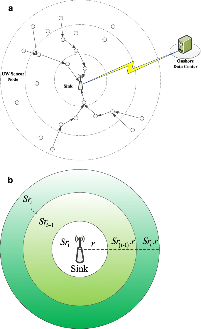

  

  The structure of UWSN. a Network topology. b Ring sector. Sink is on the center to gather data from other nodes and transmits them to data center. All nodes are located in ring sections (Sr) randomly and the radius of each section is r

  Fig. 3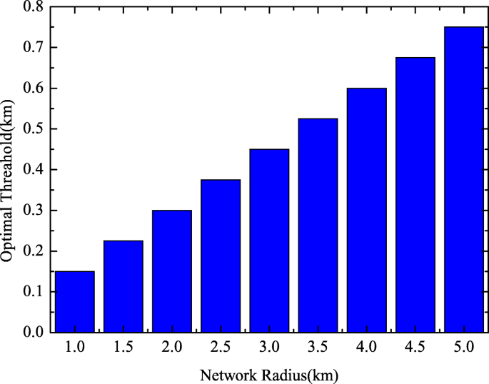

  

  Optimal threshold at different network radiuses. The abscissa is the network radius (km) and the ordinate is the optimal threshold (km)

• The sensor nodes use the positioning methods (received signal strength indication (RSSI) [36] and MoteTrack position recognition scheme [37]) for position sensing in a given underwater environment to make the location known to every sensor

• There are enough data to send for the sensors

• The data reporting mechanism is periodic

• The sink is static and above the water

3.2 Energy-balanced routing (EBR) construction

3.2.1 Relay selection based on optimal distance threshold

After all sensors are deployed as above, if node i not in Sr₁ has data to send, it will select the neighbor at the optimal distance as the relay. Node i will broadcast the location of both itself and the sink s to the neighbors, and every neighbor receiving the data will calculate the parameter N_j according to Eq. (13):

$$\begin{array}{@{}rcl@{}} N_{j}=\alpha|d(i,j)-O_{t}|+(1-\alpha)d(j,s) \end{array} $$

(13)

where d(i, j) is the distance between i and j, α is a system parameter and there is α = 0.5. α gives the same weight to the two distances (distance from node i to relay j and distance from relay j to sink), so the system will consider the effect of two distances on data transmission equally and choose the most appropriate relay based on distance.

The node with the smallest N_j will be the relay, which ensures that the relay node is located at the optimal distance from node i to sink. Figure 4 shows tree typical structures and a list of relays, through which the routing information can be obtained.

Fig. 4

Predecessor and successor with an exemplary relay node table. This is a routing tree, the vertex is the sensor node, the edge is the link between the nodes. The table below shows information about relay nodes

When a relay j is obtained, the parameter N_j will be stored in the routing table of its predecessor i. Then j will inform its successor the fact of j’s being selected as the relay and the node number in the routing table along with N_j. To reduce the node power consumption, the algorithm will allow each node forwarding packets from at most two neighbors.

The process of selecting a relay node with N_j is shown in Fig. 5. Firstly, node i identifies all its neighbors by sending query packets, such as the neighbors q, k, and m in Fig. 5. Then node i will select a relay from its neighbors based on N_j. The algorithm will calculate the distance between node i and its neighbor (black arrow) and the distance between the neighbor and the sink (blue arrow). In Fig. 5, node i selects neighbor j as the relay. After that, the node j will select its relay x. This process will continue until a complete link from i to the sink has been established. The specific routing algorithm can be seen in Table 1.

Fig. 5

Selection of relay nodes with N_j. Source node calculates the distance between and the neighbor; obtains the distance between the neighbor node and sink from the neighbor node, calculating N_j of all neighbors; and selects the relay node

Table 1 Routing establishment of EBR

3.2.2 Data transmission mode based on EL consumption

EBR may get a set of nodes based on the value of N_j and establish a link from node i to the sink among these nodes to transmit data. The initial energy E₀ of each node is divided into L ELs, the Unit EL (UEL) is defined as Eq. (14).

$$\begin{array}{@{}rcl@{}} UEL=\frac{E_{0}}{L} \end{array} $$

(14)

The energy consumption of nodes i and j is calculated by Eq. (15), including the energy consumption of sensing, receiving, and transmitting. x is the data size and d is the transmitting distance.

$$\begin{array}{@{}rcl@{}} E_{t}^{i,j}(x,d)=E_{sen}^{i}(x)+E_{rx}^{j}(x)+E_{tx}^{i}(x,d) \end{array} $$

(15)

During the data transmission, all the sensors in different ring sectors have the same initial ELs. If there is UEL= β, EL of node j in Sr_i and node k in Sr_i−1 are shown in Eqs. (16) and (17), respectively.

$$\begin{array}{@{}rcl@{}} E_{EL}^{j}=\frac{E_{0}}{\beta} \end{array} $$

(16)

$$\begin{array}{@{}rcl@{}} E_{EL}^{k}=\frac{E_{0}}{\beta} \end{array} $$

(17)

As shown in Fig. 6, two conditions may occur during data transmission. In the right link, the EL of each node is equal to that of the successor, so the entire link topology remains the same. In the left link, the transmission load of i and j are different for they are located in different ring sections resulting in EL _j< EL _i. Then, node j will send a control packet to node i, and the link between them is cut off. Now, node j will only transmit its own data along the original link, and node i will have to build a new one. Each relay in the new link is the node with maximum EL in the neighbors. This operation can balance the energy consumption of all sensors in the same ring sectors. Related algorithms are shown in Table 2.

Fig. 6

Data transmission based on EL difference. The link between nodes are dynamic, if EL of successor is lower, the node will find a new relay, and a link become two links by this way

Table 2 Data transmission of EBR

3.3 Realization of improved EBR (IEBR)

3.3.1 Relay node selection model based on depth

To solve the problem of transmission loop, IEBR will take the depth threshold to limit the neighbor number, and the depth of a node depends on the ring sector where the node is located. The nodes in the same ring sector have the same depth. The closer a node lies to the sink, the smaller depth a node will have. A node will get the depth of its neighbors by broadcasting control packets when it has data to transmit. The sensor node will select the neighbors with smaller depth as the relay candidates. After that, the algorithm will select only one node with smallest N_j from all candidates as the relay. The data transmission of IEBR is also based on EL. A sensor will not reselect the relay until the EL of its successor falls below that of itself.

The sensor with greater depth will not be selected as the relay according to IEBR; however, traditional BTM and EBR leave the depth of the node out of account, resulting in the transmission loop, as A→B→A in Fig. 7, so the data packets cannot be transmitted to the sink or additional hops are required, as A→B→C in Fig. 7, which will increase the energy consumption and cause lifetime reduction. For the special condition with no neighbor or only one neighbor B existing, the sensor A will expand the communication range to contain more neighbors [38] so as to establish IEBR loop-free transmission. The routing establishment process of IEBR is shown in Table 3.

Fig. 7

Routing problems during data transmissions. Formation of loops during data transmissions without using depth of the neighbors

Table 3 Routing establishment of IEBR

3.3.2 Cross-sector data transmission

To reduce the hops and the transmission loads, IEBR will search for the relays in every other ring sectors instead of in adjacent ring sectors, i.e., a node in Sr_i will look for the relay node in Sr_i−2 instead of Sr_i−1.

Suppose that there are four nodes A∈ Sr₁, B∈Sr₂, C∈Sr₃, and D∈Sr₄. A and B send data to C and D, respectively. The same volume of data being transmitted at the same distance will have the same energy consumption. C receives the data from A and will send the data as well as its own data, the UEL of C will drop faster than A, which will make A reselect the relay node. Then node C will head to send its own data, node A will begin to send data to another node with a higher EL and the data load is shared by different nodes in this way. Finally, the energy consumption of all ring sectors can achieve balance.

Moreover, the node number in every ring sector is assumed to be the same fixed value in the mathematical mode for simplifying the calculation. In IEBR, it will vary according to the data load as well as the distance to the sink, and the nodes in a ring sector with higher energy consumption will be more, prolonging the lifetime of UWSN for longer lifetimes of these ring sectors.

3.3.3 Packet loss rate constraint of IEBR algorithm

The energy balance algorithm in UWSN will always cause packets lost increasingly so as to limit the practical application. Thus, a maximum throughput model is established in IEBR to reduce the packet loss rate along while achieving global energy balance. Linear programming is used in the paper to design the objective function $\text {Maximize}\sum _{t=1}^{t_{\text {max}}}T_{p}(r)$, and it should satisfy the following constraints:

(i) E_u≤E₀, ∀u∈N;

(ii) d_{u, v}≤d_opt, ∀u, v∈N;

(iii) f_{u, v}≤f_max, ∀u, v∈N;

(iv) d_min≤d_u≤d_max;

(v) P_l≥P_g, ∀u∈N;

(vi) $\sum _{u=1}^{n}E(u)\cong \sum _{v=1}^{m}E(v), \quad \forall u,v\in N$;

The objective function will maximize the number of effective packets received by the sink during time t_max. (i) is the energy constraint, and each sensor u’s energy is E₀ at first. All sensors’ energy should be consumed efficiently to extend the network lifetime and increase throughput. (ii) requires that the distance between two communication nodes u and v not exceed the optimal transmission distance d_opt to keep the packet loss rate from increasing. (iii) describes the constraint of data flow in physical link. f_max is the upper limit of data flow, and it can be defined as the maximum number of packets that can be transmitted per unit time when the size of each packet is fixed. The data flow from any node u to another node v should be less than f_max to ensure that packet loss rate is acceptable. (iv) indicates the upper limit and lower limit of the transmission distance, d_max and d_min. Transmitting data over a long distance by expanding the transmission range will result in a large amount of packets loss while reducing the transmission range will cause higher energy consumption, shorter network lifetime, and higher packet loss rate. IEBR is a reasonable trade-off in the view of the global performance. (v) indicates that the probability P_l of the current link state should be no less than P_g, which is the minimum probability required for successful data transmission [39]. (vi) indicates that the energy consumption of every ring sector should be approximately equal. If the energy consumption is balanced, the network can achieve high throughput so as to prolong the effective lifetime.

4 Performance evaluation

The performance of the proposed IEBR will be verified by cross comparison with BTM and UDAR. In addition, EBR will be adopted as an independent algorithm to evaluate the impact of various elements and stages of the algorithm model.

For EBR, BTM, and UDAR, there are the same number of sensors lying in each ring sector of UWSN in the simulation. The initial energy of each sensor node is 300 J, and the transmission data packet size is 200 bits: 50 bits in the control field, 150 bits in the data field. Carrier sense multiple access with collision avoidance (CSMA/CA) is adopted under IEEE 802.15.4. IEBR model uses Linprog linear programming to achieve the throughput optimization. Network lifetime, effective throughput and transmission loss are used to evaluate the network performance. Network lifetime defined by BTM is evaluated by the maximum transmission rounds (r) that can be achieved. Effective throughput is the number of valid packets (p) received by the sink successfully. Some parameters are shown in Table 4.

Table 4 Simulation parameters

4.1 Network lifetime with different network radiuses

The network lifetime comparison of the algorithms on different network scales is shown in Fig. 8. The curves show that the network lifetime of all algorithms will decrease with the increase of the network radius. When the radius is less than 2 km, the network lifetime falls obviously, but the decline curves of IEBR and EBR are an obvious flat to achieve better lifetime performance. Specifically, the network lifetime of IEBR is about 1.5 times and twice more than that of BTM and UDAR, respectively. When the radius of the network exceeds 3 km, the falling trend of the network lifetime tends to be flat. The network lifetime of IEBR is still higher than the other algorithms, about 1.5 times higher than EBR, and about twice higher than UDAR and BTM. Overall, IEBR performs better in the network lifetime on different network scales, which is mainly because IEBR is able to reduce the hops as well as the data load of the sensors near the sink.

Fig. 8

The network lifetimes with different network radiuses

4.2 Transmission loss with different network radiuses

The transmission loss caused by the balanced algorithms with different network sizes is shown in Fig. 9, which indicates that the transmission loss will increase with the network radius for all algorithms. The increasing trend of IEBR, however, is relatively flat. The transmission loss curves are roughly the same when the network radius is 1km. With the network radius increasing by every 1km, the transmission loss of IEBR and EBR will increase by about 5 dB and 7 dB, respectively, while that of BTM and UDAR will exceed 10 dB and 12 dB, respectively. The advantage of the IEBR algorithm is relatively obvious. When the network radius reaches 5 km, the transmission loss of UDAR is about 30 dB higher than IEBR, the increment is 20 dB for BTM, and is about 10 dB for EBR. It can be seen that IEBR will cause low transmission loss while processing a long network lifetime.

Fig. 9

The transmission loss with different network radiuses

4.3 Effective throughput with different network radiuses

Considering the multi-hop forwarding characteristics of UWSN, the number of effective data packets received is used as the measure of throughput. The effective throughput comparison with different network radiuses is shown in Fig. 10. The effective throughput will decline with the network radius increasing. That is because the increase in the network radius will cause the decrease in node density with constant node number. And the increase in distance between two neighbors will cause the packet loss rate to increase. Specifically, when the radius is 1 km, the effective throughput of IEBR is approximately 8 times more than that of UDAR. After that, the effective throughput will drop sharply with the radius increasing, but it is still higher than that of the other algorithms. That means IEBR has an advantage in effective throughput, especially in the network with the limited radius, which is similar with the simulation results in network lifetime.

Fig. 10

The effective throughput with different network radiuses

4.4 Network lifetime with different network radiuses and node numbers

In the previous simulation, the node number is a constant. The increase in the radius means the decrease in the node density. The comparison of network lifetime in different sizes and scales is shown in Fig. 11. There is a similar trend in the simulating lifetime curves of all balanced algorithms with the node number increasing from 80 to 160. The maximum network lifetime occurs when the number is about 120 and the network radius is 1 km, which is related to the construction of the network model. When the network radius increases to 3 km, IEBR shows a great sensitivity to the node number. When it increases (or decreases) by 10, the network lifetime will increase (or decrease) by about 200. With the node increasing from 80 to 120 in the simulation, IEBR will prolong the network lifetime by about 25%. The comparisons show that IEBR has an advantage in network lifetime over other algorithms with different network radiuses and numbers of nodes.

Fig. 11

The network lifetimes with different network radiuses and numbers of nodes. a Network radius = 1 km. b Network radius = 2 km. c Network radius = 3 km. d Network radius = 4 km. e Network radius = 5 km

4.5 Effective throughput with different network radiuses and node numbers

The comparison of the effective throughput with different network radiuses and numbers of nodes are shown in Fig. 12. The effective throughput is less sensitive to the node density when the network radius is small. With the radius increasing, the effective throughput of the network will rise first and then gradually decline, which is similar to the lifetime curves. When the node number is about 120, the values of effective throughput are the largest with different network radiuses. The larger lifetime means more data transmission and reception, and the effective throughput could be larger, which is similar to the results in Fig. 11. Under different node density conditions, IEBR will have high effective throughput and relatively stable performance in a small-scale network.

Fig. 12

The effective throughput with different network radiuses and numbers of nodes. a Network radius = 1 km. b Network radius = 2 km. c Network radius = 3 km. d Network radius = 4 km. e Network radius = 5 km

5 Conclusion

To solve the problem of limited energy and short lifetime in UWSN, an improved energy balance routing (IEBR) algorithm is presented in this paper. A ring sector model is constructed, and the optimal relay node is selected by transmission distance and depth threshold to avoid the transmission loop. IEBR will select the optimal relay node among different ring sectors alternately, and the link structure will be adjusted dynamically according to the energy level difference. Simulation results show that IEBR has a longer network lifetime, larger effective throughput, and lower transmission loss than the existing typical algorithms in UWSN with different sizes and scales. Moreover, the research indicates that IEBR achieves global energy balance rather than the local balance as the existing algorithms do. Futural research will consider the spatial expansion of the energy ring sectors and the model of dynamic depth thresholds.

References

L Xin, J Min, Z Xueyan, et al., A novel multi-channel Internet of Things based on dynamic spectrum sharing in 5G communication[J]. IEEE Internet of Things J.6:, 1–1 (2018).
X Liu, F Li, Z Na, Optimal resource allocation in simultaneous cooperative spectrum sensing and energy harvesting for multichannel cognitive radio[J]. IEEE Access. 5:, 1–1 (2017).
X Liu, M Jia, Z Na, et al., Multi-modal cooperative spectrum sensing based on Dempster-Shafer fusion in 5G-based cognitive radio[J]. IEEE Access. 6(99), 199–208 (2018).
Z Na, Y Wang, X Li, et al., Subcarrier allocation based simultaneous wireless information and power transfer algorithm in 5G cooperative OFDM communication systems[J]. Phys. Commun.29:, 164–170 (2018).
Z Na, J Lv, M Zhang, et al., GFDM based wireless powered communication for cooperative relay system[J]. IEEE Access. 7:, 50971–50979 (2019).
MA Shaolin, Y Wang, Design and implementation of an ultra-wideband high-accuracy ranging system[J]. J. Tianjin Norm. Univ.(Nat. Sci. Ed.)37(6), 55–57 (2017).
X Zhang, Z Zhang, Near-field plate applied in wireless power transmission system[J]. J. Tianjin Norm. Univ. (Nat. Sci. Ed.)37(6), 58–61 (2017).
J Wu, C Zeng, J Sun, Research and application of wireless intelligent network monitoring smog system based on STM32F407[J]. J. Tianjin Norm. Univ. (Nat. Sci. Ed.)37(6), 62–66 (2017).
Z Liu, J Chen, Y Tong, F Duan, JI Maolin, Research and implementation of digital baseband signal transmission[J]. J. Tianjin Norm. Univ. (Nat. Sci. Ed.)38(1), 51–55 (2018).
B Liang, J Xie, J Shi, W Wang, Design and implementation of three-phase inverter for microgrid research[J]. J. Tianjin Norm. Univ. (Nat. Sci. Ed.)38(1), 59–63 (2018).
M Jia, X Gu, Q Guo, W Xiang, N Zhang, Broadband hybrid satellite-terrestrial communication systems based on cognitive radio toward 5G. IEEE Wirel. Commun.23(6), 96–106 (2016).
M Jia, X Liu, X Gu, Q Guo, Joint cooperative spectrum sensing and channel selection optimization for satellite communication systems based on cognitive radio. Int. J. Satell. Commun. Netw.35(2), 139–150 (2017).
M Jia, X Liu, Z Yin, Q Guo, X Gu, Joint cooperative spectrum sensing and spectrum opportunity for satellite cluster communication networks. Ad Hoc Netw.58(C), 231–238 (2016).
IF Akyildiz, D Pompili, T Melodia, Underwater acoustic sensor networks: research challenges[J]. Ad Hoc Netw.3(3), 257–279 (2005).
NZ Zenia, MS Kaiser, MR Ahmed, et al., in Electrical Engineering and Information Communication Technology (ICEEICT), 2015 International Conference on. An energy efficient and reliable cluster-based adaptive mac protocol for uwsn[C] (IEEEDhaka, 2015), pp. 1–7.
A Solayappan, MBH Frej, SN Rajan, in Systems, Applications and Technology Conference (LISAT), 2017 IEEE Long Island. Energy efficient routing protocols and efficient bandwidth techniques in Underwater Wireless Sensor Networks-a survey[C] (IEEEFarmingdale, 2017), pp. 1–7.
Z Wan, S Liu, W Ni, et al., An energy-efficient multi-level adaptive clustering routing algorithm for underwater wireless sensor networks[J]. Clust Comput, 1–10 (2018).
S Souiki, M Hadjila, M Feham, in Programming and Systems (ISPS), 2015 12th International Symposium on. Energy efficient routing for,obile underwater wireless sensor networks[C] (IEEEAlgiers, 2015), pp. 1–6.
A Wahid, D Kim, An energy efficient localization-free routing protocol for underwater wireless sensor networks[J]. Int. J. Distrib. Sensor Netw.8(4), 307246 (2012).
J Cao, J Dou, S Dong, Balance transmission mechanism in underwater acoustic sensor networks[J]. Int. J. Distrib. Sensor Netw.11(3), 429340 (2015).
ZL Li, NM Yao, Q Gao, Relative distance-based forwarding protocol for underwater wireless sensor networks[C]. Trans. Tech. Publ. Appl. Mech. Mater.437:, 655–658 (2013).
A Wahid, S Lee, D Kim, in 2011 IEEE-Spain OCEANS. An energy-efficient routing protocol for UWSNs using physical distance and residual energy[C] (IEEESantander, 2011), pp. 1–6.
S Mahmood, H Nasir, S Tariq, et al., Forwarding nodes constraint based DBR (CDBR) and EEDBR (CEEDBR) in underwater WSNs[J]. Procedia Comput. Sci.34:, 228–235 (2014).
J Shen, A Wang, C Wang, et al., An efficient centroid-based routing protocol for energy management in WSN-assisted IoT[J]. IEEE Access. 5:, 9–18479 (1846).
I Azam, N Javaid, A Ahmad, et al., Balanced load distribution with energy hole avoidance in underwater WSNs[J]. IEEE Access. 5:, 15206–15221 (2017).
N Javaid, T Hafeez, Z Wadud, et al., Establishing a cooperation-based and void node avoiding energy-efficient underwater WSN for a Cloud[J]. IEEE Access. 5:, 11582–11593 (2017).
B Ali, N Javaid, AR Hameed, et al., in Wireless Communications and Mobile Computing Conference (IWCMC), 2017 13th International. Energy hole avoidance based routing for underwater WSNs[C] (IEEEValencia, 2017), pp. 1654–1659.
A Bengheni, F Didi, I Bambrik, EEM-EHWSN: Enhanced energy management scheme in energy harvesting wireless sensor networks[J]. Wirel. Netw.25(6), 3029–3046 (2019).
R Yousaf, R Ahmad, W Ahmed, et al., A unified approach of energy and data cooperation in energy harvesting WSNs[J]. Sci. China Inf. Sci.61(8), 082303 (2018).
X Yang, L Wang, J Xie, et al., Energy efficiency TDMA/CSMA hybrid protocol with power control for WSN[J]. Wirel. Commun. Mob. Comput.2018: (2018).
III Harris AF, M Stojanovic, M Zorzi, in Proceedings of the 1st ACM international workshop on Underwater networks. When underwater acoustic nodes should sleep with one eye open: idle-time power management in underwater sensor networks[C] (ACMLos Angeles, 2006), pp. 105–108.
AA Syed, W Ye, J Heidemann, in The 27th Conference on Computer Communications. IEEE. INFOCOM 2008. T-Lohi: A new class of MAC protocols for underwater acoustic sensor networks[C] (IEEEPhoenix, 2008), pp. 231–235.
Y Bi, N Li, L Sun, DAR: An energy-balanced data-gathering scheme for wireless sensor networks[J]. Comput. Commun.30(14-15), 2812–2825 (2007).
J Poncela, MC Aguayo, P Otero, Wireless underwater communications[J]. Wirel. Pers. Commun.64(3), 547–560 (2012).
M Stojanovic, On the relationship between capacity and distance in an underwater acoustic communication channel[J]. ACM SIGMOBILE Mob. Comput. Commun. Rev.11(4), 34–43 (2007).
KM Kwak, J Kim, Development of 3-dimensional sensor nodes using electro-magnetic waves for underwater localization[J]. J. Inst. Control Robot. Syst.19(2), 107–112 (2013).
K Lorincz, M Welsh, in International Symposium on Location-and Context-Awareness. Motetrack: A robust, decentralized approach to rf-based location tracking[C] (SpringerBerlin, 2005), pp. 63–82.
M Zorzi, P Casari, N Baldo, et al., Energy-efficient routing schemes for underwater acoustic networks[J]. IEEE J. Sel. Areas Commun.26(9), 1754–1766 (2008).
A Ahmad, N Javaid, ZA Khan, et al., (A C H)2: Routing Scheme to Maximize Lifetime and Throughput of Wireless Sensor Networks[J]. IEEE Sensors J.14(10), 3516–3532 (2014).
Funding
The funding was supported by the National High Technology Research and Development Program of China (2012AA120802),National Natural Science Foundation of China (61771186), Postdoctoral Research of Heilongjiang Province (LBH-Q15121), and Undergraduate University Project of Young Scientist Creative Talent of Heilongjiang Province (UNPYSCT-2017125).
Author information
Authors and Affiliations
Contributions
PF and DyQ conceptualized the idea and designed the experiments. PF contributed in writing and draft preparation and DyQ supervised the research. All authors read and approved the final manuscript.
Corresponding author
Ethics declarations
Competing interests
The authors declare that they have no competing interests.
Additional information
Publisher’s Note
Springer Nature remains neutral with regard to jurisdictional claims in published maps and institutional affiliations.
Rights and permissions
Open Access This article is distributed under the terms of the Creative Commons Attribution 4.0 International License(http://creativecommons.org/licenses/by/4.0/), which permits unrestricted use, distribution, and reproduction in any medium, provided you give appropriate credit to the original author(s) and the source, provide a link to the Creative Commons license, and indicate if changes were made.
About this article
Cite this article
Feng, P., Qin, D., Ji, P. et al. Improved energy-balanced algorithm for underwater wireless sensor network based on depth threshold and energy level partition. J Wireless Com Network 2019, 228 (2019). https://doi.org/10.1186/s13638-019-1533-y
Received:
Accepted:
Published:
DOI: https://doi.org/10.1186/s13638-019-1533-y