On the coexistence of broadcast and unicast in hybrid networks for the transmission of video services using stochastic geometry

Abstract

Following the increasing growth in the demand on mobile TV, hybrid broadcast/broadband networks emerged as a suitable approach to overtake the challenges introduced by each network separately in order to enhance users’ experience. This paper presents two possible scenarios for a hybrid, spatially separated, broadcast/broadband network to offer mobile TV linear services for the end users. Namely, the first scenario is based on shared spectrum access for both networks while the second one proposes a dedicated spectrum. Using a stochastic geometry approach, the paper derives analytical formulations for both the probability of coverage and ergodic capacity. These formulations are then used to optimize the hybrid network in terms of its key design parameters including the broadcast (BC) coverage radii, the broadband (BB) base stations’ (BS) density, and spectral capacity. The results have shown that an optimal BC radius maximizing the probability of coverage and capacity exists and it depends on the BS density of the BB network. Other design parameters have been provided and analyzed leading to an optimal network deployment. To the best of the author’s knowledge, this paper presents a first reference work dealing with the optimization of the hybrid network with the coexistence of broadband and broadcast networks, from stochastic geometry perspective, taking into account the inter-cell interference.

1 Introduction

Recent years witnessed a high demand for linear services, especially mobile TV after the introduction of smartphones and tablets. This was made possible by the rapid advancement of both mobile-compatible Broadcast (BC) networks and mobile Broadband (BB) networks. However, the massive use of these smart devices has led to the extravagant use of BB resources leading to the so-called spectrum crisis. Recently, among the different solutions proposed in the literature, the co-existence between BC and BB networks has emerged as a possible solution dealing with bandwidth-demanding applications, such as TV services. Therein, we firstly present the state-of-the-art technologies on linear services as well as the different existing approaches for coexistence.

1.1 Mobile TV

The market for mobile TV is primarily directed by the global increase in the adoption of live stream services. Mobile TV provides easy accessibility and availability of the desired video content provided by several platforms. Those factors encouraged consumers to prefer mobile TV over conventional TV. Other factors like the ability for a user to watch his favorite content at affordable prices also played a major role in the spread of this service. The penetration of advanced hand-held devices like smartphones and tablets made it even easier for mobile TV to spread, particularly in growing markets like India and China. Moreover, mobile TV has provided major revenues for mobile communication operators, TV providers, and devices’ manufacturers. Mainly, time and space flexibility, accessibility, cost efficiency, and spread of platform are the main factors for the spread of mobile TV in the last few years. This will also continue in the next few years as reported in different references [1, 2].

In practice, Mobile TV could be delivered to the end-users in numerous methods. However, the latter could be grouped into two categories: wireless BC or BB mobile networks. Digital Video Broadcast (DVB) project developed several standards that could be compatible with the handheld devices including DVB-NGH in 2013, the successor to DVB-H in targeting handheld devices, and DVB-T2 in 2008, the second generation terrestrial video broadcast protocol which was designed to support both stationary and mobile devices [3]. In the US, Advanced Television System Committee (ATSC) adopted ATSC-M/H for hand-held mobile devices in 2009. ATSC 3.0 is the new version of ATSC standards, which is supposed to support mobile TV for ultra high definition (UHD) videos [4]. Other mobile TV compatible standards were also developed in different regions of the world, like ISDB-TMM a mobile-targeted version of the Integrated Services Digital Broadcasting (ISDB) in Japan in 2012 [5], Digital Terrestrial Multimedia Broadcast (DTMB) in China in 2006, and T-DMB by Digital Multimedia Broadcasting (DMB) in South Korea in 2007 [6].

From the BB perspective, multimedia streaming is somehow different from regular web surfing. In regular web surfing, the user might download a page, then wait a while before making the next request. However, in linear services, there are always packets to transmit. Mobile TV could be provided by different means in a BB cellular network. One way is to provide data by the regular mobile Unicast (UC) transmission. This method was made possible by the recent advances in wireless mobile networks in terms of rate spectral efficiency namely the third Generation Partnership Project (3GPP) Long-Term Evolution (LTE) [7]. Multicast is also possible in LTE since a special point-to-multipoint interface called, Multimedia BC Multicast Services (MBMS), has been firstly introduced by 3GPP network in 2002 and adopted by Universal Mobile Telecommunications System (UMTS) in 2011 [8, 9]. Evolved Multimedia Broadcast Multicast Services (eMBMS), an advanced version of MBMS, has then been adopted by LTE. Contrarily to UC, eMBMS delivers content to multiple users through shared radio resources [10, 11].

In practice, both networks, i.e., BC and BB present their own limitations and advantages in terms of power, resources, performance, mobility, etc. Recently, hybrid networks based on the coexistence of BC and BB networks have emerged as a candidate solution to reach the required quality of service for the end-users, but this requires a thorough analysis and optimization of the transmission parameters.

1.2 Hybrid networks and related work

BC networks have a good cost and spectral efficiency for a large number of users, while this efficiency decays for lower user density [12]. Contrarily, BB UC networks maintain a good efficiency for a small number of users and suffer from overload due to limited spectral resources for a large number of users [13]. In addition, a BB base station has a limited coverage area due to path loss and power constraints, while the BB network provides wider coverage by means of multi-cells each with limited power. These facts encouraged the proposition of hybrid solutions, where BC and BB coexist to deliver linear services. A hybrid network could then be considered as an extension of the coverage area of the BC network by the help of the BB network. It could also be considered as the offloading of data traffic from the BB network to BC transmission.

In literature, several studies have been conducted on hybrid BB/BC networks, where the opportunities and challenges for the hybrid approach for current and future implementations were discussed in [12, 14, 15]. In general, one can classify the coexistence approaches into two main types: (1) hybrid collaboration within same-area networks and (2) spatially separated networks.

In same-area networks, authors in [16] proposed a system model, criteria, and constraints for load switching in hybrid cellular/BC network called switching bound concept. Heuck in [17] derived an analytical description of a hybrid network and an IP data-cast architecture and discussed its performance. Wang et al. in [18] designed a push-based content delivery in a converged hybrid network to relieve the rapid growth in data traffic based on duration, popularity, and size of the multimedia content. In [19], the authors proposed a converged BB/BC platform for delivering 3D media to fixed and mobile users guaranteeing a minimum QoS, alongside with an ideal business model for operators. Cornillet et al. studied the UC/BC cooperation from an energy point of view [20]. Studies on the BC and BB coexistence from a spectral point of view, regarding overlapping and guard bands, were presented in [21] and [22]. Moreover, a unified BC layer targeting mobile devices, based on DVB-T2 and LTE/eMBMS standards, was proposed in [23]. Closely, the authors suggested in [24] an overlay over the UC network by the BC tower enabling cooperative spectrum usage.

On the other hand, in spatially separated networks, the authors of [25] proposed to maximize the global capacity for a hybrid BC/UC system in terms of power ratio between the BC tower and UC Base Station (BS), then derived a closed-form expression for ergodic capacity in the case of non-cooperative interfering coexistence. Authors in [26] planned a stand-alone DVB-NGH and LTE and studied the benefits from the cooperation between the two, then compared those scenarios from energy consumption perspective in [27]. In [13], a study on the service coverage of an extension scenario of a hybrid UC/BC network was proposed showing the existence of an optimal operation mode where global throughput is maximized. Fam et al. then introduced an analytical model for the optimal coverage to maximize hybrid network system capacity in [28], provided a theoretical analysis of the hybrid network performance in [29] and studied the energy efficiency for such model in [30].

1.3 Stochastic geometry modeling

In the previous works, the BB part of the hybrid network was usually modeled with the traditional grid model. However, such model is not accurate in terms of BS density and distribution, especially in urban and suburban areas. Instead, recent studies have shown that stochastic geometry provides better, more realistic way of describing the distribution of a mobile network [31, 32]. In this approach, the position of BSs is set randomly using a point process. In fact, Poisson Point Process (PPP) provides a decent tool to model the BSs distribution with a single needed parameter, representing the average density of BSs in the service area [33]. PPP results in having, on average, the same number of points in a certain area A, wherever A is chosen along the service area, this number is equal to the product of the average density and the area A. In [34], the authors investigated the accuracy of this model by testing against real implemented BSs in the UK, concluding that the stochastic geometry based model is capable of modeling the network performance accurately. Andrews et al. derived in [35] a general formula for the probability of coverage and achievable throughput for a multi-cell BB network modeled by a PPP. The authors showed that a PPP is a pessimistic model compared to the conventional grid model, but is much more accurate in describing a real implementation, where the estimated coverage by a PPP is slightly below the actual coverage compared to the grid model which gives a higher estimate. Moreover, the energy and spectral efficiency of the cellular network modeled with a PPP was investigated in [36] and [37]. However, the analysis for a hybrid network with BC and BB components was never done using stochastic geometry.

1.4 Contributions and methodology

This paper discusses the case of spatially separated hybrid BC/BB networks. However, since eMBMS is not yet widely deployed, this work considers a UC transmission for the BB network. Indeed, it was shown that UC could achieve significantly high coverage rates with a proper allocation of available resources [38]. In contrary to the previous works in [13, 28–30] where a grid model was used to describe the BB network, a more accurate PPP is used here to model BSs positions. Moreover, our work considers the Inter-Cell Interference (ICI) which has not been taken into account in the literature. The main contributions of this paper could be summarized as follows:

• 1. Proposition of a model for two deployment scenarios that could be used for a spatially separated hybrid network, i.e., users inside BC area are served by the BC tower, and the rest are served by nearest BB BS. The first scenario, named shared spectrum scenario, considers that BB BSs outside BC area operate at the same frequency band as the BC. The second, named dedicated spectrum scenario, assumes that those BSs operate at other frequencies such as TV White Space (TVWS). Those scenarios are compared in terms of spectral efficiency.

• 2. Utilization of stochastic geometry tools by modeling the BS and users’ positions of the BB network as PPP model for the hybrid network. Although stochastic geometry is being used to model broadband networks, it is used here in the context of hybrid BC/BB networks for the first time.

• 3. Consideration of ICI as one of the most influential factors in the design and obtained results. The effect of interference cancellation is also studied.

• 4. Derivation of the analytical expressions that evaluate the probability of coverage for BC users, BB UC users, and any user in the service area, for both scenarios. Similar derivations are provided for the user capacity at each position in the hybrid model.

• 5. Optimization of the hybrid network in terms of design parameters, especially the BC radius and the density of UC BSs.

The rest of this paper will be organized as follows. Section 2 describes both model architectures, in addition to the derivation of some important probability distribution functions (pdfs) that will be used in the following sections. Sections 3 and 4 include the derivation for coverage probability and average user capacity respectively, for both scenarios, and introduce some appropriate approximations when applicable. In Section 5, numerical simulations are conducted and compared to the analytical results. Then, a set of parameters is optimized to maximize the coverage and rate, besides studying the effect of interference cancellation on the performance. Finally, Section 6 draws the conclusion of the paper and suggests some future research directions.

2 Proposed system model and scenarios

In this section, we describe the hybrid network model including both transmission scenarios. In this work, we consider linear TV serviced to an average of M users, distributed uniformly according to a PPP Ξ with density λ_u, in a wide circular service area, resembling a typical metropolitan area, as shown in Fig. 1. The broadcast area is assumed to be occupying the center of the considered area. As for the broadband network, two main scenarios are considered. In the first scenario, UC BSs outside the broadcast area operate at the same frequency as the BC area, while in the second scenario, UC BSs operate at another band such as digital TV white space, so there is no interference between UC and BC networks. Each scenario presents its advantages and drawbacks in terms of spectrum allocation, interference level and hence system performance. Both approaches are in line with the current state-of-the-art considerations as detailed in the previous section.

Fig. 1

An example of a service area, with 20 km radius, and 10 km broadcast radius

The hybrid network consists of two orthogonal frequency division multiplexing (OFDM) systems:

• 1. A broadcasting system composed of a single high power high tower (HPHT) site located at the center of the service area.

• 2. A mobile broadband UC system composed of an average of N_BS base station sites.

It is assumed that all the BB BSs transmit with the same power P_L, and the HPHT transmits with a power P_D such that P_D>P_L.

The BS are located according to a PPP Φ with a density λ_BS per squared Km. The users are distributed according to another, independent, PPP Ψ with a density equal to λ_u. It is also assumed that a user has the ability to connect to either system depending on its position, i.e., if the user is within the coverage area of the HPHT (r_v<r_b), then the user will be connected to it. Else, it will be outside the BC region hence connected to the nearest UC BS. This will result in a disk with broadcast users inside, and a Voronoi tessellation for UC users. The user association is defined geometrically rather than via received signal strength to simplify the problem and keep the analysis tractable. An example of this network is shown in Fig. 1. For both transmission systems, the standard power loss propagation model is used, and it is assumed that all transmitter/receiver couples use single input single output (SISO) antennas.

2.1 Scenario 1: shared spectrum scenario

In the first scenario, the BC network operates at frequency f_D, while UC operates at two frequency bands: (i) f_L for BSs within the BC area, and at (ii) f_D for BSs outside the BC domain. This is briefed in Fig. 2a. This arrangement will result in the following points:

• (a) The inter-cell interference originated from BSs inside BC region to outside UC users is avoided. In other words, we consider that the BSs inside the BC area are not delivering the TV service. Hence, those BS will not further be considered in the analysis. This schematic is indeed interesting in the sense that it reduces the total interference received by a UC outside user. The average level of interference for UC users depends on the ratio of broadcast area to the service area.

  Fig. 2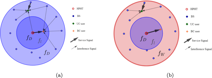

  

  Different proposed scenarios. a Scenario 1: shared spectrum b Scenario 2: dedicated spectra

• (b) Inside users fed by the HPHT suffer from interference from outside BS. However, this interference is variable depending on the distance from HPHT and can be significantly small for non-edge users.

• (c) Outside users fed by the UC BSs suffer from interference from the HPHT even if they are out of the BC coverage. Indeed, these outside users are receiving signals from both outside BSs and HPHT at the same frequency. However, the level of interference perceived by an outside UC user from a HPHT depends on its distance to the HPHT. Particularly, it can be significantly small if (i) the broadcast area is large enough, and the power of HPHT is properly designed or (ii) the UC receiver is really far from the HPHT. It is worth mentioning that the signals received from HPHT and BS are not synchronized; hence, a UC user will consider the HPHT signal as interference.

• (d) The interest of this scheme is clearly seen in terms of bandwidth allocation as inside and outside users (of the broadcast area) with TV services are operating at the same frequency. This will be at the detriment of additional interference level as explained above.

The SINR for inside users is given by

$$ S_{{\mathrm{i}}}=\frac{P_{{\mathrm{D}}} g r_{v}^{-\beta}}{\sigma^{2}+I_{{\mathrm{D}}}} $$

(1)

where P_D is the transmission power by the HPHT, g represents the random channel effect between the HPHT and the user, including shadowing and fading. r_v is the distance between the HPHT and the user, β represents the path loss exponent for broadcast, σ² is the noise power, and I_D denotes the interference on an inside user from outside BS. The interference is the sum of the powers of the received interfering signals. For a user in the broadcast area operating at frequency f_D, all BSs in the UC area are considered as interferers, then I_D is given by

$$ I_{{\mathrm{D}}}=\sum \limits_{j\in \Phi} P_{{\mathrm{L}}} \; h \; r_{s,j}^{-\alpha} $$

(2)

where P_L is the transmission power of UC BS, h represents the channel random effect between the BS and the user, r_s,j is the distance between a user and interfering BS j and Φ is the set of all outside BS. Note that in regular networks, the interference is weighted by the probability of having the interfering BS transmitting at a time. Such probability has its own distribution as the one used in [39]. However, for the case of linear services, it can be assumed that there is always packets being sent based on the nature of the service.

The SINR for outside users is given by:

$$ S_{o}=\frac{P_{{\mathrm{L}}} h r_{l}^{-\alpha}}{\sigma^{2}+I_{1}+I_{2}} $$

(3)

where r_l is the distance between the serving BS and the user, α represents the path loss exponent for UC, σ² is the noise power, and I₁ and I₂ denote the interference on an outside user from outside BS and the HPHT, respectively. Note that it is known that the interference in such models is much bigger than the noise power and it is known to be the limiting factor for the performance. The interference on a user from interfering BS is given by

$$ I_{1}=\sum \limits_{j\in \Phi/b} P_{{\mathrm{L}}} \; h \; r_{q,j}^{-\alpha} $$

(4)

and from the HPHT transmitter is given by

$$ I_{2} = B_{{\mathrm{R}}} P_{{\mathrm{D}}} \; g \; r_{{\mathrm{d}}}^{-\beta} $$

(5)

where Φ/b denotes the set of all BSs in the UC area excluding the serving BS for user under consideration. r_q,j is the distance from an outside user and interfering BS j, and r_d is the distance from an inside user to the HPHT transmitter. B_r is the ratio between the BW of the BC and that of UC. Since, in general, the bandwidth (BW) of the BB network is higher than that of the BC where both are overlapping, the ratio can be written as following:

$$ B_{{\mathrm{R}}}={\text{min}} \left(1,\frac{{\mathrm{BW_{BC}}}}{{\mathrm{BW_{UC}}}}\right) $$

(6)

where BW_BC and BW_UC are the BW of BC and UC, respectively. This term is added to count only the overlapping spectrum when calculating the total interference power. For example, DVB-T2 operates at 8 MHz of bandwidth, and LTE-A usually operates at 10 MHz or 20 MHz of bandwidth.

2.2 Scenario 2: dedicated spectrum scenario

The second scenario considered in this paper differs from scenario 1 in the spectrum allocation. Indeed, here, the BC HPHT operates at f_D, UC BS inside BC area operate at f_L, while the BS outside BC domain operate at f_W, a sub-band of the TV white space, where f_L,f_W, and f_D do not overlap. This scenario is summarized in Fig.2b. This will result in the following points:

• (a) Compared to shared spectrum scenario, ICI for UC is significantly reduced due to the usage of three different frequencies.

• (b) Contrarily to scenario 1, inside users, fed by the HPHT will only be limited by path loss and noise, and will not suffer from any interference.

• (c) Outside users fed by the UC BS suffer only from ICI produced by outside cells.

• (d) The interference is limited at the expense of additional bandwidth allocation.

The SNR for inside users is given by

$$ S_{{\mathrm{i}}}=\frac{P_{{\mathrm{D}}} g r_{v}^{-\beta}}{\sigma^{2}} $$

(7)

The SINR for outside users is given by

$$ S_{{\mathrm{o}}}=\frac{P_{{\mathrm{L}}} h r_{l}^{-\alpha}}{\sigma^{2}+I_{1}} $$

(8)

The difference from shared spectrum scenario is that I_D, the interference from outside BS on inside users, and I₂, the interference from HPHT on outside users, are both eliminated from the equations.

2.3 PDFs of main separation distances

Three distances shown in Fig. 3 are particularly important in the derivations that will follow: (1) the distance r_d between the UC user and the HPHT transmitter, (2) the distance r_v between a BC user and the center, and (3) the distance r_l between a UC user and its serving BS. Since both BS and users positions are random, the distances between the transmitters and the receivers such as r_l,r_d,r_q,r_v, and r_s are random variables, and their distributions are needed in the derivation of coverage and capacity.

Fig. 3

Important distances used in the model

The CDF of r_d is given by

$$ \begin{aligned} F_{r_{{\mathrm{d}}}}(R_{{\mathrm{d}}}) & = \mathbb{P}\left[r_{{\mathrm{d}}}<R_{{\mathrm{d}}}\right]\\ & =\frac{A(R_{{\mathrm{d}}},r_{{\mathrm{b}}})}{A_{{\text{UC}}}}\\ & =\frac{\pi R_{{\mathrm{d}}}^{2} -\pi r_{{\mathrm{b}}}^{2}}{\pi r_{{\text{max}}}^{2} - \pi r_{{\mathrm{b}}}^{2}}\\ & = \frac{1}{r_{{\text{max}}}^{2} -r_{{\mathrm{b}}}^{2}} R_{{\mathrm{d}}}^{2} -\frac{r_{{\mathrm{b}}}^{2}}{r_{{\text{max}}}^{2} -r_{{\mathrm{b}}}^{2}} \end{aligned} $$

(9)

where A(R_d,r_b) is the area limited by the two circles of radius R_d and r_b. The PDF of r_d will then be

$$ \begin{aligned} f_{r_{{\mathrm{d}}}}(r_{{\mathrm{d}}}) & = \frac{d F_{r_{{\mathrm{d}}}}(r_{{\mathrm{d}}})}{d r_{{\mathrm{d}}}}\\ & =\frac{2}{r_{{\text{max}}}^{2} -r_{{\mathrm{b}}}^{2}} r_{{\mathrm{d}}} \end{aligned} $$

(10)

Similarly, the PDF of r_v is given by

$$ f_{r_{{\mathrm{v}}}}(r_{{\mathrm{v}}}) = \frac{2}{r_{{\mathrm{b}}}^{2}} r_{{\mathrm{v}}} $$

(11)

r_l represents the distance to the serving BS. That means that the area between the user and the serving BS is empty from any interfering BS. For a PPP in $\mathbb {R}^{2}$, the null probability in an area A is $\exp (-\lambda A)$ [35]. Then, the Complementary Cumulative Distribution Function (CCDF) of r_l is as following:

$$ {\begin{aligned} F_{r_{{\mathrm{l}}}}(R_{l}) & = \mathbb{P}\left[r_{{\mathrm{l}}}<R_{{\mathrm{l}}}\right]\\ & = 1-\exp(-\lambda A)\\ & = 1-\exp(-\lambda \int \limits_{\max(r_{{\mathrm{b}}},r_{{\mathrm{d}}}-R_{{\mathrm{l}}})}^{\min(r_{{\text{max}}},r_{{\mathrm{d}}}+R_{{\mathrm{l}}})} 2 \theta v \; dv)\\ & = 1-\exp\left(-2 \lambda \int \limits_{\max(r_{{\mathrm{b}}},r_{{\mathrm{d}}}-R_{{\mathrm{l}}})}^{\min(r_{max},r_{d}+R_{{\mathrm{l}}})}\text{arccos}\left(\frac{v^{2}+r_{{\mathrm{d}}}^{2}-R_{{\mathrm{l}}}^{2}}{2 v\; r_{{\mathrm{d}}}}\right) v dv\right)\\ \end{aligned}} $$

(12)

Then, the PDF of r_l is given by

$$ {\begin{aligned} f_{r_{{\mathrm{l}}}}(r_{{\mathrm{l}}}) = \frac{d}{dr_{{\mathrm{l}}}} \left[ {\text{exp}}\left(-2 \lambda \int\limits_{\max(r_{{\mathrm{b}}},r_{{\mathrm{d}}}-r_{{\mathrm{l}}})}^{\min(r_{{\text{max}}},r_{{\mathrm{d}}}+r_{{\mathrm{l}}})} \text{arccos}\left(\frac{v^{2}+r_{{\mathrm{d}}}^{2}-r_{{\mathrm{l}}}^{2}}{2 v\; r_{{\mathrm{d}}}}\right) v dv)\right) \right] \end{aligned}} $$

(13)

where the area A could be found as shown in Fig. 4.

Fig. 4

Calculation of area limited by the circle of radius R_l, service area circle, and broadcast area circle

Approximation of the PDF ofr_l: Eq. (13) is very hard to express and interpret, and therefore will be hard to be used in the sequel. This exact expression is needed in the following cases:

• The density of the BSs is extremely low, so that the cell sizes are comparable to the large BC zone.

• For the users on the BC/BB border.

• For the users on the edge of the service area.

In all of these cases, the BC zone disturbs the user arrangement around the BS. Now since the first case is impractical, and the number of users on the border is relatively small, and since the service area edge is hypothetical for calculation purposes, an approximation with the conventional PDF presented in [31] can be made. Thus the PDF of r_l could then be reduced to

$$ f^{*}_{r_{{\mathrm{l}}}}(r_{{\mathrm{l}}}) = 2 \pi \lambda r_{{\mathrm{l}}}~\text{exp}\left(-\pi \lambda r_{{\mathrm{l}}}^{2}\right) $$

(14)

It can clearly be seen that even though the approximation is much simpler than the exact value, it completely ignores the relative position to the center and the broadcast radius r_b. In the sequel, this approximation will be used when necessary, like in the estimation of coverage probability for BC users in (17) and (32) and UC users in (23) and (34), where both the exact formula and the approximation could be used.

3 Probability of coverage

In this section, we derive the analytical expressions for the probability of coverage of inside users (i.e., broadcast region), outside users (i.e., UC region), and the probability of coverage of any user at any position. The probability of coverage is defined as the probability of a user to have a SINR value higher than a certain threshold T [35]. In order to clarify the derivation steps, Table 1 summarizes the used symbols. Since shared spectrum scenario and dedicated spectrum scenario have slight differences in the derivation of final expressions, the derivation for the first scenario is explained, while in the second scenario, only the final result is stated with indication on the differences.

Table 1 Table of used symbols

3.1 Shared spectrum scenario

3.1.1 Coverage for BC users

For inside users under broadcast, the probability of coverage is given by

$$ \begin{aligned} P_{{\text{c/i}}} &= \mathbb{E}_{r_{{\mathrm{v}}}}\left[\mathbb{P} []S_{{\mathrm{i}}}>T|r_{{\mathrm{v}}}\right] ]\\ & = \mathbb{E}_{r_{{\mathrm{v}}}}\left[\mathbb{P} \left[\frac{P_{{\mathrm{D}}} g r_{{\mathrm{v}}}^{-\beta}}{\sigma^{2}+I_{{\mathrm{D}}}}>T|r_{{\mathrm{v}}}\right] \right]\\ & \stackrel{(a)}{=} \int \limits_{0}^{r_{{\mathrm{b}}}}{\mathbb{P} []g>\frac{T r_{{\mathrm{v}}}^{\beta}}{P_{{\mathrm{D}}}}\left(\sigma^{2}+I_{{\mathrm{D}}}\right)|r_{{\mathrm{v}}}] f_{r_{{\mathrm{v}}}}(r_{{\mathrm{v}}}) d r_{{\mathrm{v}}}}\\ & = \frac{2}{r_{{\mathrm{b}}}^{2}} \int \limits_{0}^{r_{{\mathrm{b}}}}{\mathbb{P} \left[g>\frac{T r_{{\mathrm{v}}}^{\beta}}{P_{{\mathrm{D}}}}\left(\sigma^{2}+I_{{\mathrm{D}}}\right)|r_{{\mathrm{v}}}\right] r_{{\mathrm{v}}} d r_{{\mathrm{v}}}} \end{aligned} $$

(15)

where (a) follows the independence of the distribution of r_v and the channel g. Here, since the interference I_D, which is the sum of the random interference power received from all the BSs, is a random variable, we need to average the probability that g>f(I_D) over that random interference. Now we can derive

$$ {\begin{aligned} \mathbb{P} \left[g>\frac{T r_{{\mathrm{v}}}^{\beta}}{P_{{\mathrm{D}}}}\left(\sigma^{2}+I_{{\mathrm{D}}}\right)|r_{{\mathrm{v}}}\right] & = \mathbb{E}_{I_{{\mathrm{D}}}}\left[ \mathbb{P} [g>\frac{T r_{{\mathrm{v}}}^{\beta}}{P_{{\mathrm{D}}}}\left(\sigma^{2}+I_{{\mathrm{D}}}\right)|I_{{\mathrm{D}}},r_{{\mathrm{v}}}]\right]\\ &\stackrel{(b)}{=} \mathbb{E}_{I_{{\mathrm{D}}}}\left[ {\text{exp}}\left(\frac{- \tau T r_{{\mathrm{v}}}^{\beta}}{P_{{\mathrm{D}}}}\left(\sigma^{2}+I_{{\mathrm{D}}}\right)\right)\right]\\ &= {\text{exp}}\left(\frac{- \tau T r_{{\mathrm{v}}}^{\beta} \sigma^{2} }{P_{{\mathrm{D}}}}\right) \mathbb{E}_{I_{{\mathrm{D}}}}\left[ {\text{exp}}\left(\frac{- \tau T r_{{\mathrm{v}}}^{\beta}}{P_{{\mathrm{D}}}} I_{{\mathrm{D}}}\right)\right]\\ &= {\text{exp}}\left(\frac{- \tau T r_{{\mathrm{v}}}^{\beta} \sigma^{2} }{P_{{\mathrm{D}}}}\right) \mathcal{L}_{I_{{\mathrm{D}}}}\left(\frac{\tau T r_{{\mathrm{v}}}^{\beta}}{P_{{\mathrm{D}}}}\right) \end{aligned}} $$

(16)

where (b) follows the assumption of an exponential distribution of g: $g\thicksim {\text {exp}}(\tau)$. $\mathcal {L}_{I_{{\mathrm {D}}}}(s)$ is the Laplace transform of I_D evaluated at s. Then,

$$ P_{{\mathrm{c/i}}} = \frac{2}{r_{{\mathrm{b}}}^{2}} \int \limits_{0}^{r_{{\mathrm{b}}}}{ {\text{exp}}\left(\frac{- \tau T r_{v}^{\beta} \sigma^{2} }{P_{{\mathrm{D}}}}\right) \mathcal{L}_{I_{{\mathrm{D}}}}\left(\frac{\tau T r_{{\mathrm{v}}}^{\beta}}{P_{{\mathrm{D}}}}\right) r_{{\mathrm{v}}} d r_{{\mathrm{v}}}} $$

(17)

The exact derivation for the Laplace transform $\mathcal {L}_{I_{{\mathrm {D}}}}(s)$ results in the following formula:

$$ {\begin{aligned} \mathcal{L}_{I_{{\mathrm{D}}}}\left(\frac{\tau T r_{{\mathrm{v}}}^{\beta}}{P_{{\mathrm{D}}}}\right) &= \exp\left({\vphantom{- \int \limits_{r_{{\mathrm{b}}}-r_{{\mathrm{v}}}}^{r_{{\mathrm{b}}}+r_{{\mathrm{v}}}} \frac{\arccos\left(\frac{r_{{\mathrm{v}}}^{2}+r_{{\mathrm{s}}}^{2}-r_{{\mathrm{b}}}^{2}}{2r_{{\mathrm{v}}} r_{{\mathrm{s}}}}\right)}{1+\frac{\mu P_{{\mathrm{D}}} r_{{\mathrm{s}}}^{\alpha}}{T \tau P_{{\mathrm{L}}} r_{{\mathrm{v}}}^{\beta}}}}}-2\lambda\left({\vphantom{- \int \limits_{r_{{\mathrm{b}}}-r_{{\mathrm{v}}}}^{r_{{\mathrm{b}}}+r_{{\mathrm{v}}}} \frac{\arccos\left(\frac{r_{{\mathrm{v}}}^{2}+r_{{\mathrm{s}}}^{2}-r_{{\mathrm{b}}}^{2}}{2r_{{\mathrm{v}}} r_{{\mathrm{s}}}}\right)}{1+\frac{\mu P_{{\mathrm{D}}} r_{{\mathrm{s}}}^{\alpha}}{T \tau P_{{\mathrm{L}}} r_{{\mathrm{v}}}^{\beta}}}}} \int\limits_{0}^{r_{{\text{max}}}-r_{{\mathrm{v}}}} \frac{\pi r_{{\mathrm{s}}}}{1+\frac{\mu P_{{\mathrm{D}}} r_{{\mathrm{s}}}^{\alpha}}{T \tau P_{{\mathrm{L}}} r_{{\mathrm{v}}}^{\beta}}} d r_{{\mathrm{s}}} \right.\right.\\ &\quad + \int\limits_{r_{{\text{max}}}-r_{{\mathrm{v}}}}^{r_{{\text{max}}}+r_{{\mathrm{v}}}} \frac{\arccos\left(\frac{r_{{\mathrm{v}}}^{2}+r_{{\mathrm{s}}}^{2}-r_{{\text{max}}}^{2}}{2r_{{\mathrm{v}}} r_{{\mathrm{s}}}}\right)}{1+\frac{\mu P_{{\mathrm{D}}} r_{{\mathrm{s}}}^{\alpha}}{T \tau P_{{\mathrm{L}}} r_{{\mathrm{v}}}^{\beta}}} r_{{\mathrm{s}}} d r_{{\mathrm{s}}} \\ &\quad - \int\limits_{0}^{r_{{\mathrm{b}}}-r_{{\mathrm{v}}}} \frac{\pi r_{{\mathrm{s}}}}{1+\frac{\mu P_{{\mathrm{D}}} r_{{\mathrm{s}}}^{\alpha}}{T \tau P_{{\mathrm{L}}} r_{{\mathrm{v}}}^{\beta}}} d r_{{\mathrm{s}}} \\ &\left.\left.\quad - \int \limits_{r_{{\mathrm{b}}}-r_{{\mathrm{v}}}}^{r_{{\mathrm{b}}}+r_{{\mathrm{v}}}} \frac{\arccos\left(\frac{r_{{\mathrm{v}}}^{2}+r_{{\mathrm{s}}}^{2}-r_{{\mathrm{b}}}^{2}}{2r_{{\mathrm{v}}} r_{{\mathrm{s}}}}\right)}{1+\frac{\mu P_{{\mathrm{D}}} r_{{\mathrm{s}}}^{\alpha}}{T \tau P_{{\mathrm{L}}} r_{{\mathrm{v}}}^{\beta}}} r_{{\mathrm{s}}} d r_{{\mathrm{s}}} \right) \right) \end{aligned}} $$

(18)

It is very clear that Eq. (18) could be reduced to simple closed-form expressions; hence, two different approximations are provided as follows.

Approximation 1 of Eq. (18): Here, it is assumed that due to high BC transmission power, interference is not effective beyond certain point, so the effective interference could be reduced to the disk surrounding a user, with a radius equal to the distance of HPHT from that user. In this case, (18) can be written as

$$ \begin{aligned} \mathcal{L}^{*}_{I}\left(\frac{\tau T r_{{\mathrm{v}}}^{\beta}}{P_{{\mathrm{D}}}}\right) =\exp & \left({\vphantom{\frac{\pi-\text{arccos}\left(\frac{r_{{\mathrm{v}}}^{2}+r_{{\mathrm{s}}}^{2}-r_{{\text{max}}}^{2}}{2r_{{\mathrm{v}}} r_{{\mathrm{s}}}}\right)}{1+\frac{\mu P_{{\mathrm{D}}} r_{{\mathrm{s}}}^{\alpha}}{T \tau P_{{\mathrm{L}}} r_{{\mathrm{v}}}^{\beta}}} r_{{\mathrm{s}}} d r_{{\mathrm{s}}}}}-2\lambda\int\limits_{r_{{\mathrm{b}}}-r_{{\mathrm{v}}}}^{{\text{min}}(r_{{\text{max}}}-r_{{\mathrm{v}}},r_{{\mathrm{v}}})} \right.\\ & \left. \frac{\pi-\text{arccos}\left(\frac{r_{{\mathrm{v}}}^{2}+r_{{\mathrm{s}}}^{2}-r_{{\text{max}}}^{2}}{2r_{{\mathrm{v}}} r_{{\mathrm{s}}}}\right)}{1+\frac{\mu P_{{\mathrm{D}}} r_{{\mathrm{s}}}^{\alpha}}{T \tau P_{{\mathrm{L}}} r_{{\mathrm{v}}}^{\beta}}} r_{{\mathrm{s}}} d r_{{\mathrm{s}}} \right) \end{aligned} $$

(19)

Approximation 2 of Eq. (18): A second approximation could be obtained by assuming that interference is produced by a single interferer placed on the closest point to a user directly on the BC/UC border. This approximation is not generally accurate, but it significantly reduces the complexity of the calculations. The Laplace transform yields:

$$ \mathcal{L}^{**}_{I_{{\mathrm{D}}}}\left(\frac{\tau T r_{{\mathrm{v}}}^{\beta}}{P_{{\mathrm{D}}}}\right) = \frac{1}{1+\frac{\tau P_{{\mathrm{L}}} T r_{{\mathrm{v}}}^{\beta}}{\mu P_{{\mathrm{D}}} (r_{{\mathrm{b}}}-r_{{\mathrm{v}}})^{\alpha}}} $$

(20)

The derivations of the Laplace transform and the approximations could be found in Appendix Appendix 2: Calculation of $\mathcal {L}_{I_{{\mathrm{D}}}}$.

Equation (17) indicates, as expected, that increasing the radius of BC area without a suitable increase in broadcast power will decrease the coverage probability for BC users especially for edge users with a high value of r_v causing both terms inside the integral to be significantly smaller. In fact, the second approximation shown in (19) indicates that the BC radius r_b has a significant additional effect since it appears in the denominator with an exponent which is higher than 2. The equations also indicate that increasing the BS transmission power P_L will reduce the coverage for BC users, with the BS’s density λ has a similar effect.

3.1.2 Coverage for UC users

Outside users are connected to the nearest BS, operating at f_D, and served using unicast. Those users suffer from two sources of interference due to the HPHT power and the other outside BSs. The probability of coverage of the outside users could be written as

$$ {\begin{aligned} P_{{\text{c/o}}} &= \mathbb{E}_{r_{{\mathrm{d}}},r_{{\mathrm{l}}}}\left[ \mathbb{P} [S_{{\mathrm{o}}}>T|r_{{\mathrm{d}}},r_{{\mathrm{l}}} ] \right]\\ & = \mathbb{E}_{r_{{\mathrm{d}}},r_{{\mathrm{l}}}}\left[ \mathbb{P} \left[\frac{P_{{\mathrm{L}}} h r_{{\mathrm{l}}}^{-\alpha}}{\sigma^{2}+I_{1}+I_{2}}> T|r_{{\mathrm{d}}},r_{{\mathrm{l}}} \right] \right]\\ & = \int \limits_{r_{{\mathrm{b}}}}^{r_{{\text{max}}}} f_{r_{{\mathrm{d}}}}(r_{{\mathrm{d}}}) \int \limits_{0}^{2 r_{{\text{max}}}} f_{r_{{\mathrm{l}}}}(r_{{\mathrm{l}}}) \mathbb{P}\left[h>\frac{T r_{{\mathrm{l}}}^{\alpha}}{P}\left(\sigma^{2}+I_{1}+I_{2}\right)|r_{{\mathrm{d}}},r_{{\mathrm{l}}}\right] d r_{{\mathrm{l}}} d r_{{\mathrm{d}}} \end{aligned}} $$

(21)

where the last step follows the independence of the distribution of r_d,r_l. and the channel random effect represented by h. The distance r_d between an outside user and the HPHT varies between r_b in the case of a user on the edge of the broadcast area, and r_max in the case of a user on the edge of the service area. On the other hand, r_l, the distance between an outside user and its serving base station, varies between 0 and 2r_max. However, practically the upper limit is likely much less, especially when the BS density is high enough. Again, the probability of coverage for outside users can be deduced from the previous equation by

$$ {\begin{aligned} & \mathbb{P}\left[h>\frac{T r_{{\mathrm{l}}}^{\alpha}}{P}\left(\sigma^{2}+I_{1}+I_{2}\right)|r_{{\mathrm{d}}},r_{{\mathrm{l}}}\right] \\ & \; = \mathbb{E}_{I_{1}}\left[ \mathbb{E}_{I_{2}}\left[~\text{exp}~\left(\frac{-\mu T r_{{\mathrm{l}}}^{\alpha}}{P_{{\mathrm{L}}}}\left(\sigma^{2} + I1 + I2\right) \right)\right]\right] \\ & \; = \text{exp}\left(\frac{-\mu T r_{{\mathrm{l}}}^{\alpha} \sigma^{2}}{P_{{\mathrm{L}}}}\right) \mathcal{L}_{I_{1}|r_{{\mathrm{d}}}}\left(\frac{\mu T r_{{\mathrm{l}}}^{\alpha}}{P_{{\mathrm{L}}}}\right) \mathcal{L}_{I_{2}|r_{{\mathrm{d}}}}\left(\frac{\mu T r_{{\mathrm{l}}}^{\alpha}}{P_{{\mathrm{L}}}}\right) \end{aligned}} $$

(22)

where the first step follows the independence of the interference from HPHT and the interference from surrounding BSs, and follows also the exponential distribution of the channel parameter h: $h\thicksim {\text {exp}}(\mu)$. Plugging this into (21), and substituting $f_{r_{{\mathrm {d}}}}(r_{{\mathrm {d}}})$ by its formula derived in (10), we get

$$ \begin{aligned} P_{{\mathrm{c/o}}} = {} & \frac{2}{r_{{\text{max}}}^{2}-r_{{\mathrm{b}}}^{2}} \int \limits_{r_{{\mathrm{b}}}}^{r_{{\text{max}}}} r_{{\mathrm{d}}} \int \limits_{0}^{r_{{\text{max}}}} f_{r_{{\mathrm{l}}}}(r_{{\mathrm{l}}}) ~\text{exp}~\left(\frac{-\mu T r_{{\mathrm{l}}}^{\alpha} \sigma^{2}}{P_{{\mathrm{L}}}}\right)\\ & \mathcal{L}_{I_{1}|r_{{\mathrm{d}}},r_{{\mathrm{l}}}}\left(\frac{\mu T r_{{\mathrm{l}}}^{\alpha}}{P_{{\mathrm{L}}}}\right) \mathcal{L}_{I_{2}|r_{{\mathrm{d}}},r_{{\mathrm{l}}}}\left(\frac{\mu T r_{{\mathrm{l}}}^{\alpha}}{P_{{\mathrm{L}}}}\right) d r_{{\mathrm{l}}} d r_{{\mathrm{d}}} \end{aligned} $$

(23)

$\mathcal {L}_{I_{1}|r_{{\mathrm {d}}}}\Big (\frac {\mu T r_{{\mathrm {l}}}^{\alpha }}{P_{{\mathrm {L}}}}\Big)$ and $\mathcal {L}_{I_{2}|r_{{\mathrm {d}}}}\Big (\frac {\mu T r_{{\mathrm {l}}}^{\alpha }}{P_{{\mathrm {L}}}}\Big)$ are the Laplace transform of I₁ and I₂, respectively. $\mathcal {L}_{I_{1}|r_{{\mathrm {d}}}}\big (s\big)$ can be evaluated at certain values of r_l and r_d. The exact derivations, reported in Appendix Appendix 3: Calculation of $\mathcal {L}_{I_{1}}$, lead to the following formula:

$$ {\begin{aligned} \mathcal{L}_{I_{1}|r_{{\mathrm{d}}}}\left(\frac{\mu T r_{{\mathrm{l}}}^{\alpha}}{P_{{\mathrm{L}}}}\right) & = \text{exp}~\left(-2 \lambda \left(\int\limits_{{\text{min}}(r_{{\mathrm{l}}},r_{{\text{max}}}-r_{{\mathrm{d}}})}^{r_{{\text{max}}}-r_{{\mathrm{d}}}} \frac{\pi r_{{\mathrm{q}}}}{1+\frac{1}{T}\Big(\frac{r_{{\mathrm{q}}}}{r_{{\mathrm{l}}}}\Big)^{\alpha}} d r_{{\mathrm{q}}}\right.\right. \\ & \quad + \int\limits_{{\text{max}}(r_{{\mathrm{l}}},r_{{\text{max}}}-r_{{\mathrm{d}}})}^{r_{{\text{max}}}+r_{{\mathrm{d}}}} \frac{\text{arccos}(\frac{r_{d}^{2} +r_{{\mathrm{q}}}^{2} - r_{{\text{max}}}^{2} }{2 r_{{\mathrm{d}}} r_{{\mathrm{q}}}})}{1+\frac{1}{T}\Big(\frac{r_{{\mathrm{q}}}}{r_{{\mathrm{l}}}}\Big)^{\alpha}} r_{{\mathrm{q}}} d r_{{\mathrm{q}}} \\ & \quad\left. \left.- \int\limits_{{\text{max}}(r_{{\mathrm{l}}},r_{{\mathrm{d}}}-r_{{\mathrm{b}}})}^{r_{{\mathrm{d}}}+r_{{\mathrm{b}}}} \frac{\text{arccos}\left(\frac{r_{{\mathrm{d}}}^{2} +r_{{\mathrm{q}}}^{2} - r_{{\mathrm{b}}}^{2} }{2 r_{{\mathrm{d}}} r_{{\mathrm{q}}}}\right)}{1+\frac{1}{T}\left(\frac{r_{{\mathrm{q}}}}{r_{{\mathrm{l}}}}\right)^{\alpha}} r_{{\mathrm{q}}} d r_{{\mathrm{q}}} \right)\right) \end{aligned}} $$

(24)

Approximation of the LT in (24): In order to reduce the complexity of (24), an approximation could be made, by assuming that the major source of interference is due to the first term which represents the disk limited by the BC disk and the service area circle. From the above formula, this will lead the following:

$$ {\begin{aligned} \mathcal{L}^{*}_{I_{1}|r_{{\mathrm{d}}}}\left(\frac{\mu T r_{{\mathrm{l}}}^{\alpha}}{P_{{\mathrm{L}}}}\right) & = {} \text{exp}~\left(-2 \lambda \int\limits_{{\text{min}}(r_{{\mathrm{l}}},r_{{\text{max}}}-r_{{\mathrm{d}}})}^{r_{{\text{max}}}-r_{{\mathrm{d}}}} \frac{\pi r_{q}}{1+\frac{1}{T}\Big(\frac{r_{{\mathrm{q}}}}{r_{{\mathrm{l}}}}\Big)^{\alpha}} d r_{{\mathrm{q}}} \right) \end{aligned}} $$

(25)

On the other hand, $\mathcal {L}_{I_{2}|r_{d}}\big (s\big)$ could be evaluated for certain values of r_d as follows:

$$ \begin{aligned} \mathcal{L}_{I_{2}|r_{{\mathrm{d}}}}\left(s\right) &= \mathbb{E}_{g} \left[ \exp(-s I_{2})\right]\\ &= \mathbb{E}_{g} \left[ \exp(-s B_{{\mathrm{R}}} P_{{\mathrm{D}}} g r_{{\mathrm{d}}}^{-\beta})\right]\\ &= \frac{1}{1+\frac{s B_{{\mathrm{R}}} P_{{\mathrm{D}}} r_{{\mathrm{d}}}^{-\beta}}{\tau}}\\ \end{aligned} $$

(26)

then

$$ \begin{aligned} \mathcal{L}_{I_{2}|r_{{\mathrm{d}}}}\left(\frac{\mu T r_{{\mathrm{l}}}^{\alpha}}{P_{{\mathrm{L}}}}\right) &= \frac{1}{1+\frac{B_{{\mathrm{R}}} T \mu P_{{\mathrm{D}}} r_{{\mathrm{d}}}^{-\beta} r_{{\mathrm{l}}}^{\alpha}}{\tau P_{{\mathrm{L}}}}} \end{aligned} $$

(27)

From the three terms in (24) or from the approximation made in (25), one can conclude that the UC transmission power does not affect the Laplace transform of the inter-cell interference. However, increasing P_L boosts the overall coverage by increasing the other two terms in (23). Moreover, taking into account the approximations done in (14) and (25), the effect of the BS density λ is not similarly clear. From one point, increasing λ_BS increases the linear part in (14), but decreases the exponential parts in (14) and (25). Thus, the overall effect of λ_BS depends on other factors that appear in the exponential and control the decay rate like T and α. Note that for the case of B_r equal to 0, indicating no overlapping, the equation returns to the case where no interference from the BC on the UC exists, and $\mathcal {L}_{I_{2}|r_{{\mathrm {d}}}}\Big (\frac {\mu T r_{{\mathrm {l}}}^{\alpha }}{P_{{\mathrm {L}}}}\Big)$ is meaningless, and the coverage probability will be similar to that scenario 2, which will be later shown in (34).

3.1.3 Coverage for any user in the service area

Since the users are randomly and uniformly distributed over the service area, then the probability of a user to be in the broadcast region is

$$ \begin{aligned} P_{{\mathrm{i}}} & = \frac{A_{{\text{BC}}}}{A_{{\text{total}}}}\\ & = \frac{r_{{\mathrm{b}}}^{2}}{r_{{\text{max}}}^{2}} \end{aligned} $$

(28)

where A_BC is the BC area, and A_total is the service area. Consequently, the probability of a user to be in the UC region domain is

$$ P_{{\mathrm{o}}} = 1- \frac{r_{{\mathrm{b}}}^{2}}{r_{{\text{max}}}^{2}} $$

(29)

and the total probability of coverage for a general user in the service area will be

$$ P_{{\mathrm{c}}} = P_{{\mathrm{i}}} P_{{\mathrm{c/i}}} + P_{{\mathrm{o}}} P_{{\mathrm{c/o}}} $$

(30)

3.2 Dedicated spectrum scenario

The derivation steps of scenario 2 are similar to that of scenario 1 with one major difference: the elimination of I_D and I₂ and their related equations. Thus, the probability of coverage for inside users will be as follows:

$$ P_{{\mathrm{c/i}}} = \frac{2}{r_{{\mathrm{b}}}^{2}} \int \limits_{0}^{r_{{\mathrm{b}}}}{ {\text{exp}}\left(\frac{- \mu T r_{{\mathrm{v}}}^{\beta} \sigma^{2} }{P_{{\mathrm{D}}}}\right) r_{{\mathrm{v}}} d r_{{\mathrm{v}}}} $$

(31)

using equation 3.381/8 in [40], this equation could be written in the form

$$ P_{{\mathrm{c/i}}} = \frac{2}{r_{{\mathrm{b}}}^{2}} \frac{\gamma\left(\frac{2}{\beta},\frac{\mu T \sigma^{2} r_{{\mathrm{b}}}^{\beta}}{P_{{\mathrm{D}}}}\right)}{\beta \left(\frac{\mu T \sigma^{2}}{P_{{\mathrm{D}}}}\right)^{2/\beta}} $$

(32)

where γ(a,x) is the incomplete gamma function given by

$$ \gamma(a,x) = \int \limits_{0}^{x} e^{-v} v^{a-1} dv $$

(33)

In addition, the probability of coverage of outside users could be written as

$$ \begin{aligned} P_{{\mathrm{c/o}}}= {} & \frac{2}{r_{{\text{max}}}^{2}-r_{{\mathrm{b}}}^{2}} \int \limits_{r_{{\mathrm{b}}}}^{r_{{\mathrm{m}ax}}} r_{{\mathrm{d}}} \int \limits_{0}^{r_{{\text{max}}}} f_{r_{l}}(r_{{\mathrm{l}}})~\text{exp}~\left(\frac{-\mu T r_{{\mathrm{l}}}^{\alpha} \sigma^{2}}{P_{{\mathrm{L}}}}\right)\\ & \mathcal{L}_{I_{1}|r_{{\mathrm{d}}}}\left(\frac{\mu T r_{{\mathrm{l}}}^{\alpha}}{P_{{\mathrm{L}}}}\right) d r_{{\mathrm{l}}} d r_{{\mathrm{d}}} \end{aligned} $$

(34)

In scenario 2, one can notice that coverage of inside users is related only to the parameters of the BC, and it is independent of the unicast parameters. In addition, the coverage of outside users is dependent only on UC parameters and r_b. This means that, in general, the coverage of inside and outside users will increase with this model, but at the expense of using an additional frequency band.

4 Average capacity derivation

In this section, we consider the ergodic capacity (achievable rate) for a unit bandwidth. It is also the definition of the average spectral efficiency in bits per second per hertz. As in the previous section, derivations for scenario 1 are described, and the final results of the second scenario follows.

4.1 Shared spectrum scenario

We consider the average capacity for a bandwidth unit to be as follows:

$$ C = \log_{2} [1+{\text{SINR}}] $$

(35)

4.1.1 Capacity for inside users

The average capacity for the inside users served by broadcast can be evaluated as

$$ {\begin{aligned} C_{{\mathrm{i}}} &= {} \mathbb{E}\left[\log_{2}(1+S_{{\mathrm{i}}})\right]\\ &= \mathbb{E}_{\Phi,g}\left[\log_{2}\left(1+\frac{P_{{\mathrm{D}}} g r_{{\mathrm{v}}}^{-\beta}}{\sigma^{2}+I_{{\mathrm{D}}}}\right)\right]\\ & = \int\limits_{0}^{r_{{\mathrm{b}}}} {f_{r_{{\mathrm{v}}}}(r_{{\mathrm{v}}}) \mathbb{E}\left[\log_{2}\left(1+\frac{P_{{\mathrm{D}}} g r_{{\mathrm{v}}}^{-\beta}}{\sigma^{2}+I_{{\mathrm{D}}}}\right)|r_{{\mathrm{v}}}\right] d r_{{\mathrm{v}}}}\\ & \stackrel{(a)}{=} \int\limits_{0}^{r_{{\mathrm{b}}}} {f_{r_{{\mathrm{v}}}}(r_{{\mathrm{v}}}) {\int\limits_{0}^{\infty} {\mathbb{P}\left[\log_{2}\left(1+\frac{P_{{\mathrm{D}}} g r_{{\mathrm{v}}}^{-\beta}}{\sigma^{2}+I_{{\mathrm{D}}}}\right)>t|r_{{\mathrm{v}}}\right]} d t} d r_{{\mathrm{v}}}}\\ &= \int\limits_{0}^{r_{{\mathrm{b}}}} {f_{r_{{\mathrm{v}}}}(r_{{\mathrm{v}}}) {\int\limits_{0}^{\infty} {\mathbb{P}\left[ g> \frac{ \left(2^{t}-1\right)r_{{\mathrm{v}}}^{\beta}}{P_{{\mathrm{D}}}} \left(\sigma^{2}+I_{{\mathrm{D}}}\right)|r_{{\mathrm{v}}}\right]} d t} d r_{{\mathrm{v}}}}\\ &= \int\limits_{0}^{r_{{\mathrm{b}}}} {f_{r_{{\mathrm{v}}}}(r_{{\mathrm{v}}}) {\int\limits_{0}^{\infty} {\mathbb{E}_{I_{{\mathrm{D}}}}\left[~\text{exp}~\left(\frac{ -\tau (2^{t}-1) r_{{\mathrm{v}}}^{\beta}}{P_{{\mathrm{D}}}} \left(\sigma^{2}+I_{{\mathrm{D}}|r_{{\mathrm{v}}}}\right)\right)\right]} d t} d r_{{\mathrm{v}}}}\\ &= \frac{2}{r_{{\mathrm{b}}}^{2}} \int\limits_{0}^{r_{{\mathrm{b}}}} r_{{\mathrm{v}}} \int\limits_{0}^{\infty} ~\text{exp}~\left(\frac{ -\tau \left(2^{t}-1\right)r_{{\mathrm{v}}}^{\beta} \sigma^{2} }{P_{{\mathrm{D}}}}\right) \mathcal{L}_{I_{{\mathrm{D}}}} \left(\frac{ \tau \left(2^{t}-1\right)r_{{\mathrm{v}}}^{\beta}}{P_{{\mathrm{D}}}}\right) d t d r_{{\mathrm{v}}} \end{aligned}} $$

(36)

where (a) follows from

$$ \mathbb{E}\Big[X\Big] = \int\limits_{0}^{\infty} \mathbb{P}\Big(X>x\Big) dx $$

(37)

$\mathcal {L}_{I_{{\mathrm {D}}}} \Big (s\Big)$ is calculated in Appendix Appendix 2: Calculation of $\mathcal {L}_{I_{{\mathrm{D}}}}$. It could be used by substituting s by $\frac { \tau \left (2^{t}-1\right)r_{{\mathrm {v}}}^{\beta }}{P_{{\mathrm {D}}}}$.

4.1.2 Capacity for outside users

Using similar analysis, the average capacity for outside users is given by

$$ {\begin{aligned} C_{{\mathrm{o}}} &= \mathbb{E}_{r_{{\mathrm{d}}},r_{{\mathrm{l}}},h}\Big[ \log_{2}(1+S_{{\mathrm{o}}})\Big]\\ &= \int \limits_{r_{{\mathrm{b}}}}^{r_{{\text{max}}}} f_{r_{{\mathrm{d}}}}(r_{{\mathrm{d}}}) \int\limits_{0}^{2 r_{{\text{max}}}} f_{r_{{\mathrm{l}}}}(r_{{\mathrm{l}}}) \mathbb{E}\left[ \log_{2}\left(1+ \frac{P_{{\mathrm{L}}} h r_{{\mathrm{l}}}^{-\alpha}}{\sigma^{2} + I_{1} +I_{2}} \right)|r_{{\mathrm{d}}},r_{{\mathrm{l}}}\right] d r_{{\mathrm{l}}} d r_{{\mathrm{d}}}\\ &\stackrel{(a)}{=} \int \limits_{r_{{\mathrm{b}}}}^{r_{{\text{max}}}} f_{r_{{\mathrm{d}}}}(r_{{\mathrm{d}}}) \int\limits_{0}^{2 r_{{\text{max}}}} f_{r_{l}}(r_{l}) \int\limits_{0}^{\infty} \mathbb{E}_{I_{1},I_{2}} \Big[ \\ & \quad \quad \quad \quad \quad \text{exp}~\left(\frac{ -\mu (2^{t}-1) r_{{\mathrm{l}}}^{\alpha}}{P_{{\mathrm{L}}}} \left(\sigma^{2} + I_{1} +I_{2}\right) \right) |r_{{\mathrm{d}}},r_{{\mathrm{l}}}\Big] d t d r_{{\mathrm{l}}} d r_{{\mathrm{d}}}\\ &= \frac{2}{r_{{\text{max}}}^{2} -r_{{\mathrm{b}}}^{2}} \int \limits_{r_{{\mathrm{b}}}}^{r_{{\text{max}}}} r_{{\mathrm{d}}} \int\limits_{0}^{2 r_{{\text{max}}}} f_{r_{{\mathrm{l}}}}(r_{{\mathrm{l}}}) \int\limits_{0}^{\infty} \text{exp}~ \left(\frac{ -\mu (2^{t}-1) r_{{\mathrm{l}}}^{\alpha} \sigma^{2} }{P_{{\mathrm{L}}}}\right) \\ & \quad \quad \quad \quad \quad \mathcal{L}_{I_{1}|r_{{\mathrm{d}}}}\left(\frac{\mu (2^{t}-1) r_{{\mathrm{l}}}^{\alpha}}{P_{{\mathrm{L}}}}\right) \mathcal{L}_{I_{2}|r_{{\mathrm{d}}}}\left(\frac{\mu (2^{t}-1) r_{{\mathrm{l}}}^{\alpha}}{P_{{\mathrm{L}}}}\right) d t d r_{l} d r_{{\mathrm{d}}} \end{aligned}} $$

(38)

where (a) follows the exponential distribution of h. The final step follows the independence between I₁ and I₂.

4.1.3 Total average capacity

Similar to the probability of coverage of a user at any position, the average capacity will be

$$ C = P_{{\mathrm{i}}} C_{{\mathrm{i}}} + P_{{\mathrm{o}}} C_{{\mathrm{o}}} $$

(39)

4.2 Dedicated spectrum scenario

In scenario 2, the capacity for inside and outside users are similar to that of model 1, but again, with the elimination of terms related to I_D and I₂. The capacity of inside users could then be derived and written as

$$ C_{{\mathrm{i}}} = \frac{1}{\ln(2)} \frac{2}{r_{{\mathrm{b}}}^{2}} \int\limits_{0}^{r_{{\mathrm{b}}}} r_{v} \int\limits_{0}^{\infty}~\text{exp}~\left(\frac{ -\tau (e^{t}-1)r_{{\mathrm{v}}}^{\beta} \sigma^{2} }{P_{{\mathrm{D}}}}\right) dt dr_{{\mathrm{v}}} $$

(40)

By some rearrangement, and the use of equation 3.327 in [40], the capacity can be written as

$$ C_{{\mathrm{i}}} = \frac{1}{\ln(2)} \frac{2}{r_{{\mathrm{b}}}^{2}} \int\limits_{0}^{r_{{\mathrm{b}}}} r_{{\mathrm{v}}} ~\text{exp}~\left(\frac{\tau \sigma^{2} r_{{\mathrm{v}}}^{\beta}}{P_{{\mathrm{D}}}} \right) \left[-E_{{\mathrm{i}}}\left(-\frac{\tau \sigma^{2} r_{{\mathrm{v}}}^{\beta}}{P_{{\mathrm{D}}}} \right)\right] d r_{{\mathrm{v}}} $$

(41)

where E_i(x) is the exponential integral function given by

$$ E_{{\mathrm{i}}}(x)= - \int \limits_{-x}^{\infty} \frac{e^{-u}}{u} du $$

(42)

Moreover, the capacity for outside users is given by

$$ {\begin{aligned} C_{o} = & \frac{2}{r_{{\text{max}}}^{2}-r_{{\mathrm{b}}}^{2}} \int \limits_{r_{{\mathrm{b}}}}^{r_{{\text{max}}}} r_{{\mathrm{d}}} \int\limits_{0}^{2 r_{{\text{max}}}} f_{r_{{\mathrm{l}}}}(r_{{\mathrm{l}}}) \int\limits_{0}^{\infty} ~\text{exp}~\left(\frac{ -\mu (2^{t}-1) r_{{\mathrm{l}}}^{\alpha} \sigma^{2} }{P_{{\mathrm{L}}}}\right) \\ & \quad \quad \quad \quad \mathcal{L}_{I_{1}|r_{{\mathrm{d}}}}\left(\frac{\mu \left(2^{t}-1\right) r_{{\mathrm{l}}}^{\alpha}}{P_{{\mathrm{L}}}}\right) d t d r_{{\mathrm{l}}} d r_{{\mathrm{d}}} \end{aligned}} $$

(43)

4.3 Effective capacities

All previously calculated capacities are per frequency unit. However, to derive the average user capacity, multiplication by the occupied bandwidth is needed. But for the BC users, the average effective capacity is related to the transmitted bit rate, which is the required capacity for a proper reception of the service or C^req. Hence, the total BC capacity is given by

$$ C^{{\text{BC}}}= \sum \limits_{m \in \mathcal{M}} C^{{\text{req}}} a_{{\mathrm{m}}} $$

(44)

where $\mathcal {M}$ is the set of users within BC region, and a_m a binary variable that is equal to 1 if the SINR for user m named SINR_m is greater or equal to the threshold T and 0 otherwise, thus indicating if user m is receiving the service properly or not.

The average BC capacity in the broadcast area could be then calculated as follows:

$$ \left[C^{{\text{BC}}}\right] = C^{{\text{req}}} P_{{\mathrm{c/i}}} \lambda_{U} \pi r_{{\mathrm{b}}}^{2} $$

(45)

where $\lambda _{U} \pi r_{{\mathrm {b}}}^{2}$ is equal to the average number of users inside BC area.

Similarly, for UC users, the total cell capacity is given by

$$ C_{{\mathrm{n}}}^{{\mathrm{UC,cell}}} = \sum\limits_{m \in \mathcal{C}_{{\mathrm{n}}}} C^{{\text{user}}}_{m} b_{{\mathrm{m,n}}} $$

(46)

where $\mathcal {C}_{{\mathrm {n}}}$ is the set of users in the cell, $C^{{\text {user}}}_{{\mathrm {m}}}$ is the capacity for user m, and b_m is a binary variable that is equal to 1 if user m is connected to the service, i.e., SINR_m>T. $C^{{\text {user}_{m}}}$ could be found as follows:

$$ C^{user}_{m} = N^{RB}_{m} B^{RB} \log_{2}(1+SINR_{m}) $$

(47)

where $N^{RB}_{m}$ is the number of resource blocks allocated to user m, and B^RB is the bandwidth of a single resource block. It is assumed that the resource blocks are uniformly allocated over users like in round robin allocation scheme. So for the UC network, the total capacity will be:

$$ C^{{\text{UC}}}=\sum \limits_{n \in \mathcal{N}} C_{{\mathrm{n}}}^{{\mathrm{UC,cell}}} $$

(48)

Thus, the average UC capacity could be derived as

$$ \left[C^{{\text{UC}}}\right]= \left[N^{{\text{RB}}}\right] B^{{\text{RB}}} C_{{\mathrm{o}}} P_{{\mathrm{c/o}}} \lambda_{U} \pi\left(r_{{\text{max}}}^{2} - r_{{\mathrm{b}}}^{2}\right) $$

(49)

where $\lambda _{U} \pi \left (r_{{\text {max}}}^{2} - r_{{\mathrm {b}}}^{2}\right)$ sums the average number of UC users, and $\left [N^{{\text {RB}}}\right ]$ denotes the average number of resource blocks assigned for a user. Finally, the total average capacity could be given as

$$ \left[C^{{\text{sys}}}\right]=\left[C^{{\text{BC}}}\right]+\left[C^{{\text{UC}}}\right] $$

(50)

Those values are used to derive the capacity of the hybrid system for both scenarios.

4.4 Quality of experience

In this section, we aim at discussing and evaluating the quality of experience (QoE) of the proposed scenarios from one side and linking them with the main design parameters that have been evaluated in the previous sections.

In literature, different standards and studies have been elaborated to quantify the QoE of the TV services as seen by the end-users, and to expand the necessary procedures for such evaluations. Definitely, these approaches differ in aspects and metrics; however, one can distinguish between subjective [41] and objective QoE metrics [42]. While the subjective metrics are very pertinent for the network operators as they are directly obtained by humans. They lack however many important characteristics (such as real time assessment). Moreover, they require huge time and resources. To counteract this problem, researchers have also proposed objective QoE metrics for video services and tried to link them with the QoS delivered by the network. A good example therein would be in relating the video streaming time with the network latency or the QoE with the data rate [43].

In this work, and due to its theoretical aspect, we have adopted two objective QoE scores and linked them with the design metrics detailed in the previous section. Both have been widely accepted by the research community. The two QoE scores are given as follows:

• 1. QoE score 1: In [44], the authors have related the IQX (exponential interdependency of quality of experience and quality of service) hypothesis QoE to the packet loss ratio. In our work, a packet is considered to be lost if the user is not in coverage, i.e., if the SINR of that user is below the threshold T. In other words, the packet loss is directly related to the outage probability (the complementary of coverage). Hence, the first QoE defined in our work, denoted hereafter as Q₁, is related to the probability of coverage as follows:

  $$ Q_{1} = 3.01\;{\text{exp}}(-4.473\;(1-P_{{\mathrm{c}}}))+1.065 $$

  (51)

• 2. QoE score 2: In [45], the authors suggested another QoE score that combines three scores: freezing score, bitrate switch score, and video bit rate score. They are given by

  $$ Q_{2} = Q_{{\mathrm{v}}} + \kappa Q_{{\mathrm{f}}} + \rho Q_{{\mathrm{s}}}; $$

  (52)

  where Q_v is the rate score given by

  $$ Q_{{\mathrm{v}}} = \ln(C) $$

  (53)

  Q_f is the freezing score defined as

  $$ Q_{{\mathrm{f}}} = -\frac{{\text{exp}}(-1+t_{{\mathrm{f}}})}{1+{\text{exp}}(-1+t_{{\mathrm{f}}})} $$

  (54)

  where t_f is the freezing time. A freezing time is the time where the capacity is below the minimum rate required for a video stream. Finally, Q_s is the change in video quality category, and it is defined as

  $$ Q_{{\mathrm{s}}} = \frac{-\nu |{\mathrm{cat_{k}}}-{\mathrm{cat_{k-1}}}|}{{\mathrm{cat_{k}}}} $$

  (55)

  where cat_k and cat_k−1 are the quality categories for current and previous time slots, and, κ,ρ, and ν are all positive weight coefficients. To classify the video quality into categories, we used a table presented by mLAB in [46] that links the video resolution to the minimum required data rate for a proper reception.

5 Simulation results and discussion

To compare the formulations derived previously with simulations, numerical and Monte-Carlo (MC) simulations have been conducted. Numerical analysis was also used to find optimal operating points for different of system parameters. The service area selected is of 30 km radius, with variable BC radius. Unless otherwise mentioned, the density of BSs is equal to 0.15BS/km². Default simulation settings are summarized in Table 2. The isotropic transmission power of BSs is set to 1200 W, and the isotropic transmission power of the HPHT is set to 33 kW. The noise power is set to −105 dBm corresponding to 8 MHz of bandwidth. It is worth mentioning that despite the general framework of our work, the parameters in this paper were selected in line with LTE and DVB specifications [28].

Table 2 Simulation setting

5.1 Simulation and analytical results in terms of coverage CCDF

Firstly, to compare the analytical expressions with MC simulation results, the CCDF of the probability of coverage is calculated for inside users, outside users, and any user in the service area as shown in Fig. 5a–c, respectively, for shared spectrum scenario, and in Fig. 6a–c, respectively, for dedicated spectra scenario.

Fig. 5

General user P_c. CCDF of probability of coverage P_c for shared spectrum scenario a Inside users P_c/ib Outside users P_c/oc General user P_c

Fig. 6

CCDF of probability of coverage P_c for dedicated spectra scenario. a Inside users P_c/ib Outside users P_c/oc General user P_c

Both Figs. 5a and 6a show a very good convergence between the simulation and the analytical results. Figures 5b and 6b show a very high accuracy as well, with error ranging from 1 to 2%. Figures 5c and 6c verify the derived formulations and the different probability expressions in the previous sections. The first approximation for BC users presented in Eq. (19), and the approximation for UC users provided by Eq. (25) produce very close values to both simulation results and derived equations. The second approximation for the BC users provided by Eq. (19) is accurate for high threshold values and looses its accuracy for low threshold values, i.e., below 3 dB. However, the use of these approximations reduces significantly the processing time for the analytical derivations. Fortunately, these approximations work well with the practical transmission parameters.

The problem turns out now to find the optimal set of parameters which maximizes the probability of coverage and users’ capacity.

5.2 Optimization of the hybrid network

Among the different design parameters, it is very clear that the first parameter to optimize is the radius (i.e., the coverage) of the broadcast area for both scenarios. Figure 7a, b shows the probability of coverage vs the BC radius for a general user in the service area for UC BS densities of 0.05 BS/km² and 0.15 BS/km² for both scenarios. The results show that for a small value of r_b, where most users are UC users, the probability of coverage P_c will be limited by the achievable P_c in the UC network. When the BC radius r_b increases, more users are being covered by the BC network and thus the total P_c increases. However, when r_b is increased too much, edge users associated with BC become out of coverage due to high interference, pathloss and noise levels. Optimal values of r_b vary between 8 and 12 km.

Fig. 7

Probability of coverage for both scenarios vs. the BC radius r_b for −105 dBm noise power. a Shared spectrum scenario b Dedicated spectra scenario

Both figures show that the required threshold T has a huge effect on the coverage probability, but a limited effect on the optimal radius of BC area. In addition, results show that for shared spectrum scenario, increasing λ_BS pushes the optimal point towards smaller values. This effect is not as clear in scenario 2. The main reason could be that in scenario 1, adding more UC BS add more interference to BC users, and consequently, limits the BC sub-network efficiency. Moreover, a comparison between the two plots shows that there is no significant difference between the two cases in terms of the optimal radius, and it is limited to a shift of around one kilometer in some cases. Excluding the edge users, BC users in general has a better QoE compared to the UC users.

It is worth mentioning that the extreme values of the broadcast radius r_b in each scenario (i.e., SSS and DSS) depict one of the stand-alone networks behaviors. For instance, in the DSS scenario, setting r_b to 0 km is equivalent to broadband network alone while a very large value of r_b depicts the broadcast network. In both extreme cases of r_b, it is very clear that the stand-alone networks could not provide the best coverage performance. One should also notice that, even though the framework is this paper is applicable to any hybrid solution of networks, the simulation parameters have been selected according to LTE and DVB specifications. In other words, the hybrid proposed solution outperforms each of these networks operating alone.

Similar remarks could be concluded from Fig. 8a, b, showing the total system capacity as a function of r_b for the two values of UC BS density mentioned above. Both figures show that an optimal point can be determined for the set of parameters under test.

Fig. 8

Average system capacity vs. the BC radius r_b for −105 dBm noise power, C^req of 2 Mbps, and 1400 users. a Shared spectrum scenario b Dedicated spectra scenario

Since the average values, in general, could be misleading, and in order to highlight the effect of the position on the coverage, a test was done without the last averaging over position with respect to the center in Eqs. (17) and (23) for scenario 1, and Eqs. (32) and (34) for scenario 2. Figure 9a, b shows a cross-section of the service area, from the center to the edge, with the coverage probability at each point with distance R from the center of the service area, for two different values of λ_BS, and their corresponding optimal BC radius r_b for both scenarios. Results show that BC users have excellent coverage for both cases near the HPHT as expected, but this value drops dramatically for scenario 1 on the BC border due to interference, and the drop is more skewed when the density is higher. In the second scenario, the drop is smoother, and it is not affected by the density of BSs. Moreover, UC has a stable coverage value over most of its region except at both boundaries, with a higher average for higher density network, and with a slight out-performance for the dedicated spectrum scenario. One could mention the main changes in the BC/UC border region. In shared spectrum scenario, users on both sides of the UC/BC borders suffer from severe interference levels, which results in the gap seen in Fig. 9a with a probability of coverage that drops down to 0.11 and 0.1 with λ_BS equal to 0.15 and 0.05 BS/km², respectively. In contrary, this gap is not as significant in Fig. 9b that corresponds to dedicated spectra scenario, as it is limited by the slight change in operating BSs density near the border.

Fig. 9

Probability of coverage as a function of distance from center for two values of λ_BS and their corresponding values of r_b for −105dBm noise power and T = 0 dB. a Shared spectrum scenario b Dedicated spectra scenario

Figure 10a, b shows the achievable capacity by 90% of the users in the service area for both scenarios. Higher UC network density achieves higher capacities, mainly due to the advantage of such networks in providing higher number of access points and then resources. Results also show that for shared spectrum scenario, a dense network requires smaller BC area to achieve its optimal values. On the other side, for the same value of r_b, higher density of BSs provides higher probability of coverage, as detailed in the next subsection. In the dedicated spectra scenario, the density does not affect much the optimal point.

Fig. 10

Achievable user capacity per unit frequency vs. the BC radius r_b for −105 dBm noise power and T = 0 dB. a Shared spectrum scenario b Dedicated spectra scenario

The results so far correspond to a certain fixed value of the HPHT BC transmission power P_D. To study the effect of P_D on the optimal setting, the optimal BC radius is calculated for different values of P_D. The results for shared spectrum scenario are shown in Fig. 11. The results show that as the transmission power increases, the optimal radius increases as well. A larger transmission power for the BC produces more coverage in the BC zone, and consequently, a bigger contribution is needed from the BC network, which increases the optimal radius. This shows how, in practice, the size of the BC zone and the amount of transmitted power can be jointly optimized.

Fig. 11

The Effect of BC transmission power on the optimal BC radius in shared spectrum scenario

5.3 Effect of BS density

The second main design parameter for the hybrid network is the density of the BS providing unicast. To study the effect of the BS’s density on probability of coverage for inside, outside, and general user are calculated for different values of λ_BS for both scenarios under study. For this study r_b is selected to be around the optimal values found in the previous section. The results are shown in Fig. 12.

Fig. 12

Effect of the BSs’ density λ_BS on the probability of coverage. a Shared spectrum scenario b Dedicated spectra scenario

For shared spectrum scenario, in general a low-density network will produce less interference on BC users, and thus those users will have better coverage and capacity. Nevertheless, low-density network means that UC users are on average far from their BS and thus have less coverage and capacity. The growth of coverage for UC users with the increase of λ_BS is faster than the decay of the coverage for BC users, thus the total coverage increases, until a point where further increase does not produce additional capacity or coverage since the interfering BSs are becoming closer to typical UC user. In the setting used here, one can conclude that 0.15 BS/km² is enough for nearly maximum coverage. In dedicated spectrum scenario, however, the density does not affect the inside users’ coverage, and consequently, the total coverage is higher in general. However, scenario 2 does not significantly shift the value on which the coverage becomes stable. In practice, the control of BS density can be done by turning off the service transmission of selected BSs but this leads to a new model of a PPP network which is out-of-scope in this paper. The results for average user capacity and system capacity are highly correlated with that of coverage, so they are not shown. Finally, even if this fact is not detailed in the paper due to limited size, we can state from conducted analysis that the lower the λ_BS, the lesser contribution from the BC network is needed, and therefore the smaller the optimal BC radius.

5.4 Interference cancellation

In all the testings performed so far, the induced interference was fully taken into account as no interference cancellation was supposed to be carried out. In practice, some interference techniques are used to reduce its effect on the performance. Those techniques are out of the scope of this study. However, we are interested in having an insight on how a generic interference cancellation scheme can affect the performance of the hybrid network. To model this generic scheme, we multiplied the total interference by a factor γ, that ranges between 0 (all the interference is cancelled) and 1 (no interference cancellation). In fact, the SINR formulas are slightly modified versions of Eqs. (2) and (3) to include the new factor. For shared spectrum the modified formula for BC and UC users will be respectively as following:

$$ S_{{\mathrm{i}}}=\frac{P_{{\mathrm{D}}} g r_{{\mathrm{v}}}^{-\beta}}{\sigma^{2}+\gamma I_{{\mathrm{D}}}} $$

(56)

and

$$ S_{{\mathrm{o}}}=\frac{P_{{\mathrm{L}}} h r_{{\mathrm{l}}}^{-\alpha}}{\sigma^{2}+\gamma(I_{1}+I_{2})} $$

(57)

Similarly, for dedicated spectra scenario, SINR will be modified but with reduced effect. SINR of BC users will remain unchanged as in Eq. (7), while SINR of UC will be a modification of Eq. (8), and will be as following:

$$ S_{{\mathrm{o}}}=\frac{P_{{\mathrm{L}}} h r_{{\mathrm{l}}}^{-\alpha}}{\sigma^{2}+\gamma I_{1} } $$

(58)

where γ is the reduction factor, and γ≤1. Figure 13 shows the coverage probability for shared spectrum scenario (13a) and dedicated spectra scenario (13b).

Fig. 13

Effect of interference cancellation factor γ on coverage and capacity for both scenarios. a Shared apectrum scenario b Dedicated spectra scenario

Figure 13 shows that for both scenarios, coverage could be enhanced by more than 67% for λ = 0.15 BS/km² and around 37% for λ = 0.05 BS/km² with a cancellation factor of −15 dB. Further cancellation increase, i.e., lower values of γ, will not be as effective as noise becomes the dominant limiting factor. Further studies show that the 15 dB cancellation could achieve around 130% increase in average capacity for a user and around 250% increase in achievable capacity for 90% of users.

Table 3 summarises the effect of the different parameters on the performance of the hybrid network.

Table 3 Summary of the parameter effect

5.5 QoE

In this section, we provide the QoE measures of the two hybrid networks as detailed in Section 4.D. Figure 14 shows the average QoE score 1 of the network as a function of the BC radius r_b. The results show that the DSS scenario outperforms the SSS for both BS density values, and that the optimal value of r_b is slightly smaller for more BS-dense areas. Moreover, it can be easily seen that from QoE point of view, the optimal point of r_b is slightly smaller than those obtained through probability of coverage (see Fig. 7a, b).

Fig. 14

A comparison between the two scenarios based on the QoE score 1

Figure 15 shows the QoE as indicated in Q₂ at each user’s position relative to the coverage area center. In this example, we have considered κ = 8,ρ = 1, and ν = 2. The figure shows the different QoE sub-scores and the final score. It can be seen that the users at the edge of the BC area (marked by a blue line in the figure) suffer the most from the degradation of QoE. Note that the results are provided for the SSS scenario only for simplicity.

Fig. 15

The QoE versus the relative position from the center of the service area for SSS

5.6 Comparison between the two scenarios

The two presented scenarios share most of the design criteria, except the frequency bands occupied by each. While the difference in probability of coverage and system capacity is not significant, edge users in the two scenarios experience very different conditions as can be seen in Fig. 9a, b. As can be concluded from Figs. 5c and 6c for coverage probability and Fig. 8a, b for capacity, dedicated spectra scenario has a slight advantage due to fewer sources of interference. However, this slight advantage comes with a very expensive price in terms of occupied bandwidth, due to the use two frequency bands instead of one. For a fair comparison, let us analyze the two scenarios from the perspective of the global area spectral efficiency defined as

$$ A_{{\mathrm{e}}} = \frac{C^{{\text{sys}}}}{{\mathrm{BW_{total}}} \; \pi r_{{\text{max}^{2}}} } $$

(59)

where BW_total = BW_BC+BW_UC is the total bandwidth. BW_total=18 MHz for the dedicated spectra scenario, and BW_total = 10 MHz in the case of shared spectrum scenario because of the overlapping of the bands. The global area spectral efficiency as a function of the BC radius is shown in Fig. 16.

Fig. 16

Global area spectral efficiency comparison between the two proposed scenarios with and without interference cancellation (SSS = shared spectrum scenario, DSS = dedicated spectra scenario)

The results show that even though dedicated spectrum scenario achieves higher capacity and coverage, but globally, shared spectrum scenario is more efficient. The large distances between the HPHT and UC users from one side, and the BS and BC users from the other side, cause the mutual interference to be limited to the edge users. Hence, cancelling this interference by using dedicated spectra scenario has a limited effect on the coverage and capacity, while the bandwidth used is hugely increased (doubled, or even more depending on the used networks) to attain such goal. This eventually leads to a severe drop of the efficiency in the second scenario. The results also show that dedicated spectral scenario with −10 dB of interference cancellation can reach the efficiency level of shared spectrum scenario with no interference management. Moreover, It can be noticed that the use of more advanced receivers with better interference management has more effect on the shared spectrum scenario doubling the efficiency, whereas the effect on the dedicated spectra scenario is limited because of the fewer number of interference sources in that case.

However, it remains up to the designer to use either choice depending on the available resources and their cost. For example, if the state of the edge users is critical, and the additional BW is available and not costly, then dedicated spectra scenario could again be the preferable network option.

Table 4 briefs the comparison between the shared spectrum scenario (SSS) and the dedicated spectra scenario (DSS).

Table 4 Comparison between the SSS and DSS scenarios

6 Conclusion

The work in this paper introduced two different models for hybrid broadcast/broadband coexistence. The first was based on shared spectrum access while the second was based on dedicated spectrum using TVWS. An analytical formulation for both models in terms of probability of coverage and capacity has been derived, and numerical simulations have verified the accuracy of the derived expressions. To the best of the authors knowledge, this paper presents a first reference work dealing with the optimization of the hybrid network with the coexistence of broadband and broadcast networks, from stochastic geometry perspective, taking into account the inter cell interference.

The results showed that in general, the dedicated spectra scenario produces higher coverage probability for a user in the service area by few percents and higher system capacity as well, with similar percentages. However, since it requires an additional frequency band adopted from the TV white space, a compromise could be made between coverage and spectral resources. Even though the compromise, i.e., the choice of scenario 1 or Scenario 2, could be hard to find, a soft solution where Scenario 1 is applied in general, but TV white space is used for BS on the BC/UC boundaries, can be proposed in the future.

The results also indicated that an optimal broadcast radius could be reached for different operation conditions where coverage or capacity could be maximized. The results showed that this optimal point changes depending on the density of UC BS. It is shown that, for both scenarios, a value of BS density beyond which there is no significant gain in either scenario exists. Moreover, it is shown that some interference cancellation possibly introduced at the end-user level could significantly enhance both coverage and user experience. The two proposed scenarios were also directly compared in terms of are spectral efficiency, where the shared spectrum scenario proved to be much more efficient.

The scenarios discussed here are one of many possible configurations. Future investigations on scenarios like broadcast/multi-cast hybrid network could be explored. Finally, it is expected to consider multi broadcast cells in future research directions.

7 Appendix 1: Useful integrations

In the following derivations an integration on a plane for a function over a disk will be needed.

7.1 Integration over a distinct disk

For a disk C with radius R, and with distance D from the origin, where D>R, the integration of function f over the plane, by moving from Cartesian coordinates to polar coordinates can be expressed as:

$$ \int \limits_{C_{/D}} f(r) = \int \limits_{D-R}^{D+R}{2 \theta r f(r) dr} $$

(60)

By taking an arc strip with length as 2θr as shown in Fig. 17. According to cosine law:

$$ \theta = \text{arccos}~\left(\frac{r^{2}+D^{2}-R^{2}}{2rD} \right) $$

(61)

Fig. 17

Integration over a distinct disk

then the integration will finally be given by:

$$ \int \limits_{C_{/D}} f(r) = \int \limits_{D-R}^{D+R}{2~\text{arccos} \left(\frac{r^{2}+D^{2}-R^{2}}{2rD} \right) r f(r) dr} $$

(62)

7.2 Integration over a inscribing disk

For a disk C with radius R, and with distance D from the origin, where D<R, the integration of function f over the plane can be done by moving from Cartesian to polar coordinates, and is given by

$$ \int \limits_{C_{/D}} f(r) = \int \limits_{0}^{R-D}{2 \pi r f(r) dr} + \int \limits_{R-D}^{R+D}{2 \theta r f(r) dr} $$

(63)

where the first term corresponds to the integration of a circular strip from the origin until the strip hits the disk boundaries, and the second term corresponds to a strip starting from the end of first limit, to the end of the disk. this is shown in Fig. 18. Similar to the section above, the final integration will be

$$ {\begin{aligned} \int\limits_{C_{/D}} f(r) = \int \limits_{0}^{R-D}{2 \pi r f(r) dr} + \int \limits_{R-D}^{R+D}{2~\text{arccos}~\left(\frac{r^{2}+D^{2}-R^{2}}{2rD} \right) r f(r) dr} \end{aligned}} $$

(64)

Fig. 18

Integration over a inscribing disk

8 Appendix 2: Calculation of $\mathcal {L}_{I_{{\mathrm {D}}}}$

The term $\mathcal {L}_{I_{D}|r_{v}}(s)$ could be evaluated as follows:

$$ {\begin{aligned} \mathcal{L}_{I_{{\mathrm{D}}}|r_{{\mathrm{v}}}}(s) &= \mathbb{E}\left[\exp(-sI_{{\mathrm{D}}})\right]\\ &= \mathbb{E}_{\Phi,h}\left[\text{exp}\left(-s \sum\limits_{j\in \Phi} {P_{{\mathrm{L}}} h r_{s,j}^{-\alpha}}\right)\right]\\ &\stackrel{(a)}{=} \mathbb{E}_{\Phi} \left[ \prod \limits_{j} \mathbb{E}_{h}\left[\text{exp}\left(-s P_{{\mathrm{L}}} h r_{s,j}^{-\alpha}\right)\right] \right] \\ &\stackrel{(b)}{=} \mathbb{E}_{\Phi} \left[\prod \limits_{j} \frac{1}{1+\frac{s P_{{\mathrm{L}}}}{\mu r_{{\mathrm{s}}}^{\alpha}}} \right]\\ & \stackrel{(c)}{=} {\text{exp}}\left(-\lambda \int \limits_{\mathcal{O}\backslash \mathcal{G}} 1-\frac{1}{1+\frac{s P_{L}}{\mu r_{{\mathrm{s}}}^{\alpha}}}\right)\\ & \stackrel{(d)}{=} {\text{exp}}\left(-\lambda \int \limits_{\mathcal{O}\backslash \mathcal{G}} \frac{1}{1+\frac{\mu r_{{\mathrm{s}}}^{\alpha}}{s P_{{\mathrm{L}}}}}\right)\\ &= {\text{exp}} \left(\underbrace{ -\lambda \int \limits_{\mathcal{O}}\frac{1}{1+\frac{\mu r_{{\mathrm{s}}}^{\alpha}}{s P_{{\mathrm{L}}}}}}_{{\mathrm{term 1}}} \; + \; \underbrace{ \lambda \int \limits_{\mathcal{G}} \frac{1}{1+\frac{\mu r_{{\mathrm{s}}}^{\alpha}}{s P_{{\mathrm{{\mathrm{L}}}}}}}}_{{\mathrm{term 2}}} \right) \end{aligned}} $$

(65)

where (a) follows the independence of channel effect h from the point process Φ. (b) follows the assumed exponential distribution of h: $h \thicksim {\text {exp}}(\mu)$, and that if x is exponentially distributed random variable with parameter θ then $\mathbb {E}_{x}[\exp (-ax)] = \frac {1}{1+(a/\theta)}$, and (c) follows the probability generating functional (PGFL) of the PPP. The integration at (c) is done over the unicast area, i.e., over the whole service area $\mathcal {O}$, excluding the broadcast area, or the gap $\mathcal {G}$. term1 corresponds to interference hypothetically produced by BSs distributed over the whole service area. However, since BSs inside the BC area operate at different frequency, thus not interfering with the users received signal, a gap in the uniformly distributed interferes appears, and this is managed by term2. The latter corresponds to this gap in interfering BSs’ distribution. Since the integration in both terms are on an inscribing disk the method described in Appendix Appendix 1: Useful integrations, part B, could be used to calculate terms1 and term2 as following:

$$ {\begin{aligned} {\text{term 1}} &= -2\lambda\left(\int\limits_{0}^{r_{{\text{max}}}-r_{{\mathrm{v}}}} \frac{\pi r_{{\mathrm{s}}}}{1+\frac{\mu r_{{\mathrm{s}}}^{\alpha}}{s P_{{\mathrm{L}}}}} d r_{{\mathrm{s}}} + \int\limits_{r_{{\text{max}}}-r_{{\mathrm{v}}}}^{r_{{\text{max}}}+r_{{\mathrm{v}}}} \frac{\arccos\left(\frac{r_{v}^{2}+r_{{\mathrm{s}}}^{2}-r_{{\text{max}}}^{2}}{2r_{{\mathrm{v}}} r_{s}}\right)}{1+\frac{\mu r_{{\mathrm{s}}}^{\alpha}}{s P_{{\mathrm{L}}}}} r_{{\mathrm{s}}} d r_{{\mathrm{s}}} \right) \end{aligned}} $$

(66)

$$ {\begin{aligned} {\text{term 2}} = 2\lambda\left(\int\limits_{0}^{r_{{\mathrm{b}}}-r_{{\mathrm{v}}}} \frac{\pi r_{{\mathrm{s}}}}{1+\frac{\mu r_{{\mathrm{s}}}^{\alpha}}{s P_{{\mathrm{L}}}}} d r_{{\mathrm{s}}} + \int\limits_{r_{{\mathrm{b}}}-r_{{\mathrm{v}}}}^{r_{{\mathrm{b}}}+r_{{\mathrm{v}}}} \frac{\text{arccos}\left(\frac{r_{{\mathrm{v}}}^{2}+r_{{\mathrm{s}}}^{2}-r_{{\mathrm{b}}}^{2}}{2r_{{\mathrm{v}}} r_{{\mathrm{s}}}}\right)}{1+\frac{\mu r_{{\mathrm{s}}}^{\alpha}}{s P_{{\mathrm{L}}}}} r_{{\mathrm{s}}} d r_{{\mathrm{s}}} \right) \end{aligned}} $$

(67)

Plugging term1 and term2 into (65), and substituting s by its value, we then have

$$\begin{aligned} \mathcal{L}_{I_{{\mathrm{D}}}|r_{{\mathrm{v}}}}\left(\frac{\tau T r_{{\mathrm{v}}}^{\beta}}{P_{{\mathrm{D}}}}\right) ={} & \text{exp}\left(-2\lambda\left(\int\limits_{0}^{r_{{\text{max}}}-r_{{\mathrm{v}}}} \frac{\pi r_{{\mathrm{s}}}}{1+\frac{\mu P_{{\mathrm{D}}} r_{{\mathrm{s}}}^{\alpha}}{T \tau P_{{\mathrm{L}}} r_{{\mathrm{v}}}^{\beta}}} d r_{{\mathrm{s}}} \right. \right. \\ & + \int\limits_{r_{{\text{max}}}-r_{{\mathrm{v}}}}^{r_{{\text{max}}}+r_{{\mathrm{v}}}} \frac{\text{arccos}\left(\frac{r_{{\mathrm{v}}}^{2}+r_{{\mathrm{s}}}^{2}-r_{{\text{max}}}^{2}}{2r_{{\mathrm{v}}} r_{{\mathrm{s}}}}\right)}{1+\frac{\mu P_{{\mathrm{D}}} r_{{\mathrm{s}}}^{\alpha}}{T \tau P_{{\mathrm{L}}} r_{{\mathrm{v}}}^{\beta}}} r_{{\mathrm{s}}} d r_{{\mathrm{s}}} \\ & - \int\limits_{0}^{r_{{\mathrm{b}}}-r_{{\mathrm{v}}}} \frac{\pi r_{{\mathrm{s}}}}{1+\frac{\mu P_{{\mathrm{D}}} r_{{\mathrm{s}}}^{\alpha}}{T \tau P_{{\mathrm{L}}} r_{{\mathrm{v}}}^{\beta}}} d r_{{\mathrm{s}}} \\ & \left. \left. - \int \limits_{r_{{\mathrm{b}}}-{\mathrm{r}}_{{\mathrm{v}}}}^{r_{{\mathrm{b}}}+r_{{\mathrm{v}}}} \frac{\arccos\left(\frac{r_{{\mathrm{v}}}^{2}+r_{{\mathrm{s}}}^{2}-r_{{\mathrm{b}}}^{2}}{2r_{{\mathrm{v}}} r_{{\mathrm{s}}}}\right)}{1+\frac{\mu P_{{\mathrm{D}}} r_{{\mathrm{s}}}^{\alpha}}{T \tau P_{{\mathrm{L}}} r_{{\mathrm{v}}}^{\beta}}} r_{{\mathrm{s}}} d r_{{\mathrm{s}}} \right) \right) \end{aligned} $$

First approximation follows the same procedure in Eq. (65) until (d). next step will be by similar yet opposite approach as in Appendix Appendix 1: Useful integrations part (B), integrate over the disk of radius r_v and trimmed by the BC disk, this will produce Eq. (19).

As for second approximation, the steps are as following:

$$ \begin{aligned} \mathcal{L}^{**}_{I_{{\mathrm{D}}}|r_{{\mathrm{v}}}}(s) &= \mathbb{E}[\exp(-sI_{{\mathrm{D}}})]\\ &= \mathbb{E}_{{\mathrm{h}}}\left[\exp(-s {P_{{\mathrm{L}}} h (r_{{\mathrm{b}}}-r_{{\mathrm{v}}})^{-\alpha}})\right]\\ &= \frac{1}{1+\frac{s P_{{\mathrm{L}}}}{\mu (r_{{\mathrm{b}}}-r_{{\mathrm{v}}})^{\alpha}}} \end{aligned} $$

(68)

Finally, substituting s by its value, will produce formula in (20).

9 Appendix 3: Calculation of $\mathcal {L}_{I_{1}}$

$\mathcal {L}_{I_{1}|r_{{\mathrm {d}}}}\big (s\big)$ could be calculated as following:

$$ {\begin{aligned} \mathcal{L}_{I_{1}|r_{{\mathrm{d}}}}\Big(s\Big) & = {} \mathbb{E}_{\Phi,h}\left[ \exp\left(-s \sum \limits_{j\in\Phi/b} P_{{\mathrm{L}}} h r_{q,j}^{-\alpha}\right)\right]\\ & = \mathbb{E}_{\Phi}\left[ \prod \limits_{j\in\Phi/b} \mathbb{E}_{{\mathrm{h}}}\left[ \exp\big(-s P_{{\mathrm{L}}} h r_{q,j}^{-\alpha}\big)\right]\right]\\ & = \mathbb{E}_{\Phi}\left[ \prod \limits_{j\in\Phi/b} \frac{1}{1+\frac{s P_{{\mathrm{L}}} r_{{\mathrm{q}}}^{-\alpha}}{\mu}}\right]\\ & \stackrel{(a)}{=} \text{exp}\left(-\lambda \int\limits_{\mathcal{O}\backslash \mathcal{G}} 1-\frac{1}{1+\frac{s P_{{\mathrm{L}}} r_{{\mathrm{q}}}^{-\alpha}}{\mu}} d r_{q} \right)\\ & = \text{exp}\left(-\lambda \int\limits_{\mathcal{O}\backslash \mathcal{G}} \frac{1}{1+\frac{\mu r_{{\mathrm{q}}}^{\alpha}}{s P_{{\mathrm{L}}}}} d r_{{\mathrm{q}}} \right)\\ & = \text{exp}\left(\underbrace{-\lambda \int\limits_{\mathcal{O}} \frac{1}{1+\frac{\mu r_{{\mathrm{q}}}^{\alpha}}{s P_{{\mathrm{L}}}}} d r_{{\mathrm{q}}}}_{{\mathrm{term 1}}} + \underbrace{\lambda \int\limits_{\mathcal{G}} \frac{1}{1+\frac{\mu r_{{\mathrm{q}}}^{\alpha}}{s P_{{\mathrm{L}}}}} d r_{{\mathrm{q}}}}_{{\mathrm{term 2}}}\right) \end{aligned}} $$

(69)

where (a) also follows the PGFL of the PPP. term1 refers to the interference generated by the whole service area with uniformly distributed BSs, and term2 refers to the gap caused by the absence of interferers in the BC area. term1 integrates over inscribing disk, then the method in Appendix Appendix 1: Useful integrations, part (B) is applied to formulate it as following:

$$ {\begin{aligned} {\mathrm{term 1}} &= -\lambda \left({\vphantom{\int\limits_{{\text{max}}(r_{l},r_{{\text{max}}}-r_{{\mathrm{d}}})}^{r_{{\text{max}}}+r_{{\mathrm{d}}}}}} \int\limits_{{\text{min}}(r_{{\mathrm{l}}},r_{{\text{max}}}-r_{{\mathrm{d}}})}^{r_{{\text{max}}}-r_{{\mathrm{d}}}} \frac{2 \pi r_{{\mathrm{q}}}}{1+\frac{\mu r_{{\mathrm{q}}}^{\alpha}}{s P_{{\mathrm{L}}}}} d r_{{\mathrm{q}}} \right.\\ & \quad \left. + \int\limits_{{\text{max}}(r_{l},r_{{\text{max}}}-r_{{\mathrm{d}}})}^{r_{{\text{max}}}+r_{{\mathrm{d}}}} \frac{2 \text{arccos}\left(\frac{r_{{\mathrm{d}}}^{2} +r_{{\mathrm{q}}}^{2} - r_{{\text{max}}}^{2} }{2 r_{{\mathrm{d}}} r_{{\mathrm{q}}}}\right)}{1+\frac{\mu r_{{\mathrm{q}}}^{\alpha}}{s P_{{\mathrm{L}}}}} r_{{\mathrm{q}}} d r_{{\mathrm{q}}} \right) \end{aligned}} $$

(70)

term 2 integrates over a distinct disk (the gap), and the method in Appendix Appendix 1: Useful integrations, part (A) is used to formulate it as following:

$$ \begin{aligned} {\mathrm{term 2}} = \lambda \int\limits_{{\text{max}}(r_{{\mathrm{l}}},r_{{\mathrm{d}}}-r_{{\mathrm{b}}})}^{r_{{\mathrm{d}}}+r_{{\mathrm{b}}}} \frac{2 \text{arccos}\left(\frac{r_{{\mathrm{d}}}^{2} +r_{{\mathrm{q}}}^{2} - r_{{\mathrm{b}}}^{2} }{2 r_{{\mathrm{d}}} r_{{\mathrm{q}}}}\right)}{1+\frac{\mu r_{{\mathrm{q}}}^{\alpha}}{s P_{{\mathrm{L}}}}} r_{{\mathrm{q}}} d r_{{\mathrm{q}}} \end{aligned} $$

(71)

then, by substituting s by its value we have

$$ {\begin{aligned} \mathcal{L}_{I_{1}|r_{{\mathrm{d}}}}\left(\frac{\mu T r_{{\mathrm{l}}}^{\alpha}}{P_{{\mathrm{L}}}}\right) & = \exp \left(-2 \lambda \left(\int\limits_{{\text{min}}(r_{{\mathrm{l}}},r_{{\text{max}}}-r_{{\mathrm{d}}})}^{r_{{\text{max}}}-r_{{\mathrm{d}}}} \frac{\pi r_{{\mathrm{q}}}}{1+\frac{1}{T}\left(\frac{r_{q}}{r_{{\mathrm{l}}}}\right)^{\alpha}} d r_{q} \right. \right. \\ &\quad + \int\limits_{{\text{max}}(r_{l},r_{{\text{max}}}-r_{{\mathrm{d}}})}^{r_{{\text{max}}}+r_{{\mathrm{d}}}} \frac{\text{arccos}\left(\frac{r_{{\mathrm{d}}}^{2} +r_{{\mathrm{q}}}^{2} - r_{{\text{max}}}^{2} }{2 r_{{\mathrm{d}}} r_{{\mathrm{q}}}}\right)}{1+\frac{1}{T}\left(\frac{r_{{\mathrm{q}}}}{r_{l}}\right)^{\alpha}} r_{{\mathrm{q}}} d r_{{\mathrm{q}}} \\ &\quad \left. \left. - \int\limits_{{\text{max}}(r_{{\mathrm{l}}},r_{{\mathrm{d}}}-r_{{\mathrm{b}}})}^{r_{{\mathrm{d}}}+r_{{\mathrm{b}}}} \frac{\text{arccos}\left(\frac{r_{{\mathrm{d}}}^{2} +r_{{\mathrm{q}}}^{2} - r_{{\mathrm{b}}}^{2} }{2 r_{{\mathrm{d}}} r_{{\mathrm{q}}}}\right)}{1+\frac{1}{T}\left(\frac{r_{{\mathrm{q}}}}{r_{{\mathrm{l}}}}\right)^{\alpha}} r_{{\mathrm{q}}} d r_{{\mathrm{q}}} \right)\right) \end{aligned}} $$

(72)

References

Research Markets, Global Mobile TV Market Size, Market Share, Application Analysis, Regional Outlook, Growth Trends, Key Players, Competitive Strategies and Forecasts, 2017 to 2025 (Research and Markets, Guinness Centre, Ireland, 2017).
C. Wong, G. W. -H. Tan, T. S. T.n Hew, K. -B. Ooi, Can mobile TV be a new revolution in the television industry?. Comput. Hum. Behav.55(Part B), 764–776 (2016).
M. El-Hajjar, L. Hanzo, A survey of digital television broadcast transmission techniques. IEEE Commun. Surv. Tutor.15(4), 1924–1949 (2013).
L. Fay, L. Michael, D. Gómez-Barquero, N. Ammar, M. W. Caldwell, An overview of the atsc 3.0 physical layer specification. IEEE Trans. Broadcast.62(1), 159–171 (2016).
A. Yamada, H. Matsuoka, T. Ohya, R. Kitahara, J. Hagiwara, T. Morizumi, in 2011 IEEE International Symposium on Broadband Multimedia Systems and Broadcasting (BMSB). Overview of isdb-tmm services and technologies (IEEE, 2011), pp. 1–5. https://doi.org/10.1109/bmsb.2011.5954922.
F. Luo, Mobile Multimedia Broadcasting Standards (Springer, Boston, 2009).
3gpp LTE“,”. http://www.3gpp.org/technologies/keywords-acronyms/98-lte. Accessed 2019.
F. Hartung, U. Horn, J. Huschke, M. Kampmann, T. Lohmar, M. Lundevall, Delivery of broadcast services in 3g networks. IEEE Trans. Broadcast.53(1), 188–199 (2007).
F. Hartung, U. Horn, J. Huschke, M. Kampmann, T. Lohmar, MBMS?IP Multicast/Broadcast in 3G Networks. International Journal of Digital Multimedia Broadcasting. 2009:, 1–25 (2009). https://doi.org/10.1155/2009/597848.
D. Lecompte, F. Gabin, Evolved multimedia broadcast/multicast service (embms) in lte-advanced: overview and rel-11 enhancements. IEEE Commun. Mag.50(11), 68–74 (2012).
L. Christodoulou, O. Abdul-Hameed, A. M. Kondoz, Toward an lte hybrid unicast broadcast content delivery framework. IEEE Trans. Broadcast.PP(99), 1–17 (2017).
H Voigt, in Electronics Conference Biennial Baltic. 15TH. Hybrid media and tv delivery using mobile broadband combined with terrestrial/satellite tv (EricssonStockholm, 2016).
P. A. Fam, M. Crussière, J. F. Hélard, P. Bretillon, S. Paquelet, in 2015 International Symposium on Wireless Communication Systems (ISWCS). Global throughput maximization of a hybrid unicast-broadcast network for linear services (IEEE, 2015), pp. 146–150. https://doi.org/10.1109/iswcs.2015.7454316.
J. Calabuig, J. F. Monserrat, D. G?́mez-Barquero, 5th generation mobile networks: A new opportunity for the convergence of mobile broadband and broadcast services. IEEE Commun. Mag.53(2), 198–205 (2015).
C. Singhal, S. De, Energy-Efficient and QoE-Aware TV Broadcast in Next-Generation Heterogeneous Networks. IEEE Commun. Mag.54(12), 142–150 (2016).
P. Unger, T. Kürner, Modeling and performance analyses of hybrid cellular and broadcasting networks. Int. J. Dig. Multimed. Broadcast.2009:, 1–9 (2009). https://doi.org/10.1155/2009/329073.
C. Heuck, An analytical approach for performance evaluation of hybrid (broadcast/mobile) networks. IEEE Trans. Broadcast.56(1), 9–18 (2010).
K. Wang, Z. Chen, H. Liu, Push-based wireless converged networks for massive multimedia content delivery. IEEE Trans. Wirel. Commun.13(5), 2894–2905 (2014).
A. Lykourgiotis, K. Birkos, T. Dagiuklas, E. Ekmekcioglu, S. Dogan, Y. Yildiz, I. Politis, G. O. Tanik, B. Demirtas, A. M. Kondoz, S. Kotsopoulos, Hybrid broadcast and broadband networks convergence for immersive tv applications. IEEE Wirel. Commun.21(3), 62–69 (2014).
N. Cornillet, M. Crussière, J. F. Hélard, in 2012 IEEE 23rd International Symposium on Personal, Indoor and Mobile Radio Communications - (PIMRC). On the hybrid use of unicast/broadcast networks under energy criterion (IEEE, 2012). https://doi.org/10.1109/pimrc.2012.6362539.
L. Polak, D. Plaisner, O. Kaller, J. Milos, T. Kratochvil, in 2016 39th International Conference on Telecommunications and Signal Processing (TSP). Coexistence between dvb-t2-lite and lte downlink networks in advanced mobile fading channels - partial overlapping rf spectrum (IEEE, 2016). https://doi.org/10.1109/tsp.2016.7760920.
I. Cho, I. Lee, Y. Park, Study on coexistence between long term evolution and digital broadcasting services. Int. J. Adv. Sci. Technol.38:, 75–92 (2012).
M. Crussière, C. Douillard, C. Gallard, M. L. Bot, B. Ros, A. Bouttier, A. Untersee, A unified broadcast layer for horizon 2020 delivery of multimedia services. IEEE Trans. Broadcast.60(2), 193–207 (2014).
D. Rother, S. Ilsen, F. Juretzek, in Broadband Multimedia Systems and Broadcasting (BMSB), 2014 IEEE International Symposium On. A software defined radio based implementation of the "tower overlay over lte-a+" system (IEEE, 2014), pp. 1–6. https://doi.org/10.1109/bmsb.2014.6873514.
H. Bawab, P. Mary, J. F. Hélard, Y. Nasser, O. Bazzi, in 2014 IEEE 79th Vehicular Technology Conference (VTC Spring). Global ergodic capacity closed-form expression of coexisting dvb-lte-like systems (IEEE, 2014). https://doi.org/10.1109/vtcspring.2014.7022931.
A. A. Razzac, S. E. Elayoubi, T. Chahed, B. E. Hassan, in 2013 11th International Symposium and Workshops on Modeling and Optimization in Mobile, Ad Hoc and Wireless Networks (WiOpt). Planning of mobile tv service in standalone and cooperative dvb-ngh and lte networks, (2013), pp. 609–614.
A. A. Razzac, S. E. Elayoubi, T. Chahed, B. El-Hassan, in 2013 IEEE 24th International Symposium on Personal, Indoor and Mobile Radio Communications (PIMRC Workshops). Comparison of lte embms and dvb-ngh mobile tv solutions from an energy consumption perspective (IEEE, 2013). https://doi.org/10.1109/pimrcw.2013.6707828.
P. A. Fam, S. Paquelet, M. Crussière, J. F. Hélard, P. Bretillon, in 2016 IEEE International Symposium on Broadband Multimedia Systems and Broadcasting (BMSB). Optimal capacity of hybrid unicast-broadcast networks for mobile tv services (IEEE, 2016). https://doi.org/10.1109/bmsb.2016.7521934.
P. A. Fam, S. Paquelet, M. Crussière, J. F. Hélard, P. Bretillon, Analytical derivation and optimization of a hybrid unicast-broadcast network for linear services. IEEE Trans. Broadcast.62(4), 890–902 (2016).
P. A. Fam, S. Paquelet, M. Crussière, J. F. Hélard, P. Bretillon, On the energy efficiency of hybrid unicast-broadcast networks for mobile tv services. Journee Scientifique URSI-France 2016 Energie et Radiosciences (2016).
M Haenggi, Stochastic Geometry for Wireless Networks (Cambridge University Press, 2012). https://doi.org/10.1017/cbo9781139043816.
M. Haenggi, J. G. Andrews, F. Baccelli, O. Dousse, M. Franceschetti, Stochastic geometry and random graphs for the analysis and design of wireless networks. IEEE J. Sel. Areas Commun.27(7), 1029–1046 (2009).
F. Baccelli, M. Klein, M. Lebourges, S. Zuyev, Stochastic geometry and architecture of communication networks. PTelecommunication Syst.7(1), 209–227 (1997).
W. Lu, M. D. Renzo, in Proceedings of the 18th ACM International Conference on Modeling, Analysis and Simulation of Wireless and Mobile Systems, MSWiM ’15. Stochastic geometry modeling of cellular networks: Analysis, simulation and experimental validation (ACM, 2015), pp. 179–188.
J. G. Andrews, F. Baccelli, R. K. Ganti, A tractable approach to coverage and rate in cellular networks. IEEE Trans. Commun.59(11), 3122–3134 (2011).
X. Ge, B. Yang, J. Ye, G. Mao, C. -X. Wang, T. Han, Spatial spectrum and energy efficiency of random cellular networks. IEEE Trans. Commun.63(3), 1019–1030 (2015).
L. Xiang, X. Ge, C. -X. Wang, F. Y. Li, F. Reichert, Energy efficiency evaluation of cellular networks based on spatial distributions of traffic load and power consumption. IEEE Trans. Wirel. Commun.12(3), 961–973 (2013).
A. Shokair, Y. Nasser, O. Bazzi, J. F. Hélard, M. Crussière, in 2017 9th International Congress on Ultra Modern Telecommunications and Control Systems and Workshops (ICUMT). Near optimal linear-service oriented resource allocation strategy for lte networks (IEEE, 2017). https://doi.org/10.1109/icumt.2017.8255162.
Y. Zhong, X. Ge, H. H. Yang, T. Han, Q. Li, Traffic matching in 5g ultra-dense networks. IEEE Commun. Mag.56(8), 100–105 (2018).
G. Ryzhik, T. Geronimus, Table of Integrals, Series, and Products, Seventh Edition (Academic Press, Cambridge, MA, 2007).
J. S. Lee, On designing paired comparison experiments for subjective multimedia quality assessment. IEEE Trans. Multimed.16(2), 564–571 (2014). URL https://doi.org/10.1109/TMM.2013.2292590.
P. Brooks, B. Hestnes, User measures of quality of experience: why being objective and quantitative is important. IEEE Netw.24(2), 8–13 (2010). https://doi.org/10.1109/mnet.2010.5430138.
T. Wang, A. Pervez, H. Zou, in 2010 3rd IEEE International Conference on Broadband Network and Multimedia Technology (IC-BNMT). Vqm-based qos/qoe mapping for streaming video, (2010), pp. 807–812. URL https://doi.org/10.1109/ICBNMT.2010.5705202.
M. Fiedler, T. Hossfeld, P. Tran-Gia, A generic quantitative relationship between quality of experience and quality of service. IEEE Network. 24(2), 36–41 (2010). https://doi.org/10.1109/mnet.2010.5430142.
W. Huang, Y. Zhou, X. Xie, D. Wu, M. Chen, E. Ngai, Buffer state is enough: Simplifying the design of qoe-aware http adaptive video streaming. IEEE Trans. Broadcast.64(2), 590–601 (2018).
Huawei mLAB, Video as a Basic Service of LTE Networks: Mobile vMOS Requirements. https://www.huawei.com/minisite/4-5g/en/industryjsdc-j.html. Accessed 2019.
Funding
This work has received a French state support granted to the Convergence TV project through the twentieth FUI (transverse inter-ministry funding) program. The authors would also like to thank the “Image & Réseaux” and “Cap Digital” French business clusters for their support of this work.
Author information
Authors and Affiliations
Contributions
AS came up with the initial model and scenarios, completed the analytical derivations, and conducted the simulations. He wrote the majority of this paper. YN, OB, JFH, and MC supported the case study with their deep knowledge about hybrid networks and stochastic geometry. They also gave feedback and helped to improve the writing. All authors read and approved the final manuscript.
Corresponding author
Ethics declarations
Competing interests
The authors declare that they have no competing interests.
Additional information
Publisher’s Note
Springer Nature remains neutral with regard to jurisdictional claims in published maps and institutional affiliations.
Rights and permissions
Open Access This article is licensed under a Creative Commons Attribution 4.0 International License, which permits use, sharing, adaptation, distribution and reproduction in any medium or format, as long as you give appropriate credit to the original author(s) and the source, provide a link to the Creative Commons licence, and indicate if changes were made. The images or other third party material in this article are included in the article’s Creative Commons licence, unless indicated otherwise in a credit line to the material. If material is not included in the article’s Creative Commons licence and your intended use is not permitted by statutory regulation or exceeds the permitted use, you will need to obtain permission directly from the copyright holder. To view a copy of this licence, visit http://creativecommons.org/licenses/by/4.0/.
About this article
Cite this article
Shokair, A., Nasser, Y., Bazzi, O. et al. On the coexistence of broadcast and unicast in hybrid networks for the transmission of video services using stochastic geometry. J Wireless Com Network 2020, 62 (2020). https://doi.org/10.1186/s13638-020-01670-z
Received:
Accepted:
Published:
DOI: https://doi.org/10.1186/s13638-020-01670-z