Distributed algorithm under cooperative or competitive priority users in cognitive networks

Abstract

Opportunistic spectrum access (OSA) problem in cognitive radio (CR) networks allows a secondary (unlicensed) user (SU) to access a vacant channel allocated to a primary (licensed) user (PU). By finding the availability of the best channel, i.e., the channel that has the highest availability probability, a SU can increase its transmission time and rate. To maximize the transmission opportunities of a SU, various learning algorithms are suggested: Thompson sampling (TS), upper confidence bound (UCB), ε-greedy, etc. In our study, we propose a modified UCB version called AUCB (Arctan-UCB) that can achieve a logarithmic regret similar to TS or UCB while further reducing the total regret, defined as the reward loss resulting from the selection of non-optimal channels. To evaluate AUCB’s performance for the multi-user case, we propose a novel uncooperative policy for a priority access where the kth user should access the kth best channel. This manuscript theoretically establishes the upper bound on the sum regret of AUCB under the single or multi-user cases. The users thus may, after finite time slots, converge to their dedicated channels. It also focuses on the Quality of Service AUCB (QoS-AUCB) using the proposed policy for the priority access. Our simulations corroborate AUCB’s performance compared to TS or UCB.

1 Introduction

1.1 Cognitive radio

The static spectrum allocation has nowadays become a major problem in wireless networks as it results in an inefficient use of the spectrum and can generate holes or white spaces therein. The opportunistic spectrum access (OSA) concept aims at reducing the inefficient use of the spectrum by sharing available spectrum of primary users (PUs), i.e., licensed users who have full access to a frequency band, with opportunistic users called secondary users (SUs). According to OSA, a SU may at any time access an unoccupied frequency band, but it must abandon the targeted channel whenever a PU restarts its transmission in its channel. Indeed, OSA optimizes the use of the spectrum with minimum impacts on PUs and minimizing interference among SUs. OSA is an important strategy for the cognitive radio (CR) [1]; indeed, a CR unit must execute a cognitive cycle in order to implement an OSA strategy. The main three steps of the cognitive cycle are as follows:

• Spectrum sensing: A cognitive radio should be able to sense and detect possible holes in the spectrum. Indeed, the main challenge of a CR is to obtain an accurate status of the spectrum bandwidths (vacant/busy), so that a SU can access a vacant channel without interfering with the transmission of PUs. In the literature, several spectrum sensing algorithms have been proposed to detect primary users’ activities, such as cumulative power spectral density (CPSD) [2], energy detection (ED) [3–6], or waveform-based sensing (WBS) [7, 8].

• Learning and information extraction: This function generates a clear vision about a RF (radio frequency) environment. As a result, a spectrum environment database is constructed and maintained. This database is used to optimize and adapt transmission parameters. The learning and information extraction capabilities of a CR can be achieved using learning algorithms, such as Thompson sampling (TS) [9], upper confidence bound (UCB) [10], and ε-greedy [11]. In [12], we proposed a learning algorithm based on the UCB that monitors the quality of service UCB (QoS-UCB) for the multi-user case. In this paper, we have also developed the QoS aspect of the new proposed AUCB (Arctan-UCB) algorithm.

• Decision making: Following the learning process, the decision about the occupancy of a spectrum should be made to access a particular spectrum bandwidth. Any good decision should depend on the environment parameters as well as on the nature of the SUs’ cooperative or competitive behaviors.

This paper investigates two major scenarios: SUs network with cooperative or competitive behaviors, under two different policies: Side channel [13] and a novel policy called PLA (priority learning access) for the multi-user case.

1.2 Related work

The past decade has witnessed an explosive demand of wireless spectrum that led to the major stress and the scarcity in the frequency bands. Moreover, the radio landscape has become progressively heterogeneous and very complex (e.g., several radio standards, diversity of services offered). Nowadays, the rise of new applications and technologies encourages wireless transmission and accelerates the spectrum scarcity problem. The coming wireless technologies (e.g., 5G) will support high-speed data transfer rates including voice, video, and multimedia.

In many countries, the priority bands for 5G include incumbent users, and it is essential that regulators make high effort to evacuate these frequencies for 5G use—especially in the 3.5 GHz range (3.3–3.8 GHz) [14]. These efforts may consist of (1) putting in place incentives to migrate licensees upstream of frequency allocation, (2) moving licensees to other bands or to a single portion of the frequency range, and (3) allowing licensees to exchange their licenses with mobile operators. When it is not possible to free up a band, the reserving frequencies for 5G bands (i.e., 3.5/26/28 GHz) may lead to the success of 5G services while wasting frequencies. Indeed, according to several recent studies, the frequency sharing approaches represent an efficient solution that can be used to support both potential 5G users and the incumbent users. For instance, the Finnish regulator has chosen to adopt this approach instead of reserving frequencies for the 5G users [14]. Sharing approach will contribute to access new frequencies for 5G in areas where they are needed but underutilized by incumbent users. In this work, we are interested in the opportunistic spectrum access (OSA) that represents a sharing approach in which the SUs can access the frequency bands in opportunistic manner without any cooperation with the PUs.

Before making any decision, a SU should make spectrum sensing process in order to reduce the interference with the primary users. In [15], the authors focus on different spectrum sensing techniques and their efficiency trying to obtain accurate information about the status of the selected channel by a SU at a given time. Moreover, the proposed techniques are analytically evaluated under Gaussian and Rayleigh fading channels. In this work, we focus on the decision making process to help the SU reach the best channel with the highest availability probability. This channel, on the one hand, mitigates any harmful interference with the PU as a result that this channel not often used by this latter. On the other hand, accessing the best channel in the long term can increase the SU’s transmission time and throughput capacity.

Many recent works, in the CR, have attempted to maximize the transmission rate of the secondary user (SU) without generating any harmful interference to the primary user (PU) [16, 17]. To reach this goal, the latter works investigate the effects of using different types of modulation such as OFDM (orthogonal frequency-division multiple access) and SC-FDMA (single-carrier frequency-division multiple access). The main drawback of using OFDM modulation is related to its large peak-to-average power ratio (PAPR) that may increase the interference with the PU. While SC-FDMA has seen as a favorable modulation to maximize the SU’s transmission due to its lower PAPR as well its complexity [18]. Moreover, SC-FDMA is used in several mobile generation such as the third-generation partnership project long-term evolution (3GPP-LTE) and the fourth generation (4G). It is also considered as a promising radio access technology and having an optimal energy-efficient power allocation framework for future generation of wireless networks [19, 20].

In this work, we choose to focus on the multi-armed bandit (MAB) approach in order to help a SU make a good decision, reduce the interference among PU and SU, and maximize the opportunities of this latter. In MAB, the agent may play an arm at each time slot and collect a reward. The main goal of the agent is to maximize its long-term reward or to minimize its total regret, defined as the reward loss resulting from the selection of bad arms. In [21–24], the authors considered the MAB approach in an OSA to improve the spectrum learning¹.

In MAB, the arm reward can be modeled with different models, such as the independent identically distributed (i.i.d.) or Markovian models. In this paper, we focus on the i.i.d. that represents the widely used model for a single user [24, 25] or multi-user case [23, 26, 27].

Based on the MAB problem introduced by Lai and Robbins in [10], the authors of [28] proposed several versions of UCB: UCB1, UCB2, and UCB-normal. All these versions achieve a logarithmic regret with respect to the number of played slots in the single-user case. For multiple users, we proposed respectively in [13] and [29] cooperative and competitive policies to collectively learn the vacancy probabilities of channels and decrease the number of collisions among users. The latter policies are simulated under TS, UCB, and ε-greedy algorithms. The previous simulations were conducted without any proof about the analytical convergences of these algorithms or the number of collisions among SUs. In this work, we show that the same policies achieve a better performance with AUCB compared to several existing algorithms. We also investigate the analytical convergence of these two policies under AUCB, and we show that the number of collisions in the competitive access has a logarithmic behavior with respect to time. Therefore, after a finite number of collisions the users converge to their dedicated channels.

The authors of [30] proposed a distributed learning for multiple SUs called time-division fair share (TDFS) and proved that the proposed method achieves a logarithmic regret with respect to the number of slots. Moreover, TDFS considers that the users can access the channels with different offsets in their time-sharing schedule and each of them achieves almost the same throughput. The work of [31] proposed a musical chair that represents a random access policy to manage the secondary network where the users achieve a different throughput. According to [31], each user selects a random channel up to time T₀ in order to estimate the vacancy probabilities of channels and the number of users U in the network. After T₀, each user randomly selects one of the U best channels. Nevertheless, the musical chair suffers several limitations as follows:

• 1. The user should have a prior knowledge about the number of channels in order to estimate the number of users in the network.

• 2. It cannot be used under the dynamic availability probability since the exploration and exploitation phases are independent.

• 3. It does not take the priority access into account.

To find the U best channels, the authors of [32] proposed a multi-user ε-greedy collision avoiding (MEGA) algorithm based on the ε-greedy previously proposed in [28]. However, the MEGA has the same drawbacks of the musical chair. In the literature, various learning algorithms have been proposed to take into account the priority access, such as selective learning of the kth largest expected rewards (SLK) [33] and kth MAB [34]. SLK is based on the UCB algorithm, while the kth MAB is based on both UCB and ε-greedy.

1.3 Contributions and paper organization

The main contributions of this manuscript are as follows:

• An improved version of UCB algorithm called AUCB: In the literature, several UCB versions have been proposed to achieve a better performance compared to the classical one [28, 35–37]. However, we show that AUCB achieves a better performance compared to previous versions of UCB. By considering the widely used i.i.d. model, the regret for a single or multiple SUs can achieve a logarithmic asymptotic behavior with respect to the number of slots, so that the user may quickly find and access the best channel in order to maximize its transmission time.

• Competitive policy for the priority learning access (PLA): To manage a decentralized secondary network, we propose a learning policy, called PLA, that takes the priority access into account. To the best of our knowledge, PLA represents the first competitive learning policy that successfully handles the priority dynamic access where the number of SUs changes over time [38], while only the priority access or the dynamic access are considered in several learning policies, such as musical chair and dynamic musical chair [31], MEGA [32], SLK [33], and kth MAB [34]. In [38], PLA shows its superiority under UCB and TS compared to SLK, MEGA, musical chair, and dynamic musical chair. In this work, we evaluate the performance of AUCB in the multi-user case based on PLA.

• The upper bound of regret: We analytically prove the asymptotical convergence of AUCB for single or multiple SUs based on our PLA and side channel policies.

• Investigation AUCB’s performance of TS is known to exceed the state of the art in MAB algorithms [35, 39, 40]. Several studies found a concrete bound for its optimal regret [41–43]. Based on these facts, we adopt TS as a reference to evaluate AUCB’s performance.

• We also investigate the QoS of AUCB algorithm under our PLA policy.

Concerning this manuscript’s organization, Section 2 introduces the system model for single and multi-user cases. Section 3 presents the AUCB approach for a single user as well as a novel learning policy to manage a secondary network. AUCB’s performance for both single and multi-user cases are investigated in Section 4. This section also compares the performance of the PLA policy for the multi-user case to recent works. Section 5 concludes the paper.

2 Problem formulation

In this section, we investigate the MAB problem for both single and multi-users cases. We also define the regret that can be used to evaluate a given policy’s performance (Table 1). All parameters used in this section can be found in Table 1.

Table 1 List of notations used through the paper

2.1 Single-user case

Let C be the number of i.i.d. channels where each channel must be in one of two binary states S: S equals 0 if the channel is occupied, and 1 otherwise. For each time slot t, SU should sense a channel in order to see whether it is occupied or vacant and receives a reward r_i(t) from the ith channel. Without any loss of generality, we will then assume that a good decision’s reward, e.g., the channel is vacant, equals to its binary state, i.e., r_i(t) = S_i(t). SU can transmit its data on a vacant channel; otherwise, it must wait for the next slot to sense and use another channel. We suppose that all channels are ordered by their mean availability probabilities, i.e., μ_C≤μ_C−1≤⋯≤μ₁. The availability vector Γ=(μ_i) is initially unknown to the secondary user, but our goal is to estimate it over many sensing slots. If a SU has a perfect knowledge about the channels and their μ_i, then it can select the best available channel, i.e., the first one, to increase its transmission rate. As μ_i is unknown for that user, we will define the regret as the sum of the reward loss due to the selection of a sub-optimal channel at each slot. The regret minimization determines the efficiency of the selected strategy to find the best channel. In a single user case, the regret R(n,β) up to the total number of slots n under a policy β can be defined as follows:

$$ R(n,\beta) = n\mu_{1} - \sum\limits\limits_{t=1}^{n} \mu_{i}^{\beta(t)}(t) $$

(1)

where n is the total number of slots; nμ₁ is the selected channel in an ideal scenario, i.e., when the SU has prior knowledge and always selects the best channel; β(t) denotes the channel selected under the policy β at time t; and $\mu _{i}^{\beta (t)}$ is the mean reward obtained for the i^th channel selected at the time slot t and β(t)=i. The main target of a SU is to estimate the channels availability as soon as possible to attain the highest available one. To reach this goal, UCB was firstly proposed in [10] and applied in [25] to optimize the access over channels and identify the best one with the highest availability probability. UCB contains two dimensions: exploitation and exploration. These latter are respectively represented by X_i(T_i(t)) and A_i(t,T_i(t)).

The index assigned to the ith channel can be defined as follows:

$$ B_{i}\left(t,T_{i}(t)\right)=X_{i}\left(T_{i} (t)\right)+A_{i}(t,T_{i}(t)) $$

(2)

where T_i(t) is the number of times the channel i is sensed by a SU up to the time slot t. The user selects the channel β(t) at slot t that maximizes its index in the previous slot,

$$\beta(t)=\arg \max_{i} \ B_{i}\left(t-1,T_{i}(t-1)\right) $$

After a sufficient time, the user establishes a good estimation of the availability probabilities and thus can converge towards the optimal channel.

2.2 Multi-user case

Let us consider U SUs trying to maximize their network’s global reward. At every time slot t, each user can access a channel when available and transmits its own data. However, multiple SUs can work in cooperative or uncooperative modes. In the cooperative one, the users should coordinate their decisions to minimize the global regret of the network. On the other hand, in a non-cooperative mode, each user independently makes its own optimal decision to maximize its local reward. The regret for the multi-user case, under cooperative or competitive modes, can be written as follows:

$$ R(n,U,\beta) = n\sum\limits\limits_{k=1}^{U} \mu_{k}-\sum\limits\limits_{t=1}^{n} E\left(S^{\beta(t)}(t)\right) $$

(3)

where μ_k is the mean availability of the kth best channel; S^β(t)(t) is defined by the global reward obtained by all users at the time slot t; E(.) represents the mathematical expectation, and β(t) represents all the selected channels² by users at t. We can define S^β(t)(t) by:

$$ S^{\beta(t)}(t) = \sum\limits\limits_{j=1}^{U} \sum\limits\limits_{i=1}^{C} S_{i} (t) I_{i,j} (t) $$

(4)

where the state variable³S_i(t) = 0 indicates that the channel i is occupied by the PU at slot t; otherwise, S_i(t)=1; I_i,j(t) = 1 if the jth user is the sole occupant in channel i at the slot t and 0 otherwise. In the multi-user case, the regret can be affected by the collision among SUs and the channel occupancy which allows us to define the regret for U SUs as shown in the following equation:

$$ R(n,U,\beta) = n \sum\limits\limits_{k=1}^{U} \mu_{k} - \sum\limits\limits_{j=1}^{U} \sum\limits\limits_{i=1}^{C} P_{i,j} (n) \mu_{i} $$

(5)

where $P_{i,j} (n) = \sum \limits _{t=1}^{n} E\left [ I_{i,j}(t)\right ]$ stands for the expectation of times when the user j is the only occupant of the channel i up to n, and the mean of reward can be given by:

$$\mu_{i} = \frac{1}{n}\sum\limits\limits_{t=1}^{n} S_{i}(t)$$

3 Methods

In this section, we present a new approach inspired from the classical UCB in a single-user case, and later on, we generalize our study to consider the case of multi-user. The new approach can find the optimal channel faster than the classical UCB while achieving a lower regret. The classical UCB contains the exploration-exploitation trade-off to find a good estimate of the channels status and converges to the best one (see Eq. (2)). In UCB, a non-linear function for the exploration factor, A_i(t,T_i(t)), is used to ensure the convergence:

$$ A_{i}(t,T_{i}(t))=\sqrt{\frac{\alpha\ln(t)}{T_{i}(t)}} \label {exploration factor} $$

(6)

where α is the exploration-exploitation factor. The effect of α on the classical UCB is well studied in the literature [22, 44, 45]. According to [28, 44, 46, 47], the best value of α should be in the range of [1, 2] in order to make a balance between exploration-exploitation epochs. However, if α decreases, the exploration factor of UCB decreases and the exploitation factor dominates, then the algorithm converges quickly to the channel with the highest empirical reward. All previous works study the effect of A_i(t,T_i(t)) on the UCB with different values of α. In this study, we focus on another form of the exploration factor A_i(t,T_i(t)) based on another non-linear function in order to enhance the convergence to the best channel of the classical UCB. Different non-linear functions of Eq. (6) with similar characteristics can be investigated. We should mention that this function was chosen because it has two main properties:

• A positive function with respect to time t.

• An increasing non-linear function to limit the effect of the exploration.

Therefore, the square-root function introduced in Eq. (6) is widely accepted [24, 28, 46, 47] in order to restrict the exploration factor after the learning phase. Classical UCB ensures the balance between the exploration-exploitation phases at each time slot up to n, using two factors, A_i(t,T_i(t)) and X_i(T_i(t)). Indeed, A_i(t,T_i(t)) is used to explore channels’ availability in order to access the best one with the highest expected availability probability X_i(T_i(t)). The classical UCB gives the same impact of the exploration factor A_i(t,T_i(t)) at each time slot up to n. However, our proposal is based on the idea that the exploration factor A_i(t,T_i(t)) should have an important role during the learning phase while it becomes less important after this period. Indeed, after the learning phase, the user will have a good estimation of channels’ availability, then it can regularly access the best channel. Subsequently, the big challenge is to restrict A_i(t,T_i(t)) after the learning phase by using another non-linear function with the following features:

• It should be an increasing function with a high derivative with respect to time at the beginning to boost the exploration factor during the learning phase in order to accelerate the estimation of channels’ availability.

• It should have a strong asymptotic behavior in order to restrict the exploration factor A_i(t,T_i(t)) under a certain limit, when the user collects some information about channels’ availability.

Subsequently, our study finds that the exploration factor can be adjusted by using the arctan function which has the above features; this proposed UCB version is called AUCB. Indeed, the arctan enhances the convergence speed to the best channel compared to the one obtained with the square-root, and the effect of the exploration factor A_i(t,T_i(t)) can be reduced after the learning phase. The algorithm then gives an additional weight to the exploitation factor X_i(T_i(t)) in the maximization of the index B_i(t,T_i(t)) (see Eq. (2)). In the next section, we will prove that AUCB’s regret has a logarithmic asymptotic behavior.

3.1 AUCB for a single user

This section focuses on the AUCB’s regret convergence for a single user. For the sake of simplicity with regard to the mathematical developments, the regret of Eq. (1) can be written as:

$$\begin{array}{*{20}l} R(n,\beta) =& \sum\limits_{i=1}^{C} E[T_{i}(n)] \mu_{1} -\sum\limits_{i=1}^{C} E[T_{i}(n)] \mu_{i} \\ =&\sum\limits_{i=1}^{C} (\mu_{1}-\mu_{i}) E[T_{i}(n)] \end{array} $$

(7)

where T_i(n) represents the number of time slots that the channel i was sensed by the SU up to the total number of slots n. According to Eq. (7), the regret depends on the channels’ occupancy probability (for stationary channels, the availability probabilities are considered as constant) and the expectation of T_i(n) which is a stationary random variable process. Then, the upper bound of E[T_i(n)] indirectly implies the regret’s upper bound. Subsequently, the regret of our AUCB approach under the single-user case has a logarithmic asymptotic behavior as shown in the following equation (see Appendix A):

$$ R(n,{AUCB}) \leq 8 \sum\limits_{i=2}^{C} \left[ \frac{\ln(n)}{\Delta_{(1,i)}} \right] + \left(1+\frac{\pi^{2}}{3}\right) \sum\limits_{i=1}^{C} \Delta_{(1,i)} $$

(8)

where Δ_(1,i)=μ₁−μ_i represents the difference between the best and worst channels.

3.2 Multi-user case under uncooperative or cooperative access

To evaluate the performance of our proposed algorithm in the multi-user case, we will propose an uncooperative policy for the priority learning access (PLA) to manage a secondary network. We will also prove the PLA’s convergence, as well as the side channel policies with AUCB.

3.2.1 Uncooperative learning policy for the priority access

We investigate the case where the SUs should take decisions according to their priority ranks. In this section, we propose a competitive learning policy that can share the available spectrum among SUs. In addition, we prove the theoretical convergence of the PLA policy with our AUCB approach. In the multi-user case, the big challenge becomes how to collectively learn the channels’ availability for each SU; at the same time, the number of collisions should be set below a certain threshold. Our goal is to ensure that the U users are spread separately to the U best channels. In the classical priority access method, the first priority user SU₁ should sense and access the best channel, μ₁, at each time slot, while the target of the second priority user SU₂ is to access the second best channel. To reach this goal, SU₂ should sense to find the two best channels at the same time, i.e., μ₁ and μ₂, in order to compute their availabilities and thus access the second best channel if available. Similarly, the Uth user should estimate the availability of all U first best channels at each time slot to access the Uth best one. However, it is a costly and impractical method to settle down each user to its dedicated channel. For this reason, we propose PLA where, at each time slot, SU can sense one channel in order to find its dedicated one. In our policy, each user has a dedicated rank, k ∈{1,...,U}, and its target remains the access of the kth best channel. In PLA, each user generates a rank around its prior one to have information about the channels availability, (see Algorithm 1). In this case, the kth user can scan the k best channels and its target is the kth best one. However, if the generated rank of the kth user is different than k, then it accesses a channel that has a vacancy probability in the set {μ₁,μ₂,...,μ_k−1} and may collide with top priority users {SU₁,SU₂,...,SU_k−1}. Moreover, after each collision, SU_k should regenerate its rank in the set {1,...,k}. Thus, after a finite number of iterations, each user settles down to its dedicated channel.

Equation (9) shows that the expectation of collisions in the U best channels E[O_U(n)] for PLA based on our AUCB approach has a logarithmic asymptotic behavior. Therefore, after a finite number of collisions each user may converge to its dedicated channel (see Appendix B):

$$ E[O_{U}(n)] \leq \frac{1-p}{p} \left[ \sum\limits_{k=2}^{U} \left(\frac{8 \ln(n)}{\Delta^{2}_{(k-1,k)}} + 1 + \frac{\pi^{2}}{3} \right)+ \sum\limits_{k=1}^{U} \left(\frac{8 \ln(n)}{\Delta^{2}_{(k,k+1)}} + 1 + \frac{\pi^{2}}{3}\right) \right] $$

(9)

where p indicates the probability of non-collision and Δ_(a,b)=μ_a−μ_b.

We have also proven that the total regret of our policy PLA has a logarithmic asymptotic behavior. It is also worth mentioning that the upper regret bound not only depends on the collisions among users but also on the selection of the worst channels (see Appendix C):

$$ \begin{aligned} R_{PLA}(n,U,{AUCB}) \leq \mu_{1} \left[ \sum\limits_{k=1}^{U} \sum\limits_{i=U+1}^{C} \left(\frac{8\ln(n)}{\Delta_{(k,i)}^{2}} + 1+\frac{\pi^{2}}{3}\right) + E[O_{U}(n)] \right] \end{aligned} $$

(10)

The first term of the above equation reflects the selection of the worst channels while the second one represents the reward loss due to collisions among users in the best channels. The upper bound of the regret presented in Eq. (10) can be affected by three parameters:

• The number of users, U, represented through the first summation, where k denotes the kth best channels for the kth SU.

• The number of channels, C, in the second summation of the regret.

• The total number of time slots, n.

3.2.2 Cooperative learning with side channel policy

The coordination among SUs can enhance the efficiency of their network, instead of dealing with their partial information about the environment. To manage a cooperative network, we propose a policy based on the use of a side channel in order to exchange simple information among SUs with a very low information rate. The side channels are widely used in wireless telecommunication networks to share data among the base-stations [48], and specifically in the context of cognitive network. However, in [49] and [50], the authors considered the cooperative spectrum sharing among PUs and SUs to enhance the transmission rate of the PUs using a side channel.

The signaling channel in our policy is not wide enough to allow high-data rate transmission unlike that used in [49] and [50] which should have a high rate to ensure the data transmission among PUs and SUs. In our policy, the transmission is done over periods. During the first period, i.e., Sub-Slot1, SU₁ (the highest priority user) searches for the best channel by maximizing its index according to Eq. (2). At the same time, and via the secure channel, SU₁ must inform the other users to evacuate its selected channel in order to avoid any collision with them. While avoiding the first selected channel, the second user SU₂ should repeat the same process and so on. If SU₂ does not receive the choice of SU₁ in the first Sub-Slot1 (suppose that SU₁ does not need to transmit during this Sub-Slot), it can directly choose the first suggested channel by maximizing its index B_i,2(t,T_i,2(t)).

To the best of our knowledge, all proposed policies, such as SLK, kth MAB consider a fixed priority, i.e., the kth best channel is reserved for the kth user all the time. Later on, if SU₁ does not transmit for a certain time, then other users cannot select better channels. Subsequently, the main advantages of the cooperation in this policy are as follows:

• An efficient use of the spectrum where best channels are constantly accessed by users.

• An increase in the transmission time of users by avoiding the collision among them.

• Reaching a lower regret compared to several existing policies.

Hence, AUCB’s regret under the side channel policy can achieve a logarithmic efficiency according to the following equation (see Appendix D):

$$ \begin{aligned} R_{SC}(n,U,{AUCB}) \leq \sum\limits_{k=1}^{U} \sum\limits_{i=U+1}^{C} \left[ \underbrace{\frac{8 \ln(n)}{\Delta_{(k,i)}}}_{{Term 1}} + \underbrace{\Delta_{(k,i)} \left(1+\frac{\pi^{2}}{3}\right)}_{{Term 2}}\right] \end{aligned} $$

(11)

where Δ_(k,i)=μ_k−μ_i. k and i, respectively, represent the best and worst channels. The upper bound of this regret contains two terms:

• Term 1 achieves a logarithmic behavior over time.

• Term 2 depends on the vacant channels.

3.3 Quality of service of AUCB

In [12], we study UCB’s quality of service (QoS) for the restless model. The QoS has been studied for both single and multi-users cases using the random rank policy proposed in [23] to manage a secondary network. Based on the QoS-UCB, the user is able to learn channels’ availability and quality.

In this work, we also study the QoS of AUCB using our proposed PLA policy for the priority access of the i.i.d. channels. Supposing that each channel has a binary quality represented by q_i(t) at the slot t: q_i(t)=1 if the channel has a good quality and 0 otherwise. Then, the expected quality collected from the channel i up to n is given as follows:

$$ G_{i}(T_{i}(n)) = \frac{1}{T_{i}(n)}\sum\limits_{\tau=1}^{T_{i}(n)} q_{i}(\tau) $$

(12)

The global mean reward, that takes into account all channels’ quality and availability, can be defined as follows [12]:

$$ \mu_{i}^{Q} = G_{i}(T_{i}(n)).\mu_{i} $$

(13)

The index assigned to the ith channel that takes into account the availability and quality of the ith channel can be defined by:

$$ B_{i}^{Q}(t,T_{i}(t))= X_{i}(T_{i}(t))-Q_{i}(t,T_{i}(t))+A_{i}(t,T_{i}(t))) $$

(14)

According to [12], the term Q_i(t,T_i(t)) that represents the quality factor is given by the following equation:

$$Q_{i}(t,T_{i}(t))=\frac{\gamma M_{i}(t,T_{i}(t)) \ln(t)}{T_{i}(t)} $$

where the parameter γ stands for the weight of the quality factor; M_i(t,T_i(t))=G_max(t)−G_i(T_i(t)) being the difference between the maximum expected quality over channels at time t, i.e., G_max(t), and the one collected from channel i up to time slot t, i.e., G_i(T_i(t)). However, when the ith channel has a good quality G_i(T_i(t)) as well as a good availability X_i(T_i(t)) at time t. Then, the quality factor Q_i(t,T_i(t)) decreases while X_i(T_i(t)) increases. Subsequently, by selecting the maximum of its index $B_{i}^{Q}(t,T_{i}(t))$, the user has a large choice to access the ith channel with a high quality and availability.

To conclude this part, a comparative study in terms of the complexity and convergence speed to the optimal channel has been presented in Table 2 for UCB, AUCB, QoS-UCB, and QoS-AUCB. The latter algorithms behave in $\mathcal {O}(nC)$ for large n and C that represent the number of time slots and channels, respectively. Despite the low complexity of UCB compared to AUCB, this latter can quickly converge to the optimal channel with the highest availability probability.

Table 2 Algorithms complexity

4 Results and discussion

4.1 AUCB’s performance

In our simulations, we will consider that the SU can access a single-available channel at each time slot to transmit its data. In this section, we investigate AUCB’s performance for both single and multi-users cases. Many simulations have been conducted using Monte Carlo methods.

4.1.1 Single user tests

At first, let us consider the simple case of a single SU and let channels’ availability be represented by Γ=[ 0.9 0.8 0.7 0.6 0.5 0.45 0.4 0.3 0.25 0.1]. The percentage of times, P_best, that the SU selects the optimal channel is given by:

$$P_{\text{best}} = 100 \times \sum\limits_{t=1}^{n} \frac{\mathbbm{1}_{{(\beta(t)= \mu_{1}})}}{t} $$

where

$$\mathbbm{1}_{(a=b)}= \left\{\begin{array}{ll} \ 1 \; {if} \; {a =b} \\ \ 0 \; {\text{otherwise}} \end{array}\right. $$

In Fig. 1, P_best shows three parts:

• The first part from 1 to C represents the initialization where the SU plays each channel once to obtain a prior knowledge about the availability of each channel.

  Fig. 1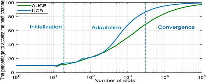

  

  P_best of the two approaches

• The second part from C+1 to 2000 slots represents the adaptation phase.

• In the last part, the user asymptotically converges towards the optimal channel μ₁.

After the initialization part, the two curves evolve in a similar way. After hundreds of slots, the proposed AUCB outperforms the classical UCB. AUCB achieved 65% of the best channel in about 1000 slots, while classical UCB achieved only 45%.

Figure 2 shows AUCB and UCB’s regret factor, evaluated according to Eq. (1) for a single user. As shown in this figure, the regret has a logarithmic asymptotic behavior for the two approaches over time. This result can confirm the theoretical upper bound of regret calculated in Eq. (8) and also presented in Fig. 2, where the upper bound of regret is logarithmic. The same figure shows that AUCB produces a lower regret compared to the classical UCB. This means that our algorithm can rapidly recognize the best channel while the classical UCB required more time to find it.

Fig. 2

Regret of the two approaches

Figure 3 shows the number of times that the two algorithms sense the sub-optimal channels up to time n. For worst channels, our approach and classical UCB have approximately the same behavior. On the other hand, for almost optimal channels (in our example, channels 2 and 3 which respectively have the availability probabilities of 0.8 and 0.7), the UCB could not clearly switch to the optimal channel and spends a lot of time exploring the almost optimal ones.

Fig. 3

Access sub-optimal channels of the two approaches

Figure 4 evaluates AUCB and UCB’s performance with respect to various values of the exploration-exploitation factor α in the interval ]1, 2]. This figure shows that our approach outperforms the classical UCB and achieves a lower regret. Moreover, by increasing α, the classical UCB spends more time to explore the channels in order to find the best channel while our approach can reach the best one with a lower number of slots. The latter result, increases the transmission opportunities for the SU, subsequently decreasing the total regret. In the following sections, we will consider α=1.5.

Fig. 4

Regret of the two approaches with different values of α

4.1.2 Multiple SUs tests

In this section, we consider U=3 with C=10 channels and their availabilities are given by:

Γ=[0.9 0.8 0.7 0.6 0.5 0.45 0.4 0.3 0.2 0.1]. Figure 5 shows the comparison between the regret under the multi-user case defined in Eq. (5) for the two approaches (i.e., UCB and AUCB) under the random rank policy [23]. The latter was used under the UCB; however, it is easy to implement this policy under AUCB to study both algorithms’ performance in the multi-user case.

Fig. 5

Regret comparison for two approaches under the random rank policy

In the random rank policy, when a collision occurs among the users, each of them should generate a random rank in {1,...,U}. Although, both approaches’ regret achieves a logarithmic asymptotic behavior, our algorithm achieves a lower asymptotical regret and converges faster than the classical UCB.

Under the random rank policy, Fig. 6 shows the number of collisions in the U best channels (1, 2, and 3 having availability probabilities of 0.9, 0.8, and 0.7, respectively) for AUCB and classical UCB. Let us remind that, when a collision occurs among users, no-transmission can be achieved and each of them should generate a random rank ∈{1,...,U}. The same figure shows that the number of collisions under a random rank policy with AUCB or classical UCB is quite similar. This can be justified based on a nice random rank policy property; indeed, this policy does not favor any user over another. Therefore, each user has an equal chance of settling down in any of U-best channels. In other word, the random rank policy can naturally achieve a probabilistic fairness access among users. Moreover, in the case of AUCB, the user switches to the optimal channel faster than in the classical one, as shown in Fig. 3 for the single-user case. This fact decreases the number of collisions among users.

Fig. 6

Number of collisions in the best channels under the random rank policy

Figure 7 depicts the regret of AUCB and classical UCB under the side channel policy. As expected, both approaches’ regret increase rapidly at the beginning. At a later time, the increase is slower for the AUCB compared to the classical one. We thus notice that our algorithm presents the smaller regret.

Fig. 7

Regret comparison for two approaches under the side channel policy

4.2 The performance of the PLA policy

This section investigates the performance of the PLA policy under AUCB and UCB compared to the musical chair [31] and SLK [33], and 4 priority users are considered to access the channels based on their prior rank. We then compare UCB and AUCB’s QoS based on the PLA policy.

Figure 8 compares the regret of PLA to SLK and the musical chair policies on a set of 9 channels where PLA achieves the lower regret under AUCB. It is worth mentioning that our policy and SLK take into account the priority access while in the case of the musical chair, users access the channels randomly. As shown in Fig. 8, the musical chair produces a constant regret after a finite number of slots while other methods’ regret is logarithmic. However, during the learning time T₀ in the case of the musical chair, the users randomly access the channels to estimate their availability probabilities as well as the number of users, after that the users just access the U best channels in the long run. Consequently, the musical chair does not follow the dynamism of channels (e.g., assuming that the vacancy probabilities can change with time). The same figure shows that SLK achieves the worst regret.

Fig. 8

PLA, SLK, and musical chair regret

In Table 3, we compare the regret of the four methods with a fixed number of SUs (U=4) and different number of channels (C=5, 9, 13, 17, and 21). As the users spend more time to learn the availability of channels, the regret may increase significantly. This result is due to the access to worst channels and to the collision produced among users. As shown in Table 3, the regret increases with the number of channels, while our PLA policy under AUCB achieves the lowest regret for different considered scenarios (i.e., C = 5, 9, 13, 17, and 21). Thanks to the fact that, under our policy, the SUs quickly learn channels’ vacancy probabilities compared to the others.

Table 3 Regret comparison in the multi-user case with n=10⁵ using the four algorithms PLA-AUCB, PLA-UCB, musical chair, and SLK with a changing number of channels

To study AUCB’s QoS, let us define the empirical mean of the quality collected from channels as follows: G=[0.75 0.99 0.2 0.8 0.9 0.7 0.75 0.85 0.8], then the global mean reward that takes into account the quality as well as the availability Γ_Q can be given by: Γ_Q=[0.67 0.79 0.14 0.48 0.37 0.28 0.22 0.17 0.08]. After estimating channels’ availability and quality (i.e., Γ_Q) and based on the PLA policy, the first priority user SU₁ should converge to the channel that has the highest global mean, i.e., channel 2, while the target of SU₂, SU₃, and SU₄ should respectively be channels 1, 4, and 5. This result can be confirmed in Fig. 9, where the priority users access their dedicated channels in the case of QoS-UCB or QoS-AUCB. Moreover, QoS-AUCB significantly grants users access of their dedicated channels more often than in QoS-UCB.

Fig. 9

Access channels by the priority users using QoS-AUCB and QoS-UCB

Figure 10 diplays the achievable regret of QoS-AUCB and QoS-UCB in the multi-user case. In [12], the performance of QoS-UCB in the restless MAB problem is compared to several learning algorithms, such as the regenerative cycle algorithm (RCA) [51], the restless UCB (RUCB) [52], and Q-learning [53] where Qos-UCB achieved the lowest regret. From Fig. 10, one can notice that the QoS-AUCB policy achieves better performance compared to QoS-UCB.

Fig. 10

QoS-AUCB and QoS-UCB regret

4.3 AUCB compared to Thompson sampling

Thompson sampling has shown its superiority to a variety of versions of UCB and other bandit algorithms [35]. Instead of comparing different versions of UCB to AUCB, in this section, we will study TS and AUCB’ performance in the multi-user case based on the PLA policy for the priority access. We will thus use two factors to make this comparison: access the best channels by each user and the regret that depends not only on the selection of worst-channels but also on the number of collisions among users.

In Fig. 11, we display P_best (the percentage of times where the priority users access successfully their dedicated channels) and the cumulative regret using the PLA policy for 4 SUs based on AUCB, UCB, and TS.

Fig. 11

The performance of AUCB, UCB, and TS

In Figs. 11a, b, the first priority user SU₁ converges to its channel, i.e., the best one, followed by SU₂, SU₃, and SU₄, respectively. Figure 11c compares P_best of the first priority user under AUCB and TS. According to this figure, the first priority user can quickly converge to its dedicated channel using the AUCB algorithm while in the case of TS, the user needs more time to find the best channel. Figure 11d compares the regret of AUCB, UCB, and TS in the multi-user case using the PLA policy for the priority access. However, in TS algorithm, users have to spend more time exploring the C−U worst channels; while in AUCB’s case, the users reach quickly their desired channels. However, a lower regret can increase the successful opportunities of transmission for users. Moreover, selecting dedicated channels in a short period becomes a significant event in a dynamic environment.

5 Conclusion

In this paper, we investigated the problem of opportunistic spectrum access (OSA) in cognitive radio networks, where a SU tries to access PUs’ channels and find the best available channel as fast as possible. We also proposed a new AUCB algorithm to achieve a logarithmic regret with a single user. On the other hand, to evaluate AUCB’s performance in the multi-user case, we proposed a learning policy called PLA for secondary networks that takes into account the priority access. We have also investigated PLA’s performance compared to recent works, such as SLK and the musical chair. We have theoretically found the upper bounds for AUCB’s total regret for a single user as well as for the multi-user case under the proposed policy. Our simulation results show logarithmic regret under AUCB and corroborate AUCB’s performance compared to UCB or TS. It has also been shown that AUCB rapidly converges to the best channel while achieving a lower regret, improving the transmission time and rate of SUs. Moreover, PLA under AUCB can decrease the number of collisions among users under the competitive scenario, thanks to a faster estimation of the channels’ vacancy probability.Like most important works in OSA, this work focused on the independent identical distributed (IID) model in which the state of each channel is supposed to be drawn from an IID process. In future work, we are planning to consider the Markov process that may represent a dynamic memory model to describe the state of available channels; however, it is a more complex process compared to IID. Moreover, our actual model ignores dynamic traffics at the secondary nodes; therefore, the extension of our algorithm to include a queueing-theoretic formulation is desirable. For a more realistic model, the future work will also investigate the effects of using the state of the art of spectrum sensing techniques to detect the activity of the primary users on the performance of the learning and decision-making. Moreover, considering the imperfect sensing, i.e., the probability of false alarm and miss detection, represents a new challenge to developing a more realistic network.

6 Appendix A: Convergence proof of AUCB

In this Appendix, we show that the upper bound of the regret of AUCB is logarithmic with respect to time that means that after a finite time, the user will luckily find and access the best channel with the availability μ₁. The regret for a single user up to the total number of slots n under a policy β can be expressed as follows:

$$ R(n,\beta) = \sum\limits_{i=1}^{C} (\mu_{1}-\mu_{i}) E\left[T_{i}(n)\right] $$

(15)

where C represents the number of channels; μ₁ and μ_i being the availability probabilities of the best channel and ith worst one respectively; E(.) represents the mathematical expectation; T_i(n) is the number of times that the ith channel has been sensed by the user up to n. According to Eq. (15) and with constant availabilities of channels, the upper bound of T_i(n) can contribute to find an upper bound of R(n,β).

Normally, the user senses the ith channel during the initialization stage and every time β(t)=i, and where β(t) represents the selected channel at the instant t under the policy β; then, T_i(n) can be expressed as follows:

$$ T_{i}(n)=1+\sum\limits_{t=C+1}^{n} \mathbbm{1}_{\{\beta(t)=i\}} $$

(16)

where the logic operator 𝟙_{β(t)=i} equals one if β(t)=i and zero otherwise. Let us consider that a SU senses at least l times each channel up to n, then according to Eq. (16), T_i(n) should be bounded as follows:

$$ T_{i}(n)\leq l +\sum\limits_{t=C+1}^{n} \mathbbm{1}_{\left\{\beta(t)=i; T_{i}(t-1)\geq l\right\}} $$

(17)

As AUCB selects at each time slot the channel with the highest index obtained in the previous slot, the user may access, at the slot t, a non-optimal channel if the index of this channel at (t−1), B_i(t−1,T_i(t−1)), is higher than the index of the best channel B_i(t−1,T^∗(t−1)). In this case, we can develop further Eq. (17) as follows:

$$ T_{i}(n)\leq l +\sum\limits_{t=C+1}^{n} \mathbbm{1}_{\{B_{i}({t-1,T^{*}(t-1)})< B_{i}({t-1,T_{i}(t-1)}); T_{i}(t-1)\geq l\}} $$

(18)

According to Eq. (2), the index of channels B_i(t,T_i(t))=X_i(T_i(t))+A_i(t,T_i(t)) is based on:

• The exploitation factor X_i(T_i(t)) representing the expected availability probability.

• The exploration factor A_i(t,T_i(t)) that forces the algorithm to explore different channels. This factor under AUCB is defined as follows:

  $A_{a}\left (t,T_{i}(t)\right) = \arctan \left (\frac {\alpha \ln (t)}{T_{i}(t)}\right)$,

Using Eq. (18), we can prove that:

$$ \begin{aligned} & T_{i}(n)\leq l +\sum\limits_{t=C+1}^{n} {1}_{ \{ X_{i}({T^{*}(t-1)})+ A_{a}({t-1,T^{*}(t-1)}) <}\\ &{\scriptstyle \large{ X_{i}({T_{i}(t-1)}) + A_{a}({t-1, T_{i}(t-1)}); T_{i}(t-1)\geq l} } \} \end{aligned} $$

(19)

The summation argument in the above equation follows Bernoulli’s distribution (i.e., E{X}=P{X=1}). In this case, the expectation of T_i(n) should satisfy the following constraint:

$$ \begin{aligned} &E[T_{i}(n)]\leq l + \sum\limits_{t=C+1}^{n} P \left\{X_{i}({T^{*}(t-1)})+ \right.\\ &A_{a}({t-1,T^{*}(t-1)})< X_{i}({T_{i}(t-1)}) + \\ &\left. A_{a}({t-1, T_{i}(t-1)}) \, { and} \, T_{i}(t-1)\geq l\right\} \end{aligned}\vspace*{3pt} $$

(20)

The probability in Eq. (20) becomes:

$$ \begin{aligned} &Prob = P\left\{{\vphantom{\left(\frac{\alpha\ln(t)}{T_{i}(t-1)}\right)}}X_{i}({T^{*}(t-1)})-X_{i}({T_{i}(t-1)}) \ \leq \right.\\ &\arctan \left(\frac{\alpha\ln(t)}{T_{i}(t-1)}\right) - \arctan\left(\frac{\alpha\ln(t)}{T^{*}(t-1)}\right) \\ &\left. \text{and}\ T_{i}(t-1)\geq l{\vphantom{\left(\frac{\alpha\ln(t)}{T_{i}(t-1)}\right)}}\right\}\ \end{aligned}\vspace*{3pt} $$

(21)

After the learning period where T_i(t−1)≥l, the user will have a good estimation of channels availability and thus may access regularly the best channel. Therefore, T_i(t−1)≪T^∗(t−1); and $\arctan \left (\frac {\alpha \ln (t)}{T_{i}(t-1)}\right) \geq \arctan \left (\frac {\alpha \ln (t)}{T^{*}(t-1)}\right)$. Using the asymptotic behaviors of the non-linear functions sqrt and arctan, the probability in Eq. (21) becomes bounded by:

$$ \begin{aligned} &Prob \leq P\left\{{\vphantom{\sqrt{ \frac{\alpha\ln(t)}{T_{i}(t-1)} }}}X_{i}({T^{*}(t-1)})-X_{i}({T_{i}(t-1)})\leq \right. \\ &\left. \sqrt{ \frac{\alpha\ln(t)}{T_{i}(t-1)} }-\sqrt{ \frac{\alpha\ln(t)}{T^{*}(t-1)}} \text{ and} T_{i}(t-1)\geq l \right\} \end{aligned} $$

(22)

By taking the minimum value of $X_{i}({T^{*}(t-1)}) + \sqrt {\frac {\alpha \ln (t)}{T^{*}(t-1)}}$ and the maximum value of $X_{i}({T_{i}(t-1)}) + \sqrt {\frac {\alpha \ln (t)}{T_{i}(t-1)}}$ at each time slot, we can upper bound Eq. (20) by the following equation:

$$ \begin{aligned} E[T_{i}(n)]\leq l +\sum\limits_{t=C+1}^{n} \\ P\left\{ \min_{0<S^{*}< t} \left[ X_{i}\left({S^{*}}\right) + \sqrt{\frac{\alpha\ln(t)}{S^{*}}} \right] \leq \right.\\ \left. \max_{l\leq S_{i}< t} \left[ X_{i}({S_{i}}) + \sqrt{\frac{\alpha\ln(t)}{S_{i}}} \right] \right\} \end{aligned} $$

(23)

where S_i≥l to fulfill the condition T_i(t−1)≥l. Then, we obtain:

$$ \begin{aligned} &E[T_{i}(n)]\leq l + {\sum\limits_{t=1}^{n} \sum\limits_{S^{*}=1}^{t-1} \sum\limits_{S_{i}=l}^{t-1}} \\ &P\left\{X_{i}({S^{*}}) + A_{i}(t,S^{*}) < X_{i}(S_{i})+A_{i}(t,S_{i}) \right\} \end{aligned} $$

(24)

The inequality X_i(S^∗)+A_i(t,S^∗)<X_i(S_i)+A_i(t,S_i) is satisfied when at least one inequality among the three following ones does:

$$\begin{array}{*{20}l} X_{i}\left({S^{*}}\right) \leq \mu_{1}-A_{i}\left({t,S^{*}}\right) \end{array} $$

(25a)

$$\begin{array}{*{20}l} X_{i}(S_{i}) \geq \mu_{i}+A_{i}({t,S_{i}}) \end{array} $$

(25b)

$$\begin{array}{*{20}l} \mu_{1}<\mu_{i}+2 A_{i}({t,S_{i}}) \end{array} $$

(25c)

In fact, if all three inequalities are wrong, then we should have:

$$\begin{array}{*{20}l} X_{i}\left({S^{*}}\right)+A_{i}\left({t,S^{*}}\right)>\mu_{1} &\geq \mu_{i}+2 A_{i}({t,S_{i}}) \\ & > X_{i}(S_{i})+A_{i}({t,S_{i}}) \end{array} $$

which gives a contradiction with the inequality (24). Using the ceiling operator ⌈⌉, let $l=\lceil \frac {4 \alpha \ln (n)}{\Delta _{(1,i)}^{2}}\rceil$, where Δ_(1,i)=μ₁−μ_i and S_i≥l, then Eq. (25c) becomes false, in fact:

$$\begin{array}{*{20}l} \mu_{1}-\mu_{i}-2 A_{i}({t,S_{i}}) & = \mu_{1}-\mu_{i}-2\sqrt{\frac{\alpha\ln(t)}{S_{i}} }\\ &\geq \mu_{1}-\mu_{i}-2\sqrt{\frac{\alpha\ln(n)}{l}} \\ & \geq \mu_{1}-\mu_{i} - \Delta_{(1,i)} = 0 \end{array} $$

Based on Eqs. (24), (25a), and (25b), we obtain:

$$ \begin{aligned} E[T_{i}(n)]\leq \left \lceil\frac{4 \alpha \ln(n)}{\Delta_{(1,i)}^{2}} \right \rceil + {\sum\limits_{t=1}^{n} \sum\limits_{S^{*}=1}^{t-1} \sum\limits_{S_{i}=l}^{t-1}} \\ \left\{P\left\{X_{i}({S^{*}})\leq \mu_{1} - A_{i}(t,S^{*}) \right\}+ \right.\\ \left. P\left\{X_{i}(S_{i})\geq \mu_{i} + A_{i}(t,S_{i}) \right\}{\vphantom{S^{*}}}\right\} \end{aligned} $$

(26)

Using Chernoff-Hoeffding bound⁴ [54], we can prove that:

$$\begin{array}{*{20}l} P\left\{X_{i}({S^{*}}) \leq \mu_{1}-A_{i}({t,S^{*}})\right\} & \leq \exp^{\frac{-2} {S^{*}}\left[S^{*} \sqrt{\frac{\alpha \ln(t)}{S^{*}}} \right]^{2}} \\ & = t^{-2\alpha} \end{array} $$

(27)

$$\begin{array}{*{20}l} P\left\{X_{i}(S)\geq \mu_{i}+A_{i}({t,S_{i}})\right\}& \leq \exp^{\frac{-2} {S_{i}}\left[S_{i} \sqrt{\frac{\alpha \ln(t)}{S_{i}}} \right]^{2}} \\ &= t^{-2\alpha} \end{array} $$

(28)

The two equations above and Eq. (26) lead us to:

$$\begin{array}{*{20}l} E[T_{i}(n)] &\leq \left \lceil\frac{4 \alpha \ln(n)}{\Delta_{(1,i)}^{2}} \right \rceil + \sum\limits_{t=1}^{n} \sum\limits_{S^{*}=1}^{t-1} \sum\limits_{S_{i}=l}^{t-1} 2 t^{-2 \alpha} \\ & \leq \frac{4 \alpha \ln(n)}{\Delta_{(1,i)}^{2}}+1 + 2\sum\limits_{t=1}^{n} t^{-2\alpha+2} \end{array} $$

(29)

According to Cauchy series [55], the parameter α should be higher than $\frac {3}{2}$ in order to find an upper bound of the second term in the above equation. Let α=2, to resolve $\sum \limits _{t=1}^{n} t^{-2}$ we consider the Taylor’s series expansion of sin(t):

$$ \sin(t) = t - \frac{t^{3}}{3!} +... + (-1)^{2k+1} \frac{t^{2k+1}}{(2k+1)!}+... $$

(30)

As sin(t)=0 when t=±kπ, then we obtain:

$$\begin{array}{*{20}l} \sin(t)& = t\times \left(1-\frac{t^{2}}{\pi^{2}}\right) \times...\times \left(1-\frac{t^{2}}{k^{2} \pi^{2}} \right)...\\ & = t -\left(\sum\limits_{i=1}^{n} \frac{1}{i^{2} \pi^{2}}\right)t^{3} +... \end{array} $$

where q_k is a general coefficient. By comparing the above equation with Eq. (30), we obtain $\sum \limits _{i=1}^{n} \frac {1}{i^{2}}= \frac {\pi ^{2}}{3!}$. Finally, we obtain the upper bound of E[T_i(n)] as follows:

$$ E[T_{i}(n)]\leq \frac{8\ln(n)}{\Delta_{(1,i)}^{2}} +1+\frac{\pi^{2}}{3} $$

(31)

7 Appendix B: Upper bound the collision number under PLA

Here, we show that the total number of collisions occurs among secondary users in the U best channels, $O_{U}(n) = \sum \limits _{k=1}^{U} O_{k}(n)$, under our policy PLA has a logarithmic asymptotic behavior. In this case, after a finite number of collisions, the users may converge to their dedicated channels, the U best ones. Let $O_{C}(n) = \sum \limits _{i=1}^{C} O_{i}(n)$ be the total number of collisions encountered by users in all channels, where C represents the number of available channels. Let D_k(n) be the total number of collisions under the kth priority user in all channels. To clarify our idea, Table 4 presents a case study with corresponding D_k(n) and O_k(n). E[O_U(n)] can be expressed as follows:

$$\begin{array}{*{20}l} E[ O_{U}(n)] &= \sum\limits_{k=1}^{U} E[O_{k}(n)] \leq \sum\limits_{i=1}^{C} E[O_{i}(n)] \\ & = \sum\limits_{k=1}^{U} E[D_{k}(n)] \end{array} $$

(32)

Table 4 Two SUs access three available channels

We assume that when users have a good estimation of channel availabilities and each one accesses its dedicated channel, then non-collision state can be achieved. On the other hand, the kth user may collide with other users in two cases:

• If it does not clearly identify its dedicated channel.

• If it does not respect its prior rank⁵.

Let $T^{'}_{k}(n)$ and S_s be respectively the total number of times, where the kth user badly identifies its dedicated channel and the time needed to return to its prior rank. After each bad estimation, the user will change its dedicated channel. In this case, it may collide with other users till the convergence to its prior rank. Subsequently, for all values of n, the total number of collisions for the kth user D_k(n) can be upper bounded by:

$$ D_{k}(n) \leq T^{'}_{k}(n) S_{s} $$

(33)

As $T^{'}_{k}(n)$ and S_s are independent, we have:

$$ E[D_{k}(n)] \leq E[T^{'}_{k}(n)] E[S_{s}] $$

(34)

Let us find an upper bound of $E[T^{'}_{k}(n)]$, and let $\mathbb {A}_{k}(t)$ be the event that the kth user identifies its dedicated channel, the kth best one, at the instant t. Then, ∀ k+1≤i≤C and 1≤m≤k−1, the event $\mathbb {A}_{k}(t)$ takes place when the following condition is satisfied:

$$\mathbb{A}_{k}(t): B_{i}(t) \leq B_{k}(t) \leq B_{m}(t) $$

For a bad estimation event at instant t, ∃i ∈{k+1,...,C} and ∃m ∈{1,...,k−1}, $\bar {\mathbb {A}}_{k}(t)$ is true when we have the following condition:

$$\bar{\mathbb{A}}_{k}(t): \left[ B_{i}(t) > B_{k}(t) \right] \ {or} \ \left[ B_{k}(t) > B_{m}(t) \right] $$

Then, the total number of times of a bad estimation where the kth priority user does not access its channel up to n, $E\left [T^{'}_{k}(n)\right ]$, can be upper bounded as follows:

$$ E\left[T^{'}_{k}(n)\right] \leq E\left[T_{B_{i} > B_{k}}(n)\right] + E\left[T_{B_{m} < B_{k}}(n)\right] \label {equ:BadEstimationn} $$

(35)

where $T_{B_{i} > B_{k}}(n)$ represents the number of times in which the index of the ith channel exceeds that of the kth best one for all i∈{k+1,...,C} up to n; and $T_{B_{m} < B_{k}}(n)$ represents the number of times in which the index of the kth best channel exceeds the mth one for all m ∈ {1,...,k−1}. It is worth mentioning that, for the first priority user, $E\left [T_{B_{m} < B_{k}}(n)\right ]$ should equal 0, since its dedicated channel has the highest availability probability. $T_{B_{i} > B_{k}}(n)$ for the kth user has the similar definition as in Eq. (31) for a single user, then this term, for the k^th user, can be upper bound as in Appendix A by:

$$ E\left[T_{B_{i} > B_{k}}(n)\right] \leq \frac{8 \ln(n)}{\Delta^{2}_{(k,i)}} + 1 + \frac{\pi^{2}}{3} $$

(36)

where Δ_(k,i)=μ_k−μ_i. As μ_i≤μ_k+1 for all i∈{k+1,...,C} and μ_k≥μ_k+1≥...≥μ_C, then Δ_(k,i)≥Δ_(k,k+1). Subsequently, $E\left [T_{B_{i} > B_{k}}(n)\right ]$ can be upper bounded by:

$$\begin{array}{*{20}l} E\left[T_{B_{i} > B_{k}}(n)\right] &\leq \frac{8 \ln(n)}{\Delta^{2}_{(k,k+1)}} + 1 + \frac{\pi^{2}}{3} \end{array} $$

(37)

Similarly, the second term $E[T_{B_{m} < B_{k}}(n)]$ in Eq. (35) should satisfy:

$$\begin{array}{*{20}l} E\left[T_{B_{m} < B_{k}}(n)\right] &\leq \frac{8 \ln(n)}{\Delta^{2}_{(m,k)}} + 1 + \frac{\pi^{2}}{3} \end{array} $$

(38)

where Δ_(m,k)≥Δ_(k−1,k) for all m∈{1,...,k−1}. Then, we obtain,

$$\begin{array}{*{20}l} E\left[T_{B_{m} < B_{k}}(n)\right] & \leq \frac{8 \ln(n)}{\Delta^{2}_{(k-1,k)}} + 1 + \frac{\pi^{2}}{3} \end{array} $$

(39)

Based on Eq. (35), (37), and (39), $\phantom {\dot {i}\!}E\left [T^{'}(n)\right ]$ can be expressed as follows:

$$ \begin{aligned} E\left[T^{'}(n)\right] \leq \sum\limits_{k=1}^{U} \left(\frac{8 \ln(n)}{\Delta^{2}_{(k,k+1)}} + 1 + \frac{\pi^{2}}{3}\right) +\sum\limits_{k=2}^{U} \left(\frac{8 \ln(n)}{\Delta^{2}_{(k-1,k)}} + 1 + \frac{\pi^{2}}{3} \right) \end{aligned} $$

(40)

Let us estimate the time S_s and let us consider U users with different priority levels based on our policy PLA. At a certain moment, supposing that each user has a random rank, then at least two of them may have the same rank, and a collision may occur. In this case, each user with a collision case should regenerate a random rank around its prior rank⁶. After a finite number of collisions, the system will converge to the steady state where each user has a unique rank, i.e., its prior rank. Let S_s be a random variable with a countable set of finite outcomes 1,2,... occurring with the probability p₁, p₂... respectively, where p_t represents a non-collision at instant t. The expectation of S_s can be expressed as follows:

$$ E\left[S_{s}\right]=\sum\limits_{t=1}^{\infty} t p[S_{s}=t] $$

(41)

where the random variable S_s follows the probability p[S_s=t]:

$$ p[S_{s}=t]= (1-p)^{t}p $$

and p indicates the probability of non-collision at an instant t, while (1−p)^t indicates the probability of having collisions from the instant 0 till t−1. Then, we obtain:

$$\begin{array}{*{20}l} E[S_{s}] = \sum\limits_{t=1}^{\infty} t (1-p)^{t} p \end{array} $$

(42)

Let I_a(x) be defined as follows:

$$ I_{a}(x)= (1-a) \sum\limits_{t=1}^{\infty} (a x)^{t} $$

(43)

where a is a constant number such that ax<1. I(x) can converge to:

$$I_{a}(x) = \frac{(1-a)ax}{1-ax} $$

Based on the previous equation, we have:

$$\frac{d I_{a}(x)}{d x} = \frac{ (1-a)a}{(1-a x)^{2}} $$

Using the previous equation, we obtain:

$$ \frac{d I_{a}(x)}{d x}\Big\rvert_{x=1}=\frac{a}{(1-a)} $$

(44)

Considering that a=1−p, we conclude that $E[S_{s}]= \frac {1-p}{p}$. To clarify the idea and estimate the probability p, we consider that three SUs are trying to find their prior rank where the Table 5 displays all the possible cases. Subsequently, the probability to converge to a steady state, i.e., the case 3, is $p=\frac {1}{5}$, and E[S_s]=4.

Table 5 Three SUs trying to converge towards a steady state where each one finds its prior rank. The roman number indicates the number of users selecting the same rank

To estimate the value of p as well E[S_s], let us introduce the problem suggested in [[56] Chapter 5], to count the number of ways of putting U identical balls into U different boxes. According to [[56] Chapter 5], the probability p to converge to a steady state where each box has just one ball is $p=\frac {1}{{U \choose 2U-1}}$ and $E[S_{s}]= {U\choose 2U-1}-1$. However, our problem of convergence to a steady state represents a restricted case of the problem introduced in [56]. Then, the expected time to converge to a steady state of our policy PLA for U SUs can be upper bounded by:

$$ E[S_{s}] \leq {U \choose 2U-1} - 1 $$

(45)

Based on Eqs. (32), (34), (40), and (45) the total number of collisions in the best channels for U SUs can be upper bounded by:

$$ \begin{aligned} E[O_{U}(n)] \leq &\left[{U \choose 2U-1} - 1 \right] \\ &. \left[ \sum\limits_{k=1}^{U} \left(\frac{8 \ln(n)}{\Delta^{2}_{(k,k+1)}} + 1 + \frac{\pi^{2}}{3}\right) +\right. \left. \sum\limits_{k=2}^{U} \left(\frac{8 \ln(n)}{\Delta^{2}_{(k-1,k)}} + 1 + \frac{\pi^{2}}{3} \right) \right] \end{aligned} $$

(46)

The above equation shows that there is a finite number of collisions in the U best channels for PLA based on AUCB before each user converges to its dedicated channel.

8 Appendix C: Upper bound the regret of PLA under AUCB

The global regret under the multi-user case according to Eq. (5) can be defined as follows:

$$ R(n,U,\beta) = n\sum\limits_{k=1}^{U} \mu_{k} - \sum\limits_{j=1}^{U} \sum\limits_{i=1}^{C} E \left[P_{i,j} (n) \right]\mu_{i} $$

(47)

where μ_k is the availability probability of the kth best channel and P_i,j(n) represents the total number of non-collision up to n in the channel i for user j. Let T_i,j(n) be the total number of times where the jth user senses the ith channel up to n. Let $T_{i}(n) =\sum \limits _{j=1}^{U}T_{i,j}(n)$ and $P_{i}(n) = \sum \limits _{j=1}^{U}P_{i,j}(n)$ represent, respectively, the total number of times, where the ith channel is sensed by all users, and the total number of times, where the users access the ith channel without making any collision with each other up to n. Let O_k(n) be the number of collisions in the kth best channel (as defined at the beginning of the Appendix B). Based on T_k(n) and P_k(n) for the kth best channel (T_k(n) and P_k(n) represent, respectively, the total number of times where the kth best channel is sensed by all users and the total number of times where the users access the kth best channel without making any collision with each other up to n), O_k(n) can be expressed as follows:

$$ O_{k}(n) = T_{k}(n) - P_{k}(n) $$

(48)

It is worth mentioning that the number of channels C should be higher than the number of users U, otherwise:

• Using a learning algorithm to find the best channels does not make any sense, since all channels need to be accessed.

• Considering that the user should sense one channel at each time slot, at least one collision may occur among users, then users cannot converge to free-collision state under any learning policy.

Subsequently, by supposing that C≥U and μ₁≥μ_i, ∀ i, we can upper bound the regret in Eq. (47) of our policy PLA under our algorithm AUCB by the following equation:

$$\begin{array}{*{20}l}R_{PLA}(n,U,\text{AUCB}) & \leq n\sum\limits_{k=1}^{U} \mu_{k} - \sum\limits_{k=1}^{U} \mu_{k} E \left[P_{k} (n)\right] \leq \mu_{1} \left(Un - \sum\limits_{k=1}^{U} E \left[P_{k} (n)\right]\right) \end{array} $$

At each time slot, the user can sense one channel, then we can consider that:

$$ \sum\limits_{i=1}^{C} \sum\limits_{j=1}^{U} T_{i,j}(n)=\sum\limits_{i=1}^{C} T_{i}(n)=Un $$

(49)

Based on the above expression, the regret can be expressed as follows:

$$ \begin{aligned} &R_{PLA}(n,U,{AUCB}) \leq \mu_{1} \left(\sum\limits_{i=1}^{C} E\left[ T_{i}(n)\right] - \sum\limits_{k=1}^{U} E \left[P_{k} (n)\right]\right) \end{aligned} $$

(50)

We can break $\sum \limits _{i=1}^{C} E\left [T_{i}(n)\right ]$ into two terms:

$$ \sum\limits_{i=1}^{C} E[T_{i}(n)]= \sum\limits_{k=1}^{U} E\left[T_{k}(n)\right] + \sum\limits_{i=U+1}^{C} E[T_{i}(n)] $$

(51)

Based on Eq. (50) and (51), we obtain the following equation:

$$ \begin{aligned} &R_{PLA}(n,U,\text{AUCB}) \leq \mu_{1} \left[ \left(\sum\limits_{i=U+1}^{C} E[T_{i}(n)] \right) + E[O_{U}(n)] \right] \end{aligned} $$

(52)

It is worth mentioning that the global regret in the multi-user case depends on the selection of worst channels as well as the number of collisions among users. However, Eq. (52) confirms the definition of the regret where the first term T_i(n) represents the access of worst channels for all users, and the second term O_U(n) is the number of collisions for all users in the U best channels. In order to bound the regret, we need to bound the two terms E[T_i(n)] and E[O_U(n)]. In Eq. (31), we calculated the upper bound of E[T_i(n)] for a single user. In fact, E[T_i(n)] in Appendix A has the same properties of E[T_i,j(n)] in the multi-user case. The difference is that, in the single-user case μ_i∈{μ₂,μ₃,...,μ_C} while in the multi-user case, and according to Eq. (52), μ_i should be in {μ_(U+1),μ_(U+2),...,μ_C}. Therefore, for each user in the multi-user case, we obtain:

$$\begin{aligned} &E\left[T_{i,1}(n)\right]\leq \frac{8\ln(n)}{\Delta_{(1,i)}^{2}}+1+\frac{\pi^{2}}{3}\\ &\vdots\\ &E\left[T_{i,U}(n)\right]\leq \frac{8\ln(n)}{\Delta_{(U,i)}^{2}}+1+\frac{\pi^{2}}{3} \end{aligned} $$

Consequently, the upper bound of E[T_i(n)] for all users becomes:

$$ E[T_{i}(n)] = \sum\limits_{j=1}^{U} E\left[T_{i,j}\right] \leq \sum\limits_{k=1}^{U} \left[ \frac{8\ln(n)}{\Delta_{(k,i)}^{2}}+1+\frac{\pi^{2}}{3}\right] $$

(53)

Finally, based on Eqs. (46), (52), and (53), the global regret of users for AUCB and under PLA can be expressed as follows:

$$ \begin{aligned} &R_{PLA}(n,U,\text{AUCB}) \leq \\ &\mu_{1} \left[ \sum\limits_{k=1}^{U} \sum\limits_{i=U+1}^{C} \left(\frac{8\ln(n)}{\Delta_{(k,i)}^{2}} + 1+\frac{\pi^{2}}{3}\right) +\right. \\ &\frac{1-p}{p} \left[ \sum\limits_{k=2}^{U} \left(\frac{8 \ln(n)}{\Delta^{2}_{(k-1,k)}} + 1 + \frac{\pi^{2}}{3} \right)+\right. \\ &\left.\left.\sum\limits_{k=1}^{U} \left(\frac{8 \ln(n)}{\Delta^{2}_{(k,k+1)}} + 1 + \frac{\pi^{2}}{3}\right) \right] \right] \end{aligned} $$

(54)

The above regret contains three components: The first one is due to the loss of reward when selecting worst channels by all users. The second and third components represent the loss of reward due to collisions among users in the U best channel. In fact, the regret of PLA is worse than the regret under the side channel policy that will be introduced in Appendix D, Eq. (60). Indeed, the cooperation among the SUs under the side channel can avoid the collisions and achieve a lower regret compared to PLA.

9 Appendix D: Upper bound the regret of the side channel under AUCB

In this section, we prove that the upper bound of regret of our algorithm AUCB for the multi-user case under the side channel policy has a logarithmic asymptotic behavior. In this policy, we supposed that no-collision occurs among users when the priority user broadcast the choice of its channel, without considering that the broadcast packet of the priority user may loss. However, considering the latter scenario may add some constant values to the regret as a result of the collisions among users so that the regret under the cooperative access can be defined as below:

$$ R_{SC}(n,U,{AUCB}) = n\sum\limits_{k=1}^{U} \mu_{k} - \sum\limits_{i=1}^{C} \sum\limits_{j=1}^{U} \mu_{i} E \left[T_{i,j} (n)\right] $$

(55)

According to Eq. (49), we obtain:

$$ \sum\limits_{i=1}^{C} \sum\limits_{j=1}^{U} E \left[T_{i,j} (n)\right] = \sum\limits_{i=1}^{C} E\left[T_{i}(n)\right]=Un $$

(56)

Based on Eqs. (55) and (56), the regret can be expressed as follows:

$$\begin{array}{*{20}l} \scriptstyle \huge R_{SC}(n,U,\text{AUCB}) &= {\frac{1}{U} \sum\limits_{k=1}^{U} \sum\limits_{i=1}^{C}\mu_{k} E\left[T_{i}(n)\right] -\sum\limits_{i=1}^{C} \mu_{i} E[T_{i}(n)]} \\ & = \frac{1}{U} \sum\limits_{k=1}^{U} \sum\limits_{i=1}^{C} \left(\mu_{k} E[T_{i}(n)]- \mu_{i} E[T_{i}(n)] \right) \\ & = \frac{1}{U} \sum\limits_{k=1}^{U} \sum\limits_{i=1}^{C} E\left[T_{i}(n)\right] \Delta_{(k,i)} \end{array} $$

(57)

where Δ_(k,i)=μ_k−μ_i, k and i represent, respectively, the kth best channel and the ith channel. To simplify the above equation, we consider the summation over worst and best channels as follows:

$$ \begin{aligned} R_{SC}(n,U,\text{AUCB})=\frac{1}{U} \sum\limits_{k=1}^{U} \sum\limits_{k=1}^{U} E\left[T_{k}(n)\right] \Delta_{(k,k)} + \frac{1}{U} \sum\limits_{k=1}^{U} \sum\limits_{i=U+1}^{C} E[T_{i}(n)] \Delta_{(k,i)} \end{aligned} $$

(58)

The first term of the regret in Eq. (58) equals 0, then we obtain:

$$ R_{SC}(n,U,\text{AUCB}) = \frac{1}{U} \sum\limits_{k=1}^{U} \sum\limits_{i=U+1}^{C} E[T_{i}(n)] \Delta_{(k,i)} $$

(59)

E[T_i(n)] has the same properties and definition to that calculated in Appendix C, Eq. (53). Finally, the regret of AUCB under the side channel policy is bounded as:

$$ \begin{aligned} R_{SC}(n,U,{AUCB}) \leq \sum\limits_{k=1}^{U} \sum\limits_{i=U+1}^{C} \left[\frac{8\ln(n)}{\Delta_{(k,i)}}+\Delta_{(k,i)} \left(1+\frac{\pi^{2}}{3}\right)\right] \end{aligned} $$

(60)

In this Appendix, we proved that the global regret of AUCB under the side channel policy has a logarithmic asymptotic behavior with repspect to n, which means that after a period of time, each user will have a good estimation of the channels availability and will access a channel based on its rank.

References

J. Mitola, G. Maguire, Cognitive radio: making software radios more personal. IEEE Pers. Com.6(4), 13–18 (1999).
A. Nasser, A. Mansour, K. C. Yao, H. a. Abdallah, Spectrum sensing based on cumulative power spectral density. EURASIP J Adv. Sig. Process.2017(1), 38 (2017).
D. Bhargavi, C. Murthy, in SPAWC. Performance comparison of energy, matched-filter and cyclostationarity-based spectrum sensing (IEEEMarrakech, Morocco, 2010).
H. Urkowitz, Energy detection of unknown deterministic signals. Proc. IEEE. 55(4), 523–531 (1967).
J. Wu, T. Luo, G. Yue, in International Conference on Information Science and Engineering. An energy detection algorithm based on double-threshold in cognitive radio systems (IEEENanjing, China, 2009).
C. Liu, M. Li, M. -L. Jin, Blind energy-based detection for spatial spectrum sensing. IEEE Wirel. Com. Lett.4(1), 98–101 (2014).
A. Sahai, R. Tandra, S. M. Mishra, N. Hoven, in International Workshop on Technology and Policy for Accessing Spectrum. Fundamental design tradeoffs in cognitive radio systems (ACM PressBoston, USA, 2006).
H. Tang, in International Symposium on New Frontiers in Dynamic Spectrum Access Networks. Some physical layer issues of wide-band cognitive radio systems (IEEEBaltimore, USA, 2005).
W. R. Thompson, On the likelihood that one unknown probability exceeds another in view of the evidence of two samples. Biometrika. 25(3), 285–294 (1933).
T. Lai, H. Robbins, Asymptotically efficient adaptive allocation rules. Adv. Appl. Math.6(1), 4–22 (1985).
C. J. C. H. Watkins, Learning from delayed rewards. PhD thesis, University of Cambridge (1989).
N. Modi, P. Mary, C. Moy, Qos driven channel selection algorithm for cognitive radio network: Multi-user multi-armed bandit approach. IEEE Trans. Cog. Com. Networking. 3(1), 1–6 (2017).
M. Almasri, A. Mansour, C. Moy, A. Assoum, C. Osswald, D. Lejeune, in EECS. Opportunistic spectrum access in cognitive radio for tactical network (IEEEBern, Switzerland, 2018).
GSMA Report: Spectre 5g position de politique publique de la GSMA (2019).
A. Nasser, A. Mansour, K. Yao, H. A. H., Charara: spectrum sensing based on cumulative power spectral density. EURASIP J Adv. Sig. Process. 2017(1), 38 (2017).
X. Kang, Y. -C. Liang, A. Nallanathan, H. K. Garg, R. Zhang, Optimal power allocation for fading channels in cognitive radio networks: Ergodic capacity and outage capacity. IEEE Trans. Wirel. Commun.8(2), 940–950 (2009).
X. Kang, H. K. Garg, Y. -C. Liang, R. Zhang, Optimal power allocation for OFDM-based cognitive radio with new primary transmission protection criteria. IEEE Trans. Wirel. Commun.9(6), 2066–2075 (2010).
H. G. Myung, J. Lim, D. J. Goodman, Single carrier FDMA for uplink wireless transmission. IEEE Veh. Technol. Mag.1(3), 30–38 (2006).
E. E. Tsiropoulou, A. Kapoukakis, S. Papavassiliou, in IFIP Networking Conference. Energy-efficient subcarrier allocation in SC-FDMA wireless networks based on multilateral model of bargaining (IFIPNew York, 2013).
E. E. Tsiropoulou, A. Kapoukakis, S. Papavassiliou, Uplink resource allocation in SC-FDMA wireless networks: a survey and taxonomy. Comput. Netw.96:, 1–28 (2016).
W. Jouini, C. Moy, J. Palicot, Decision making for cognitive radio equipment: analysis of the first 10 years of exploration. Eurasip J. Wirel. Commun. Netw.2012(1), 26 (2012).
L. Melian-Gutierrez, N. Modi, C. Moy, F. Bader, I. Perez-lvarez, S. Zazo, Hybrid UCB-HMM: a machine learning strategy for cognitive radio in HF band. IEEE Trans. on Cog. Com. Networking. 1(3), 347–358 (2015).
A. Anandkumar, N. Michael, A. Tang, A. Swami, Distributed algorithms for learning and cognitive medium access with logarithmic regret. IEEE J. Sel. Areas Com.29(4), 731–745 (2011).
R. Agrawal, Sample mean based index policies with o(log n) regret for the multi-armed bandit problem. Adv. Appl. Probab.27(4), 1054–1078 (1995).
W. Jouini, D. Ernst, C. Moy, J. Palicot, in ICC. Upper confidence bound based decision making strategies and dynamic spectrum access (IEEECape Town, South Africa, 2010).
K. Liu, Q. Zhao, Distributed learning in multi-armed bandit with multiple players. IEEE Trans. Sig. Process. 58(11), 5667–5681 (2010).
Y. Gai, B. Krishnamachari, R. Jain, in IEEE Symp. on Dynamic Spectrum Access Networks. Learning multiuser channel allocations in cognitive radio networks: a combinatorial multi-armed bandit formulation (IEEESingapore, 2010).
P. Auer, N. Cesa-Bianchi, P. Fischer, Finite-time analysis of the multiarmed bandit problem. Mach. Learn.47(2), 235–256 (2002).
M. Almasri, A. Mansour, C. Moy, A. Assoum, C. Osswald, D. Lejeune, in ISCIT. Distributed algorithm to learn OSA channels availability and enhance the transmission rate of secondary users (IEEEHoChiMinh, Vietnam, 2019).
K. Liu, Q. Zhao, B. Krishnamachari, in 2010 48th Annual Allerton Conference on Communication, Control, and Computing. Decentralizedmulti-armed bandit with imperfect observations (IEEEMonticello, USA, 2010).
J. Rosenski, O. Shamir, L. Szlak, Multi-player bandits-a musical chairs approach (ICML, New York, 2016).
O. Avner, S. Mannor, in European Conf. on Machine Learning and Principles and Practice of Knowledge Discovery in Databases. Concurrent bandit and cognitive radio networks (SpringerNancy, France, 2014).
Y. Gai, B. Krishnamachari, in GLOBECOM. Decentralized online learning algorithms for opportunistic spectrum access (IEEETexas, USA, 2011).
N. Torabi, K. Rostamzadeh, V. C. Leung, in GLOBECOM. Rank-optimal channel selection strategy in cognitive networks (IEEECalifornia, USA, 2012).
G. Burtini, J. Loeppky, R. Lawrence, A survey of online experiment design with the stochastic multi-armed bandit. arXiv preprint arXiv:1510.00757 (2015).
E. Kaufmann, O. Cappé, A. Garivier, in Artificial Intelligence and Statistics. On Bayesian upper confidence bounds for bandit problems (AISTATSLa Palma, Canary Islands, 2012).
O. -A. Maillard, R. Munos, G. Stoltz, in Annual Conf. On Learning Theory. A finite-time analysis of multi-armed bandits problems with Kullback-Leibler divergences (Association for Computational LearningBudapest, Hungary, 2011).
M. Almasri, A. Mansour, C. Moy, A. Assoum, C. Osswald, D. Lejeune, in EUSIPCO. All-powerful learning algorithm for the priority access in cognitive network (IEEEA Coruña, Spain, 2019).
S. L. Scott, A modern Bayesian look at the multi-armed bandit. Appl. Stoch. Model. Bus. Ind.26(6), 639–658 (2010).
O. Chapelle, L. Li, in Advances in Neural Information Processing Systems. An empirical evaluation of thompson sampling (Granada, Spain, 2011).
S. Agrawal, N. Goyal, in Conf. on Learning Theory. Analysis of thompson sampling for the multi-armed bandit problem (Association for Computational LearningEdinburgh, Scotland, 2012).
E. Kaufmann, N. Korda, R. Munos, in International Conf. on Algorithmic Learning Theory. Thompson sampling: an asymptotically optimal finite-time analysis (Springer Berlin HeidelbergLyon, France, 2012).
S. Agrawal, N. Goyal, in Artificial Intelligence and Statistics. Further optimal regret bounds for thompson sampling (AISTATSScottsdale, 2013).
W. Jouini, D. Ernst, C. Moy, J. Palicot, in International Conf. on Signals, Circuits and Systems. Multi-armed bandit based policies for cognitive radio’s decision making issues (IEEEDjerba, Tunisia, 2009).
L. Melián-Gutiérrez, N. Modi, C. Moy, I. Pérez-Álvarez, F. Bader, S. Zazo, in ICC Workshop. Upper confidence bound learning approach for real HF measurements (IEEELondon, UK, 2015).
C. Tekin, M. Liu, in Annual Allerton Conf. on Com., Control, and Computing. Online algorithms for the multi-armed bandit problem with Markovian rewards (IEEEMonticello, USA, 2010).
B. Giuseppe, J. Loeppky, R. Lawrence, A survey of online experiment design with the stochastic multi-armed bandit. In: arXiv Preprint arXiv:1510.00757 (2015).
J. G. V. Bosse, F. U. Devetak, Signaling in Telecommunication Networks, 2nd edn. (John Wiley & Sons, Canada, 2006).
M. López-Martínez, J. Alcaraz, L. Badia, M. Zorzi, A superprocess with upper confidence bounds for cooperative spectrum sharing. IEEE Trans. Mob. Comput.15(12), 2939–2953 (2016).
X. Feng, G. Sun, X. Gan, F. Yang, X. Tian, X. Wang, M. Guizani, Cooperative spectrum sharing in cognitive radio networks: a distributed matching approach. IEEE Trans. Com.62(8), 2651–2664 (2014).
C. Tekin, M. Liu, in INFOCOM. Online learning in opportunistic spectrum access: a restless bandit approach (IEEEShanghai, China, 2011).
H. Liu, K. Liu, Q. Zhao, Learning in a changing world: restless multiarmed bandit with unknown dynamics. IEEE Trans. Inf. Theory. 59(3), 1902–1916 (2013).
X. Chen, Z. Zhao, H. Zhang, Stochastic power adaptation with multiagent reinforcement learning for cognitive wireless mesh networks. IEEE Trans. Mob. Comput.12(11), 2155–2166 (2013).
W. Hoeffding, Probability inequalities for sums of bounded random variables. J. Am. Stat. Assoc.58(301), 13–30 (1963).
A. Cauchy, Sur la Convergence des Séries, Oeuvres complètes Ser. 2, 7, Gauthier-Villars, (1889).
M. Bóna, A walk through combinatorics: an introduction to enumeration and graph theory, 2nd edn. (World Scientific Publishing Company, London, 2006).
Author information
Authors and Affiliations
Contributions
All authors have contributed to the analytic and numerical results. The authors read and approved the final manuscript.
Corresponding author
Ethics declarations
Competing interests
The authors declare that they have no competing interests.
Additional information
Publisher’s Note
Springer Nature remains neutral with regard to jurisdictional claims in published maps and institutional affiliations.
Rights and permissions
Open Access This article is licensed under a Creative Commons Attribution 4.0 International License, which permits use, sharing, adaptation, distribution and reproduction in any medium or format, as long as you give appropriate credit to the original author(s) and the source, provide a link to the Creative Commons licence, and indicate if changes were made. The images or other third party material in this article are included in the article’s Creative Commons licence, unless indicated otherwise in a credit line to the material. If material is not included in the article’s Creative Commons licence and your intended use is not permitted by statutory regulation or exceeds the permitted use, you will need to obtain permission directly from the copyright holder. To view a copy of this licence, visit http://creativecommons.org/licenses/by/4.0/.
About this article
Cite this article
Almasri, M., Mansour, A., Moy, C. et al. Distributed algorithm under cooperative or competitive priority users in cognitive networks. J Wireless Com Network 2020, 145 (2020). https://doi.org/10.1186/s13638-020-01738-w
Received:
Accepted:
Published:
DOI: https://doi.org/10.1186/s13638-020-01738-w