Spatially coupled turbo-coded continuous phase modulation: asymptotic analysis and optimization

Abstract

For serially or parallel concatenated communication systems, spatial coupling techniques enable to improve the threshold of these systems under iterative decoding using belief propagation (BP). For the case of low-density parity-check (LDPC) codes, it has been shown that, under some asymptotic assumptions, spatially coupled ensembles have BP thresholds that approach the bitwise maximum a posteriori (MAP) threshold of the related uncoupled ensemble. This phenomenon is often referred to as threshold saturation, and it has sometimes very important consequences. For example, in the case of regular LDPC code ensembles, spatial coupling enables to achieve asymptotically the capacity for any class of binary memoryless symmetric channels. Since then, this threshold saturation has been conjectured or proved for several other types of concatenations. In this work, we consider a serially concatenated scheme which is the serial concatenation of a simple outer convolutional code and a continuous phase modulator (CPM) separated by an interleaver. Then, we propose a method to do the spatial coupling of several replicas of this serially concatenated scheme, aiming to improve the asymptotic convergence threshold. First, exploiting the specific structure of the proposed system, an original procedure is proposed in order to terminate the spatially coupled turbo-coded CPM scheme. In particular, the proposed procedure aims to ensure the continuity of the transmitted signal among spatially coupled replicas, enabling to keep one of the core characteristics and advantages of coded CPM schemes. Then, based on an asymptotic analysis, we show that the proposed scheme has very competitive thresholds when compared to carefully designed spatially coupled LDPC codes. Furthermore, it is shown how we can accelerate the convergence rate of the designed systems by optimizing the connection distributions in the coupling matrices. Finally, by investigating on different continuous phase modulation schemes, we corroborate the conjecture stating that spatially coupled turbo-coded CPM schemes saturate to a lower bound very close to the threshold given by the extrinsic information transfer (EXIT) area theorem.

1 Introduction

Continuous phase modulations (CPMs) belong to the class of nonlinear coded modulations [1]. They can be decomposed as the serial concatenation of a trellis-based encoder associated with a memoryless filter bank modulator [2]. For this type of modulation, the phase transitions are kept continuous by design from one symbol to the other. Consequently, these nonlinear waveforms exhibit narrower spectral main lobe and relatively lower side lobes when compared to classical memoryless linear modulations. This feature makes them popular for applications having strong constraints on the out-of-band rejection. Furthermore, for low-cost and stringent embedded wireless communication systems, the inherent constant envelope also enables embedded amplifiers to operate near the saturation regime and to ease operation in nonlinear channels. Because of these interesting features, CPM has been considered over time for several stringent applications and adopted in many standards, recommendations, or proprietary solutions (to cite a few: GSM [3], telemetry [4], Bluetooth [5], optical communications [6], tactical communications, etc.). For satellite communications, CPM has been adopted for the DVB-RCS2 standard [7], deep space communications [8], automatic identification system [9], tactical communications [10], etc. More recently, the CPM was pointed as a candidate for the fifth generation (5G) machine-to-machine (M2M) communications [11] and was proposed for the navigation’s inter-satellite links [12].

The authors in [2] showed that the CPM operation can actually be divided into the concatenation of two modules. The first one is the continuous phase encoder (CPE) which is a state machine defined by the CPM parameters and mainly responsible for assuring the continuity of the phase. The second one, called the memoryless modulator (MM), is a filter bank composed of waveforms that compose the signal going to be transmitted by the emitter. Thanks to this decomposition, CPM has greatly benefited from the concept of turbo decoding. Several papers investigated the behavior and the joint optimization of iterative schemes of various CPM families with convolutional or BCH codes [13–20]. Concerning low-density parity-check (LDPC) codes, the first related work was conducted by [21, 22] where density evolution was used to optimize unstructured LDPC codes for the minimum shift keying (MSK) modulation. Ganesan [23] proposed a bit-interleaved coded-modulation approach to optimize codes for M-ary continuous-phase frequency-shift keying (CPFSK) modulations. Later, structured LDPC codes were considered such as irregular repeat accumulate (IRA) codes [24–26] and protograph-based LDPC codes [27, 28].

One of the relatively recent forward error correcting codes introduced in the literature is convolutional LDPC codes [29, 30]. They are constructed from LDPC block codes using a design strategy called spatial coupling. This latter provides them with a specific behavior, called saturation phenomenon, that makes them achieve very good thresholds in a various number of channels. The saturation phenomenon remains hard to explain until [31] where authors proved that, in the case of the binary erasure channel (BEC), the belief propagation (BP) threshold of convolutional LDPC codes actually converges to the maximum a posteriori (MAP) threshold of the corresponding LDPC block code. Afterwards, several studies extended the proof to other channels and introduced strategies to couple other error correcting codes such as turbo-codes. Authors in [32] for instance coupled a systematic serial and parallel turbo-codes and showed that, over the BEC channel, the threshold of the former outperforms the latter. Regarding braided convolutional codes (BCC), a similar study was conducted in [33] and concluded that coupled code ensembles exhibit better minimal distance than the uncoupled underlying ensemble. Recently, [34] presented a unified description of the construction of such codes and [35] identified the fact that spatial coupling of concatenated schemes is actually analog to coupling generalized multi-edge type (MET) LDPC code.

Applying the proposed design in [35] to CPM schemes is not possible as it will not lead to a continuous signal. This is due to the fact that CPEs of different stages are not sharing their boundary states as it will be made clearer later.

2 Methods/experimental

In this paper, we propose a method to spatially couple serially concatenated CPM schemes. First, by assuring the phase continuity at the transmitter, the encoding of the CPM signal can be efficiently performed without introducing any additional overhead (like termination sequences). Secondly, the continuity of the phase suggests that the decoding of the spatially coupled scheme should be done sequentially from the beginning of the signal. In order to allow parallel computations of the BP decoding, i.e., starting the decoding at all coupled stages at once, we propose a proper CPE trellis decoding initialization. We will also investigate on the asymptotic performance of the system using the P-EXIT analysis [36] and minimize the number of iterations before convergence by optimizing a continuous-valued coupling matrix. Using the same analysis, when the coupling length increases, we will additionally show experimentally that the threshold of the spatially coupled CPM (SC-CPM) saturates to a value very close to the threshold given by the area theorem [37], which is a lower bound on achievable performance. As for the turbo-code case, it is conjectured that this saturation value corresponds to the MAP threshold of the underlying concatenated system, showing that spatial coupling can improve the BP threshold of the uncoupled iterative system. Finally, we will show that, for various CPM schemes, very competitive results can be achieved with the classical (5,7)₈ convolutional code when compared to the aforementioned error correcting codes.

3 System description of coded CPM

The proposed study in this paper holds for any coded CPM (C-CPM) scheme where the outer component is a forward error correcting (FEC) code and where the inner component is a CPM modulator as depicted in Fig. 1. At the beginning, a k-bits sequence s∈{0,1}^k is encoded with a FEC code $\mathcal {C}\mathcal {C}$, into a n-bits codeword u∈{0,1}ⁿ (the code rate is R=k/n). Without loss of generality, we consider in this paper the rate- 1/2 block code given by the octal representation generators (5,7)₈. The obtained sequence u is then interleaved by an interleaver π to obtain v. Without loss of generality and to be consistent with the asymptotic analysis carried out in Section 5, we consider π as a random interleaver. v is then encoded by the CPM modulator to obtain the signal:

$$\begin{array}{*{20}l} x(t) &= \sqrt{\frac{2E_{s}}{T}} cos\left(2\pi f_{0} t + \theta(t,\boldsymbol{v})+ \theta_{0} \right) \\ \text{with} & \\ \theta(t,\boldsymbol{v}) &= \pi h \sum_{i=0}^{N-1}{v_{i} q(t-iT}), \quad q(t) = \left\{\begin{array}{l} \int_{0}^{t}{g(\tau)d\tau}\\ 1/2, \hspace{0.1cm} t>L_{c} \end{array}\right. \end{array} $$

(1)

Fig. 1

The serially concatenated coded CPM transmitter

θ₀ is the initial phase, f₀ the carrier frequency, g(t) the frequency pulse, θ(t,v) the information carrying phase, h the modulation index, L_c the memory, and ℜ(.) the real part. Practically, the value of L_c and the shape of q(t) (rectangular (REC), raised cosine (RC), Gaussian, etc.) accommodate the smoothness of the phase transitions.

At the decoder side, a classical iterative turbo receiver is considered. First, the soft-input soft-output (SISO) CPM decoder is based on Rimoldi’s decomposition [2]. As shown in Fig. 2, this decomposition splits the CPM modulator into a serial concatenation of the CPE, represented by a trellis, and the MM, seen as a filter bank. Indeed, [2] showed that the CPM operation can actually be divided into the concatenation of two main modules. The first one is the continuous phase encoder (CPE) which is a state machine defined by the CPM parameters and mainly responsible for assuring the continuity of the phase. The second one, called the memoryless modulator (MM), is a filter bank composed of symbol duration waveforms that compose the signal going to be transmitted by the emitter during one symbol period. As shown in Fig. 2, prior to CPE encoding, the information bit sequence v is mapped into the symbol sequence U={U_n∈{±1,...,±(M−1)}} in the so-called tilted phase as:

$$\begin{array}{*{20}l} &\overline{\psi}(\tau + nT, \boldsymbol{v})= \left\lbrace \left[ 2\pi h \sum_{i=0}^{n-L_{c}}{v_{i}} \right] \ mod \ p + W(\tau) \right. \\ &\left. + 4\pi h \sum_{i=0}^{L_{c}-1}{v_{n-i}q(\tau+iT)} \right\rbrace \ mod \ 2\pi \ , \ 0\leq \tau \leq T \end{array} $$

Fig. 2

Rimoldi’s decomposition of CPM

where p is the denominator of h and W(τ) a data independent term [2]. Rimoldi’s proposed CPE trellis is formed by $\phantom {\dot {i}\!}pM^{L_{c}-1}$ states each defined by the tuple $\phantom {\dot {i}\!}\sigma _{n}=[U_{n-1},..., U_{n-L_{c}+1}, V_{n}]$ where U_i is an M-ary modified symbol and $\phantom {\dot {i}\!}V_{n} = [ \sum _{i=0}^{n-L_{c}}{U_{i}} ] mod\ p$. The MM filter bank consists of $\phantom {\dot {i}\!}pM^{L_{c}}$ different pulses {x_i(t)}_i corresponding to CPE outputs $\phantom {\dot {i}\!}X_{n} = [ U_{n},..., U_{n-L_{c}+1}, V_{n}]$. The transmitted signal x(t) is transmitted over an additive white Gaussian noise (AWGN) channel having a double-sided power spectral density N₀/2. From Eq. (1), the received complex baseband noised signal becomes:

$$\begin{array}{*{20}l} y(t) = \sqrt{2E_{s}/T} exp\{j\psi(t,\boldsymbol{v})\} + n(t) \ , \ t>0 \end{array} $$

(2)

The outputs of the receiver matched filter bank {x^∗(T−t)} are sampled once each nT in order to obtain the correlator-based outputs:

$$\begin{array}{*{20}l} \boldsymbol{y^{n}} = \left[ y_{i}^{n} = \int_{nT}^{(n+1)T}{y(l)x_{i}^{*}(l)dl} \right]_{1\leq i \leq pM^{L}_{c}} \end{array} $$

yⁿ can be shown to be sufficient statistics that are used to compute likelihood functions at the receiver. Following [14], the likelihood function p(yⁿ/X_n) is given as follows:

$$\begin{array}{*{20}l} p(\boldsymbol{y^{n}}/X_{n}) \varpropto exp\{2Re(y^{n}_{i})/N_{0}\} \end{array} $$

(3)

This likelihood gives the transition metrics of the CPE trellis when the BCJR algorithm [38] is used.

The obtained extrinsic log-likelihood ratios (LLRs) of the demodulated bits, $L_{e}({\mathcal {C}\mathcal {P}\mathcal {M}})$, are then used, after deinterleaving, as a priori LLRs, $L_{a}({\mathcal {C}\mathcal {C}})$, by the outer decoder ${\mathcal {C}\mathcal {C}}^{-1}$. By runing a BCJR algorithm again on the CC trellis, we obtain the extrinsic LLRs corresponding to the coded bits, denoted here by $L_{e}({\mathcal {C}\mathcal {C}})$. Finally, these later form the a priori LLRs of the demodulated bits, denoted $L_{a}({\mathcal {C}\mathcal {P}\mathcal {M}})$ of the SISO ${\mathcal {C}\mathcal {P}\mathcal {M}}^{-1}$. This concludes one turbo iteration. After a fixed number of iterations, the decoded information bits are estimated from the a posteriori LLRs of the decoded bits $L_{ap}({\mathcal {C}\mathcal {C}})$. A sketch of the turbo receiver architecture with the exchanged LLR messages is depicted in Fig. 3.

Fig. 3

The coded CPM turbo receiver

As proposed in [35], we use a vectorized representation¹ of the transmitter and the receiver as depicted in Fig. 4. The information blocks s and x are represented by white circles, the CPM and the FEC components are represented by rectangles, and the interleavers are placed above the corresponding edges.

Fig. 4

The vectorized (proto) graph corresponding to the C-CPM transmitter (left) and receiver (right)

4 Spatially coupled turbo-coded CPM

Spatial coupling is a general framework that aims to improve iterative decoding performance of some iterative systems by coupling them spatially. It has been introduced for the case of LDPC codes for which it has been shown, for example, that, despite their limited BP thresholds, regular LDPC codes can reach very good performance under iterative decoding when they are spatially coupled. Thus, with simple regular codes, we can achieve very good performance, close to the capacity under some asymptotic assumptions. In particular, it is shown that the thresholds of the spatially coupled ensembles under belief propagation (BP) decoding converge asymptotically to the MAP threshold of the underlying ensemble (i.e., to the MAP threshold of the uncoupled ensemble). This phenomenon is often referred to as threshold saturation. This phenomenon has been then observed for turbo-codes and some other serially concatenated systems. Here, we investigate on the case of CPM-based serially concatenated systems which will be shown to have some specificities.

4.1 Coupling procedure

In this section, we show how one can spatially couple the serially concatenated systems in Fig. 4. In this paper, we consider a framework similar to [35]; however, this latter cannot be applied directly to the CPM. More caution should be taken into account at both the transmitter and the receiver; otherwise, the modulation will fail to keep one of its main features, i.e., the phase continuity.

Motivated by the spatially coupled protographs [30], spatially coupled turbo-codes are obtained by performing the general edge spreading-like (ESR) rule (also referred to as copy-and-permute procedure in the protograph literature) described as follows:

• (1) The encoded bits u are split into m_s+1 bundles.

• (2) The obtained graph is then replicated L times.

• (3) Finally, we interconnect the L replicated graphs by permuting the bundles of the same type.

This final permutation step is a constrained step for which only bundles that belong to a given type can be exchanged. It is fully characterized by the coupling matrix B whose definition is given by:

$$\begin{array}{*{20}l} B=[b_{0}, b_{1}, \ldots b_{m_{s}}] \end{array} $$

(4)

where b_i represents the fraction of bits (width of the bundle) connecting the copy ℓ to the copy (ℓ+i). L can be referred to as the coupling length and m_s as the syndrome former memory. It is straightforward that B should verify $\sum _{i=0}^{m_{s}} b_{i} = 1$.

We now consider the simple example as given in Fig. 5 to describe with more details the coupling procedure for a toy example considering the simplest case with B=[0.5,0.5]. We start from a classical concatenated system consisting of an outer convolutional code concatenated with an inner CPM separated with an interleaver π. The general aim of spatial coupling is to introduce some interconnections in a structured manner (enabling analysis and optimization) between replicated versions of this base concatenated system. The first step consists in introducing some multi-edge representation into the base concatenated system to enable simple description of the possible interconnections that can be made between replicas. In our case with B=[0.5,0.5], it just means that half of the coded bits of one replica will be sent to the CPM modulator of the same stage while it will exchange the other half with the replica next to it. It will also receive half of the coded bits of the preceding replica to be used during its CPM encoding step. To enable such interconnections and to have a suitable graphical representation of this coupled system, we need to introduce an intermediary representation of the base concatenated system as presented at step 2 of Fig. 5, which will be referred to as base or proto representation of the underlying concatenated system. To enable multi-edge type representation of the coded bits, we have to split the interleaver π into two interleavers π_i and π_o. Then, we introduce two bundle “ports” that explicitly show how many types of bundles (group of coded bits) are considered. Eventually, we can adapt the size of the port boxes to better represent the fractions b_i,∀i=0⋯m_s. In our example, they are of equal sizes. When considering only one replica as in step 2, giving our proto CC+CPM system, bundles of the same type are directly connected and the overall concatenated system is equivalent to the initial concatenated system but with a detailed representation or splitting of the interleaver π. This representation is equivalent to protograph-like representation as for the case of LDPC codes. Structured this way, we then apply the second step of the edge spreading rule which gives the third part of Fig. 5. It consists in copying L times the proto representation. L is also referred to as the coupling length. Then, the final step of the ESR is applied which is represented by the last part of Fig. 5. Except at the boundaries, each replica is connected to other replicas following the connection matrix $\phantom {\dot {i}\!}B=[b_{0}, b_{1}, \ldots b_{m_{s}}]$. In our example, a replica at stage l is connected to replicas at stage l−1 and l+1. For the first and the last replicas, they are not connected to a preceding or a following replica, respectively. Thus, there is a degree of freedom to decide how to start and to end the obtained coupled chain. This point will be discussed below, in Section 4.2.

Fig. 5

SC TC transmitter. The spatial coupling is done according to B = [0.5,0.5]

Moreover, since we are considering transmission using CPM, one important feature is the ability to keep phase continuity among the chain. This encoding issue is illustrated in Fig. 5 with some dashed arrows with the label SSI that stands for possible state side information. In this case, using a specific scheduling for the chain encoding, continuity of the phase along the chain can be preserved. All encoding strategies for the proposed scheme are discussed in Section 4.3.

As a final remark, as it is done in the analysis of LDPC codes, and even if it seems to be quite artificial at the first sight when considering an uncoupled single stage (second step of Fig. 5), the introduction of the two interleavers will allow the study of the average behavior of the obtained spatially coupled scheme as it will be detailed in Section 5.

4.2 Termination

In Fig. 5, we end up with unconnected bundles at both edges of the coupled diagram. One can tail-bite the graph by interconnecting these bundles all the way around (also referred to as wrapping-around procedure). It can be easily shown that the global design rate R_L of this obtained SC-CPM is exactly R; however, this scheme does not exhibit the desired coupling gain since, locally, each stage behaves exactly as the underlying C-CPM scheme in Fig. 4. An alternative solution is as follows:

• Append m_s CPM modulators at the end to link the right-hand unconnected bundles

• Add padding bits at the m_s first and last CPM modulators to fill the vacant bundle connections

For the obtained coupled graph illustrated in Fig. 5, as ms=1, we have appended one extra CPM modulator to modulate last fraction of coded bits from the last replica. Then, padding null bits are used to initialize the coupling chain and to terminate it. The m_s black circles represent the block of padding bits. In this case, the overall code rate R_L (also called design rate) of the coupled ensemble is lower than the rate R of a single replica and is given by :

$$\begin{array}{*{20}l} R_{L} = R - \frac{m_{s}}{L+m_{s}}R \end{array} $$

(5)

Observe that the expression of R_L is analogous to the rate of spatially coupled protographs and that the termination produces a rate loss of $\frac {m_{s}}{L+m_{s}}R$. This loss vanishes to 0 as L→+∞.

To summarize, the coupling procedure using the proposed termination is given by the following steps:

• 1. Draw the vectorized (proto) graph corresponding to the coded CPM scheme of interest;

• 2. Spatially couple this graph following the proposed edge spreading rule with respect to the matrix B;

• 3. Insert known zero bits at the vacant bundles at the boundaries of the spatially coupled chain.

4.3 Encoding strategies

As discussed earlier, applying [35] to the CPM will not guarantee the phase continuity. In a classical setting as in [35], the encodings performed by the CPEs of different stages are done independently: they all start encoding from the same CPE state (say σ₀) but finish at different states depending on the sequence v of each. The phase is then continuous within the signal generated by each stage of the coupled system, but is going to present discontinuities at the transitions between stages. Therefore, for this scheme, the encoding strategy particularly matters. In the following, we discuss three encoding strategies and show how phase continuity can be ensured.

4.3.1 Strategy 1: Independent CPM encoders

This first strategy is to simply not address the continuity of the phase, since the discontinuities are rare in comparison with the total length of the signal (as they occur only when transitioning from stage ℓ to stage ℓ+1). The advantage is that this method allows direct application of all spatial coupled encoding algorithms. The drawback is that the periodic phase discontinuities between some symbol intervals will increase the amount of the occupied spectrum outside the main lobe, due to the presence of these high frequency components, which may not be acceptable in some stringent applications.

4.3.2 Strategy 2: Termination of CPM encoders

The second solution is to enforce the CPM encodings of each stage to end at a predefined CPE state, e.g., the all-zero state σ₀. This can be achieved by appending CPM termination sequences after all second interleavers in Fig. 5. As an example, in order to end at the all-zero state σ₀, we should append a number $\mathcal {N}$ of termination symbols, at the end of the CPM encoder input, equal to [39]:

$$\begin{array}{*{20}l} \mathcal{N} = \left\lfloor{\frac{P-1}{M-1}}\right\rfloor + L_{c} \end{array} $$

Now, since the CPE of each stage starts encoding from the same state σ₀, each stage can operate independently while assuring the phase continuity. In other words, the CPEs of all stages will start encoding in parallel, starting from state σ₀, and this is achieved without sacrificing the phase continuity. The advantage of this solution is that the signal now is kept continuous during the total transmission. The disadvantage is that, due to the introduction of termination symbols, it leads to a small additional rate loss with respect to R_L.

4.3.3 Strategy 3: CPM encoders with SSI

Even if both solutions are acceptable in some scenarios, they may be nonviable in stringent CPM applications where the properties of the CPM are of high interest. Instead, we propose to communicate a state side information (SSI) from one stage to the other. In other words, each stage ℓ will communicate its final CPE state to its next neighbor (ℓ+1), in order for this latter to start encoding from this same state, and hence generate a continuous CPM signal.

This procedure can be interpreted as the following: if one puts the trellises of all the CPEs side by side, the final transmitted signal will form one continuous path which in turn will result in a continuous signal. The obtained scheme is represented in Fig. 5 where the SSI is depicted by the dashed arrows.

Note that this does not come at the expense of an increase to complexity in comparison with classical CPM encoders, since we just modify the starting state of the CPM encoder according to the final state of the CPM encoder of the previous stage.

One direct way to implement this strategy is to first perform the CPM encoding corresponding to the first spatial stage. After the encoding is done, this stage communicates its final CPE state to the neighboring CPE. That way, this later can start encoding the sequence at its input starting from that particular state. While this implementation is straightforward, it will lead to an additional encoding delay (especially with high values of L). This delay is caused by the fact that the stage ℓ has to wait until the encoding of the previous stage finishes in order to be provided with the state it should start encoding from. In general, by noting δ_c the encoding time taken by CPE, stage ℓ has to wait (ℓ−1)δ_c before starting the encoding.

This drawback can be easily fixed. In order to minimize this delay, the state shared between stages can be actually quickly deduced directly from the information bits { U_n} only in Fig. 2, using the CPE trellis state definition. Actually, given the sequence {U_n} at the input of CPE of the stage ℓ, the CPE of the stage ℓ+1 should start encoding from the state:

$$\begin{array}{*{20}l} \sigma =\left[ U_{n-1},..., U_{n-L_{c}+1}, V_{n} = \left[ \sum_{i=0}^{n-L_{c}}{U_{i}} \right] mod\ p \right] \end{array} $$

(6)

Thanks to this encoding strategy, all CPEs can now start encoding at the same time in parallel.

NB: Contrary to what Fig. 5 may suggest, SSI connections and the exchanged bit connections are completely decorrelated. SSI is exchanged only from one stage to the next one (to assure the phase continuity), while the exchanged bit connections are between adjacent stages (which is given by the coupling matrix B).

4.3.4 Summary of the proposed spatially coupled encoding

To summarize, the encoding of spatially coupled coded CPM schemes is achieved by the following steps :

• 1 Insert known zero bits at the vacant bundles at the boundaries of the spatially coupled chain;

• 2 Feed all outer codes with corresponding information bit sequences and perform convolutional encoding,

• 3 Interleave the output coded sequences and spread them between different stages according to the spatially coupled graph and interleave again;

• 4 Using Eq. (6), compute the initial state at which the CPE encoder at stage ℓ should start as a function of the sequence {v} of the stage ℓ−1;

• 5 Perform encoding at the CPE of all stages

• 6 According to the output of each CPE, pick the corresponding waveform in the MM filter bank;

• 7 Transmit the whole signal.

4.4 Receiver

At the receiver, it is well known that, for the BCJR algorithm, the probability of the transition (σ_n−1=σ₁,σ_n=σ₂) can be factored as p(σ₁,σ₂,y(t))=α_n−1(σ₁)γ_n(σ₁,σ₂)β(σ₂), where γ_n(σ₁,σ₂) is given by Eq. (3) and where α_n−1(σ₁) and β_n(σ₂) are computed through the so-called forward and backward recursions. In our scheme, the starting and ending states of each stage are not known by the receiver (except the starting state of the first stage) and thus need to be estimated by the decoder. To take this into account, both the forward and backward recursions should be initialized equally likely as:

$$\begin{array}{*{20}l} \alpha_{0}(\sigma_{i}) = \beta_{N}(\sigma_{i}) = \frac{1}{\text{number of CPM states}},\quad \forall \sigma_{i} \end{array} $$

The disadvantage of this method is that the MAP decoder is more complex because of the higher number of explored trellis paths. However, the advantage is that all the CPM properties are maintained and no additional rate loss is induced. Should the decoding complexity be of concern, low complexity BCJR variants could be implemented. This is outside the scope of this paper.

5 Asymptotic convergence analysis and coupling optimization

In this section, we study the asymptotic behavior of the proposed spatially coupled turbo-coded CPM scheme. For the considered iterative system, density evolution (DE) (which should be in addition implemented using a coset approach in our setting) [40] cannot be easily implemented due to the inner MAP CPM detector. Firstly, an analytic expression of the output probability density distribution is not easy to derive, and secondly, evaluating the threshold by tracking the evolution of the exchanged message densities between the SISO CPM and the SISO CC decoders over a Gaussian channel is a cumbersome task. Instead, EXIT analysis [41] can be alternatively exploited to evaluate the threshold of the overall system.

5.1 EXIT chart analysis of the associated uncoupled serially concatenated coded CPM scheme

An EXIT analysis is a one-dimensional parameter tracking method that enables to analyze asymptotically (i.e., in the infinite length regime) the convergence behavior of general concatenated iterative systems. This method has been introduced in [41] showing that iterative decoding using BCJR or BP algorithms can be well predicted tracking a one-dimensional parameter, e.g., the average mutual information (MI) between bits and associated LLRs. To this end, exchanged LLRs are usually modeled as consistent Gaussian random variables (r.v.). These consistent Gaussian r.v. can be characterized by a single parameter, usually their mean or variance as they are closely related [41]. Then, for the different SISO components, we can compute the so-called input-output transfer functions that give the average mutual information between bits and extrinsic LLRs at the output of a SISO component versus the average mutual information between bits and a priori LLRs at the input of a SISO component. In general, closed-form expressions do not exist for these input-output transfer functions that have finally to be estimated through intensive Monte-Carlo simulations and then approximated.

As an example, the CPM demodulator transfer function, referred to as $T_{{\mathcal {C}\mathcal {P}\mathcal {M}}}(.)$, is depicted in Fig. 4. Based on the channel outputs, $T_{{\mathcal {C}\mathcal {P}\mathcal {M}}}(.)$ gives the average MI between the extrinsic LLRs $L_{e}({\mathcal {C}\mathcal {P}\mathcal {M}})$ and the corresponding bits and the average MI between the a priori LLRs $L_{a}({\mathcal {C}\mathcal {P}\mathcal {M}})$ and the corresponding bits. We refer to these latter quantities as $I_{e}({\mathcal {C}\mathcal {P}\mathcal {M}})$ and $I_{a}({\mathcal {C}\mathcal {P}\mathcal {M}})$), respectively. Similarly, the outer decoder transfer function, referred to as $T_{{\mathcal {C}\mathcal {C}}}(.)$, computes both the average MI between the extrinsic LLRs $L_{e}({\mathcal {C}\mathcal {C}})$ and the corresponding bits and the average MI between the a posteriori LLRs $L_{ap}({\mathcal {C}\mathcal {C}})$ and the corresponding bits from the average MI between a priori LLRs $L_{a}({\mathcal {C}\mathcal {C}})$ and the corresponding bits. These quantities are denoted as $I_{e}({\mathcal {C}\mathcal {C}}), I_{ap}({\mathcal {C}\mathcal {C}})$, and $I_{a}({\mathcal {C}\mathcal {C}})$, respectively. Assuming no a priori information from the outer decoder at the first detection and decoding step, successive MI exchange updates between the two SISO components are then performed until we reach $I_{ap}({\mathcal {C}\mathcal {C}})=1$ (convergence to zero error probability) or we reach the maximum number of iterations (no convergence).

5.2 SC-CPM EXIT analysis

Following the framework in [35], the EXIT chart analysis of the coupled system is summarized in Fig. 6. At each decoding iteration, all CPM demodulation updates are performed followed by all outer decoder updates. The update equations relative to the stage i are given by the following:

• The CPM demodulator at stage i, based on its transfer function $T_{{\mathcal {C}\mathcal {P}\mathcal {M}}}(.)$ and the a priori MI $I_{a}({\mathcal {C}\mathcal {P}\mathcal {M}}_{i})$, computes the extrinsic mutual information $I_{e}({\mathcal {C}\mathcal {P}\mathcal {M}}_{i})$. In other words: $I_{e}({\mathcal {C}\mathcal {P}\mathcal {M}}_{i}) = T_{{\mathcal {C}\mathcal {P}\mathcal {M}}}(I_{a}({\mathcal {C}\mathcal {P}\mathcal {M}}_{i}))$.

  Fig. 6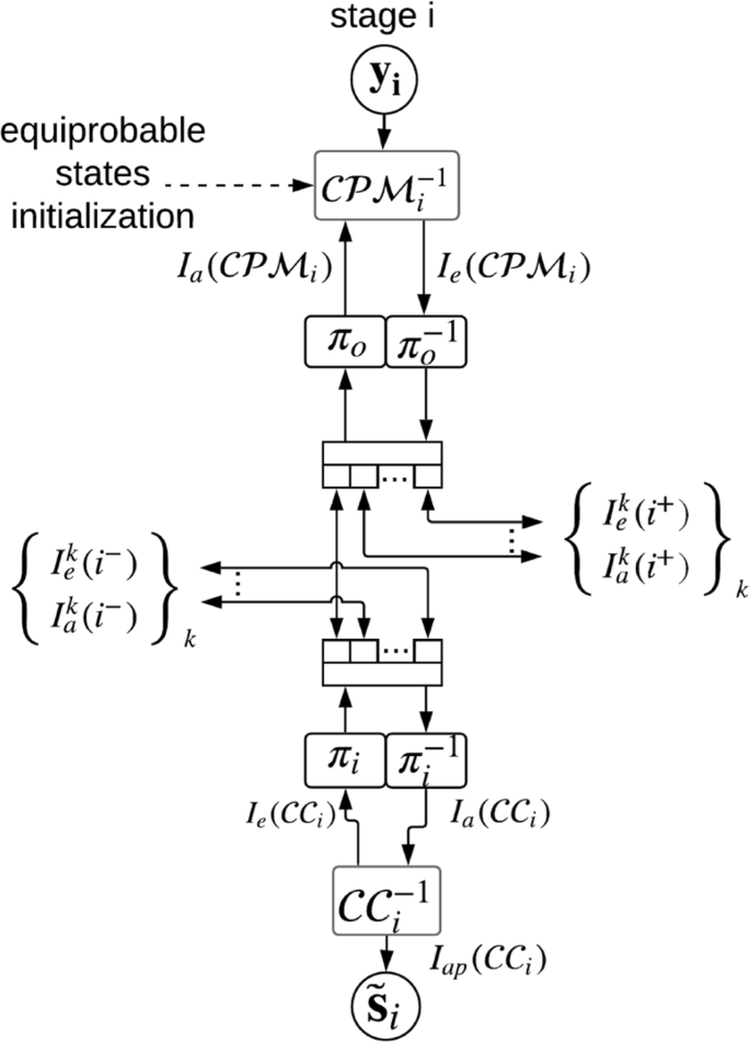

  

  The vectorized graph of the ith stage of the terminated SC-CPM receiver

• After deinterleaving, the mutual information of the bits and corresponding LLRs, shared from the stage i to the right-hand adjacent stage i+k, is given by $I_{e}^{k}(i^{+}) = I_{e}({\mathcal {C}\mathcal {P}\mathcal {M}}_{i}).b_{k}.$

• After a second deinterleaving, the a priori MI at the input of the outer decoder is given by the mixture $I_{a}({\mathcal {C}\mathcal {C}}_{i}) = \sum I_{a}^{k}(i^{-}).b_{k}$, where $I_{a}^{k}(i^{-})$ is the MI between the LLRs and corresponding bits shared from the left-hand adjacent stage i−k to the stage i. By convention, $I_{a}^{0}(i^{+}) = I_{e}({\mathcal {C}\mathcal {P}\mathcal {M}}_{i}).$

• The outer decoder then updates its extrinsic LLRs as $I_{e}({\mathcal {C}\mathcal {C}}_{i}) = T_{{\mathcal {C}\mathcal {C}}}(I_{a}({\mathcal {C}\mathcal {C}}_{i})).$

• After interleaving, the mutual information of the bits and corresponding LLRs, shared from the stage i to the left-hand adjacent stage i−k, is given by $I_{e}^{k}(i^{-}) = I_{e}({\mathcal {C}\mathcal {C}}_{i}).b_{k}.$

• After a second interleaving, the a priori MI at the input of the CPM demodulator is given by the mixture $I_{a}({\mathcal {C}\mathcal {P}\mathcal {M}}_{i}) = \sum I_{a}^{k}(i^{+}).b_{k}$, where $I_{a}^{k}(i^{+})$ is the MI between the LLRs and corresponding bits shared from the adjacent stage k+i to the stage i. By convention, $I_{a}^{0}(i^{+}) = I_{e}({\mathcal {C}\mathcal {C}}_{i}).$

• Wherever they are involved, the a priori MIs coming from the added padding bit nodes are taken equal to 1.

The threshold of the SC-CPM is then defined as the lowest channel noise parameter such that $I_{ap}({\mathcal {C}\mathcal {C}}_{i}) \rightarrow 1, \forall i$.

Note that the two concatenated interleavers π_i and π_o in Fig. 5 are here to ensure that the conducted asymptotic analysis depicts the average behavior of the system. In other words, when computing the different average mutual information $I_{a}({\mathcal {I}_{i})}$ and $I_{a}({\mathcal {O}_{i})}$, it is thanks to these two interleavers that we are able to write:

$$\begin{array}{*{20}l} I_{a}(\mathcal{I}_{i}) = \sum I_{a}^{k}(i^{+}).b_{k} \quad \text{and} \quad I_{a}(\mathcal{O}_{i}) = \sum I_{a}^{k}(i^{-}).b_{k} \end{array} $$

Without them, the computation of the threshold will refer to a particular family, corresponding to a particular realization of these two interleavers.

5.3 Coupling optimization

The asymptotic spatially coupled threshold described in the previous section suggests a large enough number of iterations. However, when designing practical turbo systems, speeding up the convergence rate is essential to minimize the decoding delay. With the coupling proposed in this paper, it is also possible to apply the optimization in [35] in order to reduce the decoding time without degrading the threshold. This is done as the following:

• 1 Draw an initial coupling matrix B. Several trials with different CPM schemes showed that the threshold of the SC-CPM corresponding to the uniform coupling matrix, b_k=1/(m_s+1), is a good representative of the SC-CPM ensemble threshold.

• 2 Applying the EXIT procedure described in the previous section, evaluate the threshold of the obtained SC-CPM.

• 3 Find another coupling matrix B such that the SC-CPM conserves the same threshold yet converges with a smaller number of iterations. Since this optimization problem is nonlinear, mainly due to the transfer functions $T_{{\mathcal {C}\mathcal {P}\mathcal {M}}(.)}$ and $T_{{\mathcal {C}\mathcal {C}}(.)}$, two optimization programming can be adopted:

  • (a) Greed search over a set of candidates of the form: $\left \lbrace \{b_{k}\}_{k} \vert \sum b_{k} = 1 \text { and } b_{k} \in \{\frac {a}{\Delta } \vert a \in [\!\![ 0, \Delta ]\!\!]\} \right \rbrace$, where $\Delta \in \mathbb {N}$ is a step constant

  • (b) Use the well-known differential evolution algorithm [42].

For both optimizations, the search space set can be extremely reduced by canceling symmetrical B. Further dimension reduction is achieved by replacing the equality constraint $\sum b_{k} = 1$ by the hyperplane $\sum _{i=0}^{m_{s}-1} b_{i} \leq 1$. Hence, the last component of B can be deduced until the end as $b_{m_{s}} = 1 - \sum _{i=0}^{m_{s}-1} b_{i}$.

6 Results and discussion

To illustrate the behavior and the performance of the proposed schemes, and without lake of generality, we first consider a serially concatenated coded CPM scheme using a systematic (5,7)₈ outer convolutional code concatenated with three different CPMs given as follows:

• A binary CPM scheme with parameters (L_c=1,h=1/2, Gaussian pulse);

• A quaternary CPM scheme with parameters (L_c=1,h=1/3, rectangular pulse, natural mapping);

• An octal CPM scheme with parameters (L_c=2,h=1/3, raised cosine pulse, natural mapping).

We first illustrate the spatial coupling gain using Fig. 7 and how it allows to improve the iterative decoding threshold of the underlying uncoupled serially concatenated system. In this figure, the evolution of the a posteriori MI, denoted as $I_{ap}({\mathcal {C}\mathcal {C}})$, associated with each replica/stage of the coupled chain is given for different numbers of iterations. L refers to the coupling length, i.e., the number of graph replicas. The x-axis refers to the spatial index l of one of the replicas in the coupled chain as illustrated in Fig. 5. This position index in the coupled chain is also equivalently denoted as stage position in the label of the figure. For a given colored curve with label number n, the y-axis gives the average a posteriori mutual information observed at the output of each of the lth iterative decoders after n iterations of the BP decoding process. Reaching the $I_{ap}({\mathcal {C}\mathcal {C}})=1$ at a given position means that the corresponding replica/stage has been correctly decoded. The threshold of the coupled ensemble is defined as the infimum of the E_s/N₀ values such that all replicas/stages converge to $I_{ap}({\mathcal {C}\mathcal {C}})=1.$ When iterative decoding fails, the decoding process is stopped at some indexes with $I_{ap}({\mathcal {C}\mathcal {C}})<1.$ This latter value is a function of the signal-to-noise ratio.

Fig. 7

Convergence of the binary SC-CPM stages as function of the decoding iterations (number above the lines) at E_s/N₀=−2.58 dB. Here, L=20

Thus, the different colored curves in Fig. 5 help to illustrate the classical double wave effect due to the coupling of the L replicas across iterations when the signal-to-noise ratio is above the convergence threshold of the coupled ensemble and how spatial coupling can help to improve iterative decoding performance. For our considered example, the threshold of the underlying uncoupled ensemble is E_s/N₀=−1.86 dB, meaning that it is unable to asymptotically achieve an arbitrary low probability of error for E_s/N₀ values below this threshold. However, we can observe that the coupled ensemble can converge at E_s/N₀=−2.58 dB. The rationale behind this phenomenon is that, thanks to the padding bits, the stages at the boundaries were able to converge, i.e, $I_{ap}({\mathcal {C}\mathcal {C}})$ tends to 1, at E_s/N₀=−2.58 dB. Then, thanks to the spatial coupling defined by the coupling matrix B, i.e, the linking between the different stages, reliable LLR values are shared to adjacent stages, which help these later to converge. This step-by-step convergence from the boundaries to the center of the SC-CPM propagates following a wave-like phenomenon, making the whole system to converge even at E_s/N₀=−2.58 dB. This improved threshold is due to the so-called coupling gain.

Figure 8 depicts the design rate R_L of the different schemes versus the corresponding BP thresholds when m_s=1 and B=[1/2,1/2]. These thresholds, referred to as “SC-CPM,” are the BP thresholds of the corresponding spatially coupled ensembles. As for the case of LDPC codes, it is conjectured to converge to the MAP threshold of the corresponding serially concatenated scheme as the coupling length L increases. This phenomenon is often referred to as threshold saturation. The performance of the coupled ensembles for different coupling lengths is compared to the following:

• The thresholds of the underlying uncoupled ensembles which are given by only one operating point, referred to as “coded CPM.” The obtained thresholds correspond to the BP thresholds of the uncoupled ensembles.

  Fig. 8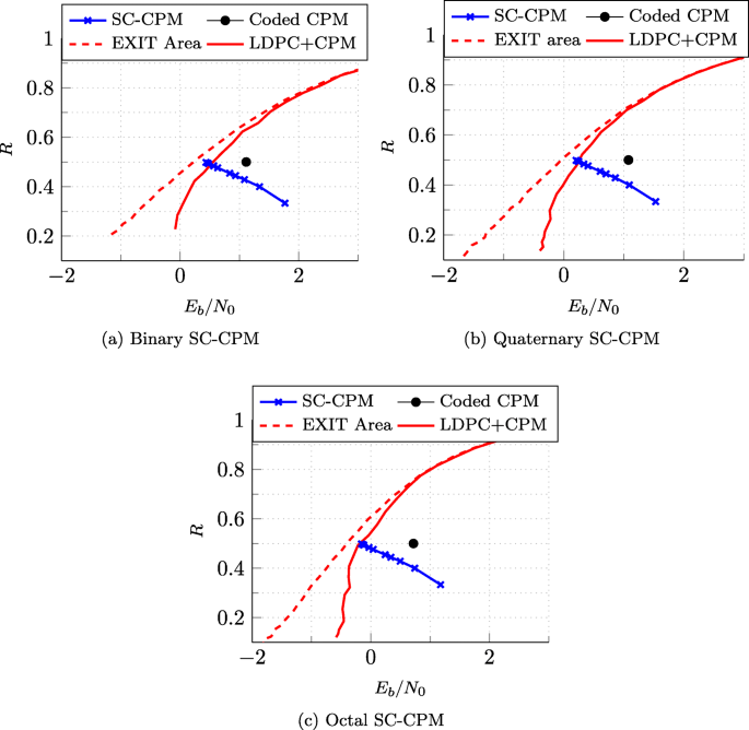

  

  Threshold of coupled and uncoupled coded CPM. Comparison to the area under the EXIT is also depicted. The coupling matrix here is $B=[\frac {1}{2}, \frac {1}{2}]$

• The maximum achievable rate for serially concatenated scheme using optimized LDPC codes [27], referred to as “LDPC+CPM.” The obtained thresholds correspond to the BP threshold under iterative detection and decoding.

• An estimation of the maximum achievable rate computed using the area under the EXIT curve, referred to as “EXIT area.” This curve is often conjectured to be a tight approximation of the normalized capacity associated with the inner detection scheme [37] (the inner CPM scheme in our context). It corresponds to an upper bound of the maximum achievable rate of any serially concatenated scheme involving the CPM scheme of interest.

For the binary CPM, spatial coupling allows to gain 0.68 dB in comparison to the uncoupled family and is at only 0.18 dB from the threshold given by the area theorem. Observe that this was achieved without any code design or optimization for the outer code. As L increases, the design rate R_L tends to 1/2 and the three SC-CPMs saturate to a value very close to the EXIT area theorem upper bound. This result corroborates the conjecture stating that the spatially coupled serially concatenated schemes saturate to a lower bound very close to the threshold given by the EXIT area theorem [35]. It is conjectured that it corresponds to the MAP threshold of the concatenated ensemble. This simply shows that, despite the limited performance of the uncoupled ensemble that does not operate close to the normalized capacity, very good thresholds can be achieved by spatial coupling for a scheme with a very regular structure. The same phenomenon has been observed for LDPC code ensembles for which it has been shown that spatial coupling of regular codes improves the BP threshold towards the MAP threshold that can be very close to the capacity. As a reference, we also plot the thresholds obtained by optimizing unstructured LDPC codes at different rates with maximum variable node degree of 7. We use the same optimization procedure as defined in [27] where both degree-1 variable nodes and their corresponding stability condition were considered. We observe that, for the three schemes, by coupling a simple (5,7)₈-coded CPM, we can reach or outperform the performance of the carefully designed serially concatenated coded CPM schemes using outer LDPC codes. Similar conclusions can be drawn from the two other subfigures corresponding to the quaternary and octal cases, respectively. Finally, Table 1 summarizes the thresholds of the considered schemes.

Table 1 Thresholds E_b/N₀ in decibel for different schemes at rates close to 1/2

The preceding results show how spatial coupling can help improve the iterative decoding threshold, even in the case of a very simple coupling. We now discuss the benefit of optimizing the coupling matrix. Figure 9 shows the number of iterations when uniform and optimized coupling matrices are used in the case of m_s=2. For the binary and the octal CPM schemes, we observe that the optimized schemes are able to converge around 17% and 13% faster than the uniform coupling matrix scheme. This has been observed in several other contexts. From this observation, we can conclude that optimizing the coupling structure does not necessarily improve the asymptotic threshold but rather help improve convergence speed.

Fig. 9

Iterations before convergence of different SC-CPM schemes with syndrome former memory m_s=2

For the special case of the CPM used in DVB-RCS2 standard [43], where h=1/5,L=2,α=1/3 and a natural mapping is used, we plot in Fig. 10 the obtained threshold computed for three schemes:

• 1 The serially concatenated scheme with an inner (5,7)₈ convolutional code

  Fig. 10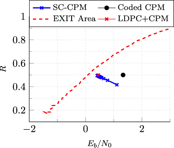

  

  Quaternary CPM used in DVB-RCS2 with h=1/5,L_c=2,α=1/3 and natural mapping. The coupling matrix is always given by $B=[\frac {1}{2}, \frac {1}{2}]$

• 2 The spatially coupled version of the previous scheme with respect to the coupling matrix B=[0.5,0.5]

• 3 The LDPC coded scheme with an optimized rate- 1/2 LDPC codes whose degree polynomials are given as: λ(x)=0.2006+0.6116x+0.1878x⁶ and ρ(x)=0.2x²+0.8x³

As we can see, the threshold of the SC-CPM scheme (i.e., 0.41 dB) outperforms the optimized LDPC code threshold (i.e., 0.45 dB). Both schemes 1 and 2 exhibit a coding gain of approximately 0.9 dB better that the DVB-RCS2 (5,7)₈-coded CPM scheme (whose threshold is at 1.33 dB).

Preceding results tend to show that performance of serially concatenated coded CPM schemes can be drastically improved by spatial coupling, pushing their performance very close to the maximum achievable rate, while the uncoupled ensemble exhibits limited performance. Remarkably, one is able to compete with state-of-art optimized LDPC coded solutions that are tailored for this application but with simple system components and a very regular structure, as it has been observed for regular LDPC codes. In general, as for the DVB-RCS2 context, any application that is considering concatenated schemes using CPMs such as in telemetry applications or tactical communications can be upgraded by considering a coupling strategy. The performance of such systems can be improved by coupling while each component of the emitter and the receiver (encoders and SISO decoders) can be reused from the initial setup and reassembled with a reasonable cost to enable coupling. Using an optimized coded CPM scheme with an outer LDPC code induces to change the complete layout of both the encoder and the decoder. Moreover, to achieve optimal performance, we cannot use on-the-shelf LDPC codes that are not efficient in this context. A specific design must be done, and the developed core may not be usable for any other application, since the design is dedicated to only one specific application.

7 Conclusion

In this paper, we proposed a method to spatially couple coded CPM schemes. Using an EXIT analysis, this scheme shows very competitive thresholds when compared to a carefully optimized LDPC code. Moreover, we introduced a design procedure to accelerate the convergence rate by optimizing the coupling matrix. Simulation results for different CPM schemes corroborate the conjecture that SC-CPM should also saturate to a value lower-bounded by the EXIT area theorem. Future work will investigate finite length performance and the optimization of the corresponding coupling base matrix.

References

J. B. Anderson, T. Aulin, C. -E. Sundberg, Digital phase modulation (Springer Science & Business Media, 1986).
B. E. Rimoldi, A decomposition approach to CPM. IEEE Trans. Inf. Theory. 34(2), 260–270 (1988).
M. Mouly, M. -B. Pautet, T. Foreword By-Haug, The GSM system for mobile communications (Telecom publishing, 1992).
M. Geoghegan, in 21st Century Military Communications Conference Proceedings MILCOM 2000, vol. 1. Description and performance results for a multi-h cpm telemetry waveform, (2000), pp. 353–357. https://doi.org/10.1109/milcom.2000.904974.
L. -J. Lampe, R. Tzschoppe, J. B. Huber, R. Schober, in IEEE International Conference on Communications, 2003. ICC’03, vol. 5. Noncoherent continuous-phase modulation for DS-CDMA, (2003), pp. 3282–3286. https://doi.org/10.1109/icc.2003.1204051.
T. F. Detwiler, Continuous phase modulation for high speed fiber optic links. PhD thesis, Georgia Institute of Technilogy (2011).
B. F. Beidas, S. Cioni, U. De Bie, A. Ginesi, R. Iyer-Seshadri, P. Kim, L. Lee, D. Oh, A. Noerpel, M. Papaleo, et al, Continuous phase modulation for broadband satellite communications: design and trade-offs. Int. J. Satell. Commun. Netw.31(5), 249–262 (2013).
M. K. Simon, Bandwidth-Efficient Digital Modulation with Application to Deep-Space Communications, vol. 2 (Wiley, 2005).
A. Scorzolini, V. De Perini, E. Razzano, G. Colavolpe, S. Mendes, P. Fiori, A. Sorbo, in Advanced Satellite Multimedia Systems Conference (ASMA) and the 11th Signal Processing for Space Communications Workshop (SPSC), 2010 5th. European enhanced space-based AIS system study, (2010), pp. 9–16. https://doi.org/10.1109/asms-spsc.2010.5586883.
Department of Defense Interface Standard. Interoperablility standard for single-acess 5-kHz and 25-kHz UHF satellite communications channels, in MIL-STD188-181B (USA Department of Defense, 1999).
Qualcomm, Waveform candidates. 3GPP TSG-RAN WG1, “R1-162199 (waveform candidates)”, 3GPP, 11–15 (2016).
X. Rui, Y. Huan, C. Qinglin, Adaptive coded modulation based on continuous phase modulation for inter-satellite links of global navigation satellite systems. IEEE Access (2018).
A. Barbieri, D. Fertonani, G. Colavolpe, Spectrally-efficient continuous phase modulations. IEEE Trans. Wirel. Commun.8(3), 1564–1572 (2009).
P. Moqvist, T. M. Aulin, in IEEE Trans. Commun., 49. Serially concatenated continuous phase modulation with iterative decoding, (2001), pp. 1901–1915.
K. R. Narayanan, G. L. Stuber, A serial concatenation approach to iterative demodulation and decoding. IEEE Trans. Commun.47(7), 956–961 (1999).
A. G. i Amat, C. A. Nour, C. Douillard, Serially concatenated continuous phase modulation for satellite communications. IEEE Trans. Wirel. Commun.8(6), 3260–3269 (2009).
C. Douillard, M. Jézéquel, C. Berrou, D. Electronique, A. Picart, P. Didier, A. Glavieux, Iterative correction of intersymbol interference: turbo-equalization. Eur. Trans. Telecommun.6(5), 507–511 (1995).
R. El Chall, F. Nouvel, M. Hélard, M. Liu, Iterative receivers combining mimo detection with turbo decoding: performance-complexity trade-offs. EURASIP J. Wirel. Commun. Netw.2015(1), 69 (2015).
S. K. Chronopoulos, V. Christofilakis, G. Tatsis, P. Kostarakis, Preliminary ber study of a tc-ofdm system operating under noisy conditions. J. Eng. Sci. Technol. Rev.9(4), 13–16 (2016).
S. K. Chronopoulos, V. Christofilakis, G. Tatsis, P. Kostarakis, Performance of turbo coded ofdm under the presence of various noise types. Wirel. Pers. Commun.87(4), 1319–1336 (2016).
K. R. Narayanan, I. Altunbas, R. Narayanaswami, in IEEE Global Telecommunications Conference (GLOBECOM), vol. 2. On the design of LDPC codes for MSK, (2001), pp. 1011–1015.
K. R. Narayanan, I. Altunbas, R. S. Narayanaswami, Design of serial concatenated msk schemes based on density evolution. IEEE Trans. Commun.51(8), 1283–1295 (2003).
A. Ganesan, Capacity estimation and code design principles for continuous phase modulation (CPM). PhD thesis, Texas A&M University (2003).
M. Xiao, T. M. Aulin, On analysis and design of low density generator matrix codes for continuous phase modulation. IEEE Trans. Wirel. Commun.6(9), 3440–3449 (2007).
M. Xiao, T. Aulin, Irregular repeat continuous phase modulation. IEEE Commun. Lett.9(8), 722–725 (2005).
T. Benaddi, C. Poulliat, M. -L. Boucheret, B. Gadat, G. Lesthievent, Design of systematic GIRA codes for CPM. Proc ISTC (2014). https://doi.org/10.1109/istc.2014.6955075.
T. Benaddi, C. Poulliat, M. -L. Boucheret, B. Gadat, G. Lesthievent, in 2014 IEEE International Symposium on Information Theory (ISIT). Design of unstructured and protograph-based LDPC coded continuous phase modulation, (2014), pp. 1982–1986. https://doi.org/10.1109/isit.2014.6875180.
T. Benaddi, C. Poulliat, M. -L. Boucheret, B. Gadat, G. Lesthievent, in IEEE International Conference on Communications, (ICC). Protograph-based LDPC convolutional codes for continuous phase modulation, (2014), pp. 1982–1986.
A. Jimenez Felstrom, K. S. Zigangirov, Time-varying periodic convolutional codes with low-density parity-check matrix. IEEE Trans. Inf. Theory. 45(6), 2181–2191 (1999).
D. G. Mitchell, M. Lentmaier, D. J. Costello, Spatially coupled LDPC codes constructed from protographs. IEEE Trans. Inf. Theory. 61(9), 4866–4889 (2015).
S. Kudekar, T. Richardson, R. Urbanke, Threshold saturation via spatial coupling: why convolutional LDPC ensembles perform so well over the BEC. IEEE Trans. Inf. Theory. 57(2), 803–834 (2011).
S. Moloudi, M. Lentmaier, A. G. i Amat, in 8th IEEE International Symposium on Turbo Codes and Iterative Information Processing (ISTC). Spatially coupled turbo codes, (2014), pp. 82–86.
S. Moloudi, M. Lentmaier, A. G. Amat, in International Symposium on Inf. Theory and Its Applications (ISITA). Finite length weight enumerator analysis of braided convolutional codes, (2016), pp. 488–492.
D. J. Costello, M. Lentmaier, D. G. Mitchell, in 9th International Symposium on Turbo Codes and Iterative Information Processing (ISTC), 2016. New perspectives on braided convolutional codes (IEEE, 2016), pp. 400–405. https://doi.org/10.1109/istc.2016.7593145.
T. Benaddi, C. Poulliat, R. Tajan, in GLOBECOM 2017-2017 IEEE Global Communications Conference. A general framework and optimization for spatially-coupled serially concatenated systems, (2017), pp. 1–6. https://doi.org/10.1109/glocom.2017.8254239.
G. Liva, Block codes based on sparse graphs for wireless communication systems. PhD thesis, University of Bologna (2006).
J. Hagenauer, in Proc. 12th European Signal Processing Conference (EUSIPCO). The exit chart-introduction to extrinsic information transfer in iterative processing, (2004), pp. 1541–1548.
L. Bahl, J. Cocke, F. Jelinek, J. Raviv, Optimal decoding of linear codes for minimizing symbol error rate (corresp.)IEEE Trans. Inf. Theory. 20:, 284–287 (1974).
P. Moqvist, T. Aulin, Trellis termination in CPM. Electron. Lett.36(23), 1940–1941 (2000).
T. Richardson, R. Urbanke, Modern coding theory (Cambridge University Press, 2008).
S. ten Brink, Convergence behavior of iteratively decoded parallel concatenated codes. IEEE Trans. Commun.49:, 1727–1737 (2001).
R. Storn, K. Price, Differential evolution–a simple and efficient heuristic for global optimization over continuous spaces. J. Glob. Optim.11(4), 341–359 (1997).
Second Generation DVB Interactive Satellite System (dvb-rcs2), in Digital Video Broadcasting (DVB), (2013).
Funding
Not applicable.
Author information
Authors and Affiliations
Contributions
TB is the main author of the current paper. TB contributed to the development of the ideas, design of the study, theory, result analysis, and article writing. CP contributed to the development of the ideas, design of the study, theory, result analysis, and article writing. The authors read and approved the final manuscript.
Corresponding author
Ethics declarations
Competing interests
Additional information
Publisher’s Note
Springer Nature remains neutral with regard to jurisdictional claims in published maps and institutional affiliations.
Rights and permissions
Open Access This article is licensed under a Creative Commons Attribution 4.0 International License, which permits use, sharing, adaptation, distribution and reproduction in any medium or format, as long as you give appropriate credit to the original author(s) and the source, provide a link to the Creative Commons licence, and indicate if changes were made. The images or other third party material in this article are included in the article’s Creative Commons licence, unless indicated otherwise in a credit line to the material. If material is not included in the article’s Creative Commons licence and your intended use is not permitted by statutory regulation or exceeds the permitted use, you will need to obtain permission directly from the copyright holder. To view a copy of this licence, visit http://creativecommons.org/licenses/by/4.0/.
About this article
Cite this article
Benaddi, T., Poulliat, C. Spatially coupled turbo-coded continuous phase modulation: asymptotic analysis and optimization. J Wireless Com Network 2020, 159 (2020). https://doi.org/10.1186/s13638-020-01773-7
Received:
Accepted:
Published:
DOI: https://doi.org/10.1186/s13638-020-01773-7