Experimental evaluation of flexible duplexing in multi-tier MIMO networks

Abstract

In this paper, we present an experimental evaluation of the performance benefits provided by flexible duplexing, an access technique that allows uplink and downlink cells to coexist within the same time-frequency resource blocks. In order to replicate a wireless multi-tier network composed of 1 macro-cell and 2 small cells, a measurement campaign has been conducted using an indoor wireless testbed comprised of a total of 6 multiple-input multiple-output (MIMO) software-defined radio (SDR) devices. Since each cell has a single active user, each uplink/downlink configuration can be identified with a different interference channel, over which interference alignment (IA) is used as an inter-cell interference management technique and compared to other existing methods. The obtained results show that flexible duplexing clearly outperforms the conventional time-division duplex (TDD) access approach, where all cells operate synchronized either in uplink or dowlink mode. Additionally, interference alignment consistently provides better results in most of the interference regimes when compared to minimum mean square error (MMSE)-based schemes. The impact of channel estimate quality on the different communication strategies is also studied. It is worth highlighting that the presented over-the-air (OTA) experiments represent the first implementation of IA with real-time precoding and decoding.

1 Introduction

Motivated by the deployment of multiple-input multiple-output (MIMO) heterogeneous networks (HetNets) [1], flexible duplexing has arisen as a promising access technique in the context of 5G communications. The main idea behind this approach consists in allowing the coexistence of uplink (UL) and downlink (DL) cells in the same resource blocks, i.e., within the same time and frequency slots. Each UL/DL configuration generates a different interference level at the input of the receivers, hence affecting the quality of service (QoS). Nevertheless, advanced interference management (IM) techniques, such as interference alignment (IA), or more conventional techniques such as minimum mean square error (MMSE)-based decoding, still need to be applied in combination with flexible duplexing in order to mitigate both intra-cell and inter-cell interference appropriately.

Flexible duplexing was initially proposed under the name of reverse time-division duplex (R-TDD) [2] or dynamic-TDD [3], and over the last years, a number of theoretical studies have been carried out. Authors in [4] analyze the degrees of freedom (DoF) benefits of flexible duplexing in 2-cell networks by combining reversed UL/DL with interference alignment. The DoF study is extended for multi-cell networks in [5], where the impact of network asymmetry on the potential multiplexing gain is discussed. First results showing the rate improvements provided by flexible duplexing can be found in [2]. Furthermore, a reverse-TDD scheme is introduced in [6] in the context of massive MIMO HetNets with dense small-cell tiers, providing additional results in terms of increased coverage probability and spectral efficiency. Afterwards, flexible duplexing is applied to dense HetNets with wireless backhaul in [7], and a joint user scheduling, precoding, and UL/DL selection framework is presented in [8]. Also, the aforementioned work takes into account traffic asymmetries for a better characterization of 5G mobile communications. Such asymmetries are included as well in [9], where following the same line as in [4, 5], flexible duplexing is combined with IA for optimal downlink rate. In addition, the hierarchical switching (HS) scheme, which checks only a subset of possible uplink/downlink configurations, is proposed in order to reduce the computational cost of UL/DL selection.

Additionally, remarkable advances have been made regarding power efficiency by means of flexible duplexing. Specifically, a power optimization method with flexible UL/DL sets and full-duplex base stations (BS) is presented in [10]. Afterwards, authors in [11] analyzed the coexistence of UL and DL cells in terms of downlink transmit power. A deeper study is performed in [12], where authors introduce a variation of flexible duplexing called α-duplex. In this model, a partial bandwidth overlap is allowed among uplink and downlink frequency-division duplex (FDD) slots, and the data rate is optimized subject to power constraints, so as to determine user scheduling as well. Finally, a power minimization algorithm is proposed in [13] to optimize the total transmit power for a given UL/DL combination, and then combined with the HS approach in [9] to select the best duplexing configuration.

1.1 Contributions

In this work, we go a step further and evaluate the potential benefits of flexible duplexing through a set of over-the-air (OTA) experiments that try to reproduce a multi-tier MIMO network. We distinguish two levels of study. On the one hand, we compare flexible duplexing to conventional TDD. On the other hand, we analyze the performance of flexible duplexing in combination with different inter-cell IM techniques. The rest of the paper is organized as follows: first, we present the multi-cell network topology. We then provide a brief introduction of the considered IM techniques with an emphasis on the concept of IA, together with a discussion on the main practical difficulties related to IA implementations. Once the main challenges have been described, we present the experimental setup on which we have conducted the measurement campaign. Finally, the experimental results are shown and analyzed in detail. It is worth mentioning that, despite real-time blind IA (BIA) experiments which can be found in [14, 15], this work is the first implementation of IA with both global channel state information (CSI) and real-time precoding and decoding at all nodes in the network.

2 Network model and interference management techniques

The considered scenario comprises 2 tiers, including G_m macrocells and G_s small cells with G=G_m+G_s cells. Each cell $g\in \left \{1,2,\dots,G\right \}$ has an $N_{BS_{g}}$-antenna base station (macro-tier), or $N_{AP_{g}}$-antenna access point (small tier), and user equipments with $N_{UE_{g}}$ antennas. There is a single orthogonal frequency-division multiplexing (OFDM) stream per user, and the intra-cell interference is assumed to be handled by means of resource block scheduling. Therefore, a single active user per cell is considered.

In such network, and assuming that a linear precoding/decoding technique is applied, the received signal at the input of receiver g is expressed by

$$\begin{array}{*{20}l} r_{g} &= u_{g}^{H}\mathbf{n}_{g} + i_{g}\mathbf{u}_{g}^{H}d_{gg}^{-\alpha/2}\mathbf{H}_{gg}P_{BA_{g}}^{1/2}\mathbf{v}_{g}s_{g} + \left(1-i_{g}\right)\mathbf{u}_{g}^{H}d_{gg}^{-\alpha/2}\mathbf{H}_{gg}P_{UE_{g}}^{1/2}\mathbf{v}_{g}s_{g} \notag \\ &+\sum_{j=1,j\neq g}^{G}\left(i_{j}\mathbf{u}_{g}^{H}d_{gj}^{-\alpha/2}\mathbf{H}_{gj}P_{BA_{j}}^{1/2}\mathbf{v}_{j}s_{j} + \left(1-i_{j}\right)\mathbf{u}_{g}^{H}d_{gj}^{-\alpha/2}\mathbf{H}_{gj}P_{UE_{j}}^{1/2}\mathbf{v}_{j}s_{j}\right) \quad\forall g \end{array} $$

(1)

where i_g is a Boolean variable indicating whether each cell g is in downlink (i_g=1) or in uplink (i_g=0), and s_g contains the information that transmitter g is sending to receiver g. H_gj is the MIMO channel from transmitter j to receiver g, and n_g is the noise at receiver g. Also, $P_{BA_{g}}$ is the power level at the BS (AP) of macro (small) cell g, $P_{UE_{g}}$ is the power level at the gth UE, and d_gj is the normalized distance from the jth transmitter to receiver g, whereas α denotes path loss exponent. Finally, v_g and u_g are the precoding and decoding vectors (i.e., beamformers) applied at transmitter and receiver g, respectively¹.

As shown in Fig. 1, the scenario under evaluation contains G=3 cells with 1 macrocell and 2 small cells, where each cell includes a single active user. All the nodes in the network are equipped with 2 antennas, and as above mentioned, there is a single (OFDM) stream per cell. Therefore, according to the convention in [16], we are working with a set of multi-carrier (2×2,1)³ interference channels (IC), each one associated to a different UL/DL combination. Consequently, for any given UL/DL setting, the signal model in (1) can be reformulated as

$$ \mathbf{r}_{g} = \mathbf{u}_{g}^{H}\left(d_{gg}^{-\alpha/2}\mathbf{H}_{gg}P_{g}\mathbf{v}_{g}s_{g} + \sum_{j\neq g}^{G}d_{gj}^{-\alpha/2}\mathbf{H}_{gj}P_{j}\mathbf{v}_{j}s_{j} + \mathbf{n}_{g}\right)\quad\forall g, $$

(2)

Fig. 1

Multi-tier network topology under evaluation

where $P_{g} = i_{g}P_{BA_{g}} + \left (1-i_{g}\right)P_{UE_{g}}$ is the power level at transmitter g∈{1,2,3}.

In order to characterize the impact of flexible duplexing on the network performance, we compare three different interference management strategies. Two of these techniques are based on multi-cell minimum mean square error (M-MMSE) receivers and will be described in Section 2.1. Analogously, the IA scheme is introduced in Section 2.2.

2.1 Multi-cell MMSE

The M-MMSE technique [17, 18], also called interference rejection combining (IRC) in the literature [19], is an extension of the well-known MMSE technique that takes into account the knowledge of the channels from interferers to the intended receiver g, i.e. $\{\mathbf {H}_{gj}\}_{j\neq g}^{G}$. From (2), the M-MMSE filter at a given user g, $\mathbf {u}_{g}^{\mathrm {M-MMSE}}$, is calculated as

$$ \mathbf{u}_{g}^{\mathrm{M-MMSE}} = \mathbf{v}_{g}^{H}\hat{\mathbf{H}}_{gg}^{H}\left(\hat{\mathbf{H}}_{gg}\mathbf{v}_{g} P_{g}d_{gg}^{-\alpha}\mathbf{v}_{g}^{H}\hat{\mathbf{H}}_{gg}^{H}+\mathbf{R}_{g}+\mathbf{n}_{g}\right)^{-1}\quad\forall g, $$

(3)

where, $\mathbf {R}_{g} = \sum _{j\neq g}^{G}\hat {\mathbf {H}}_{gj}\mathbf {v}_{j} P_{j}d_{gj}^{-\alpha }\mathbf {v}_{j}^{H}\hat {\mathbf {H}}_{gj}^{H}$ is the covariance matrix of the inter-cell interference, and $\hat {\mathbf {H}}_{gj}$ is the estimated channel matrix between transmitter j and receiver g.

At the transmitter side, two different strategies are considered to calculate the beamforming vectors:

• Complex random unit norm precoders, in such a way that a sufficient number of transmissions is statistically equivalent to an isotropic spatial distribution.

• Dominant eigenmode transmission (DET), i.e., the precoder is the eigenvector associated to the maximum eigenvalue of the channel matrix between the transmitter and the intended receiver.

2.2 Spatial interference alignment

The main intuition behind the interference alignment technique is to confine interfering signals into a reduced dimensionality subspace at each receiver, allowing us to transmit the desired signals simultaneously over the remaining interference-free subspace [20]. Although, multiple time and frequency dimensions can be exploited, we focus on the spatial dimension in our implementation.

Spatial IA builds on a set of precoders $\{\mathbf {v}_{g}\}_{g=1}^{G}$ and decoders $\{\mathbf {u}_{g}\}_{g=1}^{G}$, that must fulfill the following conditions for all transmitter-receiver pairs²,

$$ \left\{\begin{array}{ll} \mathbf{u}_{g}^{H} \mathbf{H}_{gg} \mathbf{v}_{g} \neq 0 &\forall g \\ \mathbf{u}_{g}^{H}\mathbf{H}_{gj} \mathbf{v}_{j}=0,&\forall j\neq g. \end{array}\right. $$

(4)

Several IA algorithms are available in the existing literature for more general interference channels [21–23], as well as for more sophisticated topologies [24]. Nevertheless, for the (2×2,1)³ interference channel under evaluation, an analytical procedure to calculate the beamformers and filters satisfying (4) was proposed in [20]:

• 1. The precoder for user 1, v₁, can be selected as any eigenvector of matrix

  $$\mathbf{E} = \left(\mathbf{H}_{31}\right)^{-1}\mathbf{H}_{32}\left(\mathbf{H}_{12}\right)^{-1}\mathbf{H}_{13}\left(\mathbf{H}_{23}\right)^{-1}\mathbf{H}_{21}. $$

• 2. From v₁, precoders v₂ and v₃ can be calculated as

  $$\mathbf{v}_{2} = \left(\mathbf{H}_{32}\right)^{-1}\mathbf{H}_{31}\mathbf{v}_{1} $$
  $$\mathbf{v}_{3} = \left(\mathbf{H}_{23}\right)^{-1}\mathbf{H}_{21}\mathbf{v}_{1} $$

• 3. The interference cancelation filters must be designed in such a way that the received signal is projected on the orthogonal subspace of the interference signal space. Equivalently, u₁ is the eigenvector of [H₁₂v₂ H₁₃v₃] associated to the zero eigenvalue, whereas u₂ and u₃ can be obtained analogously from [H₂₁v₁ H₂₃v₃] and [H₃₁v₁ H₃₂v₂].

As previously discussed in [25], several impairments can be found when IA is implemented in practice, limiting its performance when compared to the theoretical results:

• While perfect channel knowledge is assumed in theory, channel estimation errors arise in practice. The impact of the resulting misalignment is taken into account for the theoretical studies in [9, 26], as well as in the experiments discussed in [27, 28].

• Spatial collinearity between desired signal and interference subspaces could result in desired signal energy loss.

• IA precoders and decoders are usually applied at symbol level in a per-subcarrier fashion, i.e., after frame detection and time/frequency synchronization stages. However, in real-world systems, detection and synchronization are performed right after the RF demodulation and analog-to-digital conversion, i.e., at sample level, thus they are affected by interference. The pre-FFT IA approach in [29, 30] overcomes this issue by operating at sample level, that is, in the time domain. Nevertheless, since the synchronization mismatches have been already studied in the aforementioned works, we rely on an external clock and oscillator for time and frequency synchronization (see Section 3), and apply IA precoders and decoders in the frequency domain.

3 Multiuser MIMO testbed

After going through the main challenges that can arise when implementing interference alignment, we provide a detailed description of the experimental setup that we have built in order to study the benefits of applying flexible duplexing. The MIMO HetNet that we have implemented is based on Ettus Universal Software Radio Peripheral (USRP) devices. Specifically, each node in the network is associated to a 2-antenna USRP B210, equipped with an Analog Devices AD9361 RF frontend and a Xilinx Spartan 6 XC6SLX150 field-programmable gate array (FPGA). These transceivers are capable of both up and down conversion ranging from 70 MHz up to 6 GHz with a maximum instantaneous bandwidth of 30.72 MHz³. Therefore, B210 boards are conveniently suitable for experiments in the 2.4 GHz industrial, scientific, and medical (ISM) radio band.

Even though several practical mismatches could impair the measurements as explained in Section 2.2, most of them have been studied in previous works, while for this campaign, we wish to analyze the benefits of flexible duplexing isolatedly. For this reason, we rely on an Ettus OctoClock-G external reference, connected to all the nodes through calibrated coaxial cables, in order to guarantee time and frequency synchronization. More specifically, pulse-per-second (PPS) and 10 MHz reference signals are sent to the B210 to avoid frequency offsets and/or frame detection misalignments throughout the measurement procedures.

Additionally, the boards are connected to high-performance PC hosts, in such a way that we can configure the elements in the network, write the signals to be transmitted by the corresponding transmitters, and retrieve the signals at the receivers. For this purpose, we have relied on the source code of the GTEC Testbed developed at the University of A Coruña⁴. This package provides an interface between MATLAB code and the UHD/GNU Radio libraries, so that the different devices in the experiment can be configured and controlled in a flexible way. Also, the nodes connected to the PC hosts can be accessed either locally or remotely, allowing to perform the measurements remotely and synchronously, i.e., the time instants at which transmitters send their frames over the air and the time instants at which the receivers acquire those frames are defined beforehand directly from MATLAB code. Figure 2 shows the basic scheme for a 2×2 MIMO link, including transmitting and receiving USRP B210 boards, PC hosts, and the Octoclock device that guarantees time and frequency synchronization between the nodes.

Fig. 2

Hardware scheme for a 2×2 point-to-point link

4 Experimental setup

Figure 3 displays the 3-cell network in which the experiments have been conducted. As mentioned above, the setup is comprised of a macro base station (BS1) with its corresponding user equipment (MUE1), as well as two small access points (AP2 and AP3), each one serving a single user equipment (SUE2 and SUE3, respectively). All these elements are connected to the same Octoclock-G device, which provides the required time and frequency external references. It is worth mentioning that the cables between the Octoclock and the B210 boards have equal length in order to preserve the accuracy of the reference signals among different users. As presented in Fig. 3, the configuration is intended to emulate a network where the UEs and the small-cell APs coexist in a small area, being one of the UEs served by a macro BS. All the aforementioned unities are equipped with 2 antennas, with a self-inter-antenna distance of 66 millimeters given by the separation between the antenna ports in the USRP device. Moreover, the distances between the different nodes in Fig. 3 is included in Table 1. In practice, the influence of the different distances in the scenario under evaluation is taken into account implicitly within the corresponding channel estimates.

Fig. 3

Experimental 3-cell setup at the GTAS laboratory

Table 1 Distance between every pair of nodes in the network (meters)

Regarding the signals to be sent over the air, we have defined the frames in Fig. 5 as a variation of the IEEE 802.11a physical layer frame format. The OFDM frames have been transmitted at a center frequency of 2.487 GHz and 1 MHz bandwidth (including guard subcarriers). Since the different transmission strategies to be assessed should experiment similar channel realizations for the sake of a fair comparison, we have checked that the indoor channel in the laboratory remains invariant for a number of OFDM symbols (see Fig. 4).

Fig. 4

Indoor channel in the GTAS laboratory at a center frequency of 2.487 GHz

Fig. 5

Frame structure for each user in the network, where 0 means no signal transmission for the given time slot or antenna

As in the case of 802.11a, each frame includes a total of 52 subcarriers (64-point FFT), 48 of which convey data symbols. The frame headers comprise the conventional short-training symbols (ST) for frame detection purposes, as well as long-training symbols (LT) allowing to correct slight frequency offsets in settings with no frequency synchronization. The signal field (SF) has been included in the frame format as specified in the 802.11a PHY-layer specification, despite no rate adaptation being performed throughout the measurement campaign. Additionally, in order to estimate all the single-input single-output (SISO) channels between each antenna pair within the 3-cell network, we have modified the frame header by adding a structured sequence of long-training symbols and zero-padding. The format described above is depicted in Fig. 5. Finally, a total of 21 OFDM data symbols are transmitted within each frame, in order to compare the three different interference management strategies, namely:

• Interference alignment

• DET transmission + M-MMSE reception

• Random precoding + M-MMSE reception

For all three techniques, each data subcarrier includes QPSK symbols, yielding a total of 2016 bits per frame.

5 Measurement methodology

The relevance of the results rely on a well-designed measurement procedure. In this section, we describe the main steps that we have performed throughout the experiments. First, for a given UL/DL combination, the following steps are performed:

• 1 Initial channel estimate: For the first transmission, no channel knowledge is available. Therefore, an initialization frame with no relevant data symbols is transmitted in order to obtain the first channel estimate⁵.

• 2 Precoder/decoder design: Once we have estimates of the desired and interfering channels, we obtain the IA precoders and decoders, and the DET precoders. This step is performed by means of a centralized calculation at the PC hosts, and the precoding and decoding vectors are obtained in the frequency domain, i.e., on a per-subcarrier basis.

• 3 Data transmission: For each frame and user, 7 IA-precoded OFDM symbols are included, followed by 7 DET-precoded symbols and 7 symbols transmitted with randomly generated precoders.

• 4 Channel estimate and real-time symbol decoding: Once the transmitted frames are detected at the receivers, the CSI is updated and the M-MMSE filters are calculated. The IA decoders are applied to the first 7 data symbols, and the remaining 14 are M-MMSE decoded. With the new channel estimate, IA precoders and decoders, as well as DET precoders, are calculated for the next transmission, or equivalently, the procedure continues back at step 2.

Unlike the first frame, which is sent without any previous channel knowledge, the precoders and decoders corresponding to the nth frame can be calculated with the channel estimate obtained from the previous frame n−1. This way, there is no need for including training-only frames before each data transmission, improving the efficiency of the experimental procedure.

For each experiment, the error vector magnitude (EVM) for the received symbols is calculated as

$$ \text{EVM}_{s} = \frac{\sum_{n}\left|\hat{z}_{s,n}-z_{s,n}\right|^{2}}{\sum_{n}\left|z_{s,n}\right|^{2}}, $$

(5)

where s is the subcarrier index, n is the OFDM data symbol index, z_s,n is the originally transmitted symbol and $\hat {z}_{s,n}$ is the decoded symbol at the receiver. Finally, the median EVM for the symbols decoded with the three considered schemes is obtained. The reason for considering the median is that, throughout the measurement campaign, a sparse amount of frames might be affected by external perturbations. Despite being a reduced number of cases, these outliers have a significant impact on the mean EVM. After checking that the probability density function (PDF) of the EVM is approximately symmetric around its mean (without considering the erroneous realizations), we can assume that the median is a sufficiently accurate approximation for the mean EVM.

Finally, it is worth mentioning that other figures of merit for system performance have not been taken into account for the following reasons:

• As described in Section 4, the throughput in the considered scenario is constant. Specifically, QPSK symbols are transmitted over 52 (48 data) subcarriers with a total bandwidth of 1 MHz. Even if rate adaptation is applied as in IEEE 802.11 standards, there would be still a discrete set of rates (e.g., 54/48/36/24/12/9/6 megabits per second in IEEE 802.11a); thus, a continuous characterization of performance in terms of such metric would not be accurate. Also, notice that implementing rate adaptation in our setup, which requires additional feedback from receivers to transmitters, would shift the focus away from the actual interference management techniques under evaluation.

• While EVM provides a continuous measure of how close a received symbol is to the transmitted symbol, bit errors provide a binary indicator regarding successful/missed decoding. Furthermore, for a statistically sufficient number of bit errors to occur in the considered setup, an extremely large amount of transmissions would be required. For these reasons, bit error rate (BER) has been discarded as a figure of merit in this work.

6 Experimental results and discussion

In this campaign, we assess the performance of flexible duplexing in the setup described in Section 4 for different UL/DL combinations within a range of interference regimes. For this purpose, we have fixed the transmit power at the APs to −31 dBm and at the UEs to −34 dBm in the small cells⁶. The steps described in Section 5 are repeated for several transmit power levels at the downlink macro BS and different UL/DL configurations in the small cells. In other words, we analyze the impact of inter-cell interference coming from the macrocell onto the different small cells and how selecting the best UL/DL combination mitigates such impact. Specifically, 100 frames are transmitted by each node for each BS transmit power value. Further, the EVM versus the BS transmit power is obtained in such a way that different UL/DL settings can be compared, including the conventional TDD approach. It is worth mentioning that, for the sake of neatness and clarity, we provide a selection of the most significant results. Throughout our measurement campaign, we have observed that flexible duplexing provides the highest improvement rates in the case of small cell user equipments (SUE 2 and SUE 3). For this reason, we display the following results:

• Median EVM at MUE 1 for the three schemes under test in [DL UL UL] mode

• Median EVM at SUE 2 for the three schemes under test in [DL DL UL] mode

• Median EVM at MUE 3 for the three schemes under test in [DL UL DL] mode

• Median EVM degradation at SUE 3 for the three schemes under test in conventional TDD ([DL DL DL]) mode with respect to [DL UL DL] mode

The median EVM obtained at MUE 1 by the three IM schemes under comparison is shown in Fig. 6 for the setting [DL UL UL]. In other words, the macrocell is in downlink whereas both small cells are in uplink. Lower transmit power levels at the BS translate into a lower desired signal quality at the MUE 1 in the macrocell. Consequently, the lower signal-to-interference-plus-noise ratio (SINR) provokes higher EVM for all the communication strategies under evaluation. On the contrary, the SINR increases for higher power levels at the macrocell, hence improving the EVM results at MUE 1. As expected, IA provides the best performance out of the three techniques, while M-MMSE is slightly outperformed by DET+M-MMSE as well. Notice that IA precoders and decoders are specifically designed to suppress the interference at the unintended receivers. On the other hand, the M-MMSE techniques simply aim to minimize the error at the receiver; thus, they take no advantage from any knowledge about the interfering signals.

Fig. 6

Median EVM at MUE 1 for the three schemes under test in [DL UL UL] mode

Figures 7 and 8, respectively, show the results at SUE 2 and SUE 3 for different UL/DL combinations. In this case, the macrocell is in downlink mode, one of the small cells is in uplink, and the other small cell is in downlink, i.e., [DL DL UL] or [DL UL DL]. The main difference when focusing on the small cells is that, unlike the previous case, an increase in the transmit power at the macro BS implies a higher inter-cell interference. Therefore, as the BS power level increases, the SINR at the small cells decreases, hence compromising the EVM. From Fig. 8, we can distinguish two different regimes, namely,

• From −40 to −35 dBm BS transmit power,M-MMSE with random precoding is, surprisingly, the best out of the three communication schemes. The main reason for this is the quality of the channel estimates. Specifically, even though channel estimation tasks are carried out in a time-division multiple access (TDMA) fashion, thus free of interference, the signal-to-noise ratio (SNR) of the training symbols is lower for low transmit power regimes at the BS. The impact of such impairment is less significant for M-MMSE, which requires CSI at the receivers only. On the contrary, each user applying DET+M-MMSE requires the channel estimates from its own transmitter to all receivers, both at the transmitter and receiver ends. Additionally, IA requires global CSI knowledge, hence being the most penalized technique.

  Fig. 7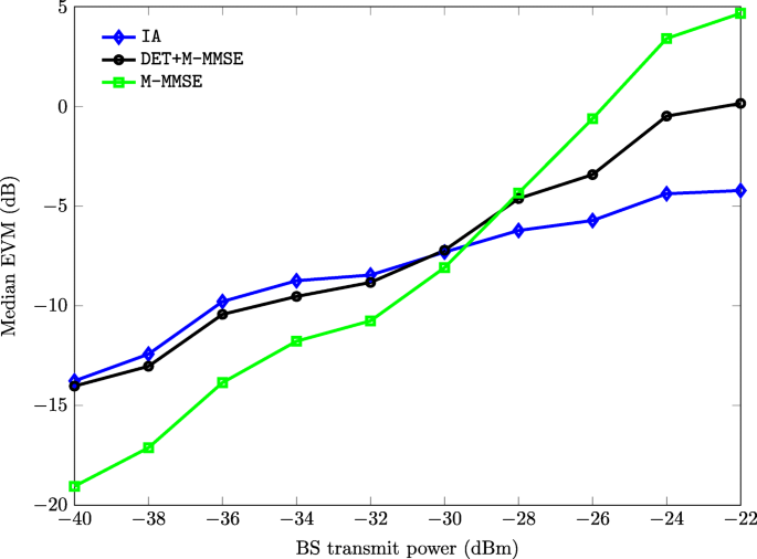

  

  Median EVM at SUE 2 for the three schemes under test in [DL DL UL] mode

  Fig. 8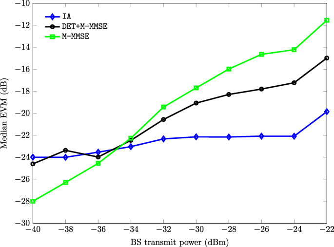

  

  Median EVM at SUE 3 for the three schemes under test in [DL UL DL] mode

• From −35 to −22 dBm BS transmit power, the SNR for channel estimation increases, and therefore, the quality of the estimates is improved. In this situation, the beamforming-based techniques take full advantage of their channel knowledge and outperform M-MMSE. We can state that IA provides the best results in this regime, maintaining a remarkable performance even when the interfering signal strength is higher than that of the desired signal. Recall that transmit power for AP at the small cells is −31 dBm, whereas the BS at the macrocell is transmitting up to −22 dBm.

Above −22 dBm, and with the spatial location of the nodes in the network, the power at the BS is high enough to saturate the input of the receivers. Recall that, although base stations in real deployments transmit much higher power levels, our evaluation has been carried out for a small-scale representation in an indoor environment. The different transmit power levels have been accordingly adapted to the dynamic range of the receivers.

Once we have studied the different precoding/decoding methods, we focus on the performance benefits that flexible duplexing provides when compared to conventional TDD configurations. For this purpose, Fig. 9 shows the EVM degradation suffered at SUE 3 in conventional TDD mode with respect to the best UL/DL combination previously presented in Fig. 8. Flexible duplexing clearly outperforms conventional TDD regardless of the interference management technique applied at the transmitters and receivers. Nevertheless, different improvement levels can be quantified for the different strategies. Despite IA being the scheme with the best performance in the experiments, the M-MMSE-based methods are more benefited by selecting the UL/DL combination with the lowest interference level at the receivers.

Fig. 9

Median EVM degradation at SUE 3 for the three schemes under test in conventional TDD mode with respect to [DL UL DL] mode

The main intuition behind this result is that, IA being specifically designed to suppress the interference at the unintended receivers, a consistent performance is provided regardless of the UL/DL configuration in the network. For ideal scenarios, indeed, the particular configuration determined by the flexible duplexing technique may cause no difference when implementing IA. However, the practical impairments given in real-world scenarios, such as channel estimation errors or different spatial distributions, provoke different interference leakage levels depending on the UL/DL setting. For this reason, improvements up to 3 dB have been achieved by selecting the appropriate configuration.

On the other hand, DET+M-MMSE and M-MMSE are not specifically intended to handle the interfering signals; thus, residual interference remains even under ideal conditions. Practical misalignments emphasize such interference leakage and hence a selection of the best UL/DL mode is crucial, especially in the case of M-MMSE. Benefits up to 10 dB can be attained for low-SINR regimes, as observed in Fig. 9. Recall that beamforming-based techniques, in this case IA and DET+M-MMSE, use the multiple antennas at the transmitter to radiate the transmitted power along a specific spatial direction, thus having a reduced impact on other receivers. To some extent, we could state that flexible duplexing has less room for improvement in such cases. However, M-MMSE takes full advantage of flexible duplexing since the different UL/DL combinations are the only factor making a difference in terms of interference at the receivers.

7 Conclusion

Flexible duplexing has been experimentally evaluated in a small-scale deployment with high-performance devices. The presented experiments have also served to test the applicability of interference alignment in realistic environments. For this reason, we have provided a brief review on the most remarkable advances regarding IA experiments, as well as on a number of practical impairments that arise when IA is applied in real-world scenarios. After settling the background, we have conducted our experimental study on two different levels. On the one hand, we have compared flexible duplexing and conventional TDD. The empirical results corroborate the conclusions achieved in the existing literature, since a noticeable improvement is achieved by means of flexible UL/DL combining over standard TDD. On the other hand, we have compared interference alignment to other well-known transmission techniques, namely M-MMSE and DET+M-MMSE. Even though IA is considerably affected by practical impairments, such as channel estimation errors, it outperforms the other communication schemes under test. It is especially worth mentioning that our experiment has represented the first real-time implementation of IA with global CSI and on-line precoding and decoding.

References

X. Chu, D. L. Perez, Y. Yang, F. Gunnarsson, Heterogeneous cellular networks: theory, simulation and deployment (Cambridge University Press, New York, 2013).
J. Hoydis, K. Hosseini, S. t. Brink, M. Debbah, Making smart use of excess antennas: massive MIMO, small cells, and TDD. Bell Labs Tech. J.18(2), 5–21 (2013). https://doi.org/10.1002/bltj.21602.
J. Kerttula, A. Marttinen, K. Ruttik, R. Jäntti, M. N. Alam, Dynamic TDD in LTE small cells. EURASIP J. Wirel. Commun. Netw.2016(1) (2016). https://doi.org/10.1186/s13638-016-0696-z.
S. -W. Jeon, K. Kim, J. Yang, D. K. Kim, The feasibility of interference alignment for MIMO interfering broadcast-multiple-access channels. IEEE Trans. Wirel. Commun.16(7), 4614–4625 (2017). https://doi.org/10.1109/TWC.2017.2700465.
J. Fanjul, I. Santamaria, in 24th European Signal Processing Conference (EUSIPCO). On the spatial degrees of freedom benefits of reverse TDD in multicell MIMO networks, (2016). https://doi.org/10.1109/eusipco.2016.7760471.
M. Kountouris, N. Pappas, in 2013 IEEE-APS Topical Conference on Antennas and Propagation in Wireless Communications (APWC). HetNets and massive MIMO: modeling, potential gains, and performance analysis (IEEETorino, 2013).
L. Sanguinetti, A. L. Moustakas, M. Debbah, Interference management in 5G reverse TDD HetNets with wireless backhaul: a large system analysis. IEEE J. Sel. Areas Commun.33(6), 1187–1200 (2015). https://doi.org/10.1109/JSAC.2015.2416991.
S. Lagen, A. Agustin, J. Vidal, Joint user scheduling, precoder design, and transmit direction selection in MIMO TDD small cell networks. IEEE Trans. Wirel. Commun.16(4), 2434–2449 (2017). https://doi.org/10.1109/TWC.2017.2664837.
J. Fanjul, I. Santamaria, in 26th Telecommunications Forum (TELFOR). Flexible duplexing for maximum downlink rate in multi-tier MIMO networks (IEEEBelgrade, 2018).
O. Taghizadeh, R. Mathar, in 19th International ITG Workshop on Smart Antennas (WSA). Interference mitigation via power optimization schemes for full-duplex networking (VDE VerlagBerlin, 2015).
S. Lembo, O. Tirkkonen, M. Goldhamer, A. Kliks, in 2017 European Conference on Networks and Communications (EuCNC). Coexistence of FDD flexible duplexing networks (IEEEOulu, 2017).
I. Randrianantenaina, H. Dahrouj, H. Elsawy, M. -S. Alouini, Interference management in full-duplex cellular networks with partial spectrum overlap. IEEE Access. 5:, 7567–7583 (2017). https://doi.org/10.1109/ACCESS.2017.2687081.
J. Fanjul, I. Santamaria, in IEEE International Conference on Acoustics, Speech and Signal Processing (ICASSP). Power minimization in multi-tier networks with flexible duplexing (IEEEBrighton, 2019).
K. Miller, A. Sanne, K. Srinivasan, S. Vishwanath, in International Symposium on Mobile Ad Hoc Networking and Computing (MobiHoc). Enabling real-time interference alignment: promises and challenges, (2012). https://doi.org/10.1145/2248371.2248382.
M. El-Absi, S. Galih, M. Hoffmann, M. El-Hadidy, T. Kaiser, Antenna selection for reliable MIMO-OFDM interference alignment systems: measurement-based evaluation. IEEE Trans. Veh. Technol.65(5), 2965–2977 (2016). https://doi.org/10.1109/TVT.2015.2441133.
C. M. Yetis, T. Gou, S. A. Jafar, A. H. Kayran, On feasibility of Interference Alignment in MIMO Interference Networks. IEEE Trans. Signal Process.58(9), 4771–4782 (2010). https://doi.org/10.1109/TSP.2010.2050480.
X. Li, E. Björnson, E. G. Larsson, S. Zhou, J. Wang, in IEEE Global Communications Conference (GLOBECOM). A multi-cell MMSE detector for massive MIMO systems and new large system analysis, (2015). https://doi.org/10.1109/glocom.2015.7417112.
X. Li, E. Björnson, E. G. Larsson, S. Zhou, J. Wang, Massive MIMO with multi-cell MMSE processing: exploiting all pilots for interference suppression. EURASIP J. Wirel. Commun. Netw., 1–15 (2017). https://doi.org/10.1186/s13638-017-0879-2.
Y. Léost, M. Abdi, R. Richter, M. Jeschke, Interference rejection combining in LTE networks. Bell Labs Tech. J.17(1), 25–49 (2012). https://doi.org/10.1002/bltj.21522.
V. R. Cadambe, S. A. Jafar, Interference alignment and degrees of freedom of the K-user interference channel. IEEE Trans. Inf. Theory. 54(8), 3425–3441 (2008).
S. W. Peters, R. W. Heath, in 2009 IEEE International Conference on Acoustics, Speech and Signal Processing (ICASSP). Interference alignment via alternating minimization (Taipei, 2009), pp. 2445–2448. https://doi.org/10.1109/icassp.2009.4960116.
C. Lameiro, Ó. González, I. Santamaría, in IEEE 14th Workshop on Signal Processing Advances in Wireless Communications (SPAWC 2013). An interference alignment algorithm for structured channels (Darmstadt, 2013). https://doi.org/10.1109/spawc.2013.6612059.
Ó. González, C. Lameiro, I. Santamaría, A quadratically convergent method for interference alignment in MIMO interference channels. IEEE Signal Process. Lett.21:, 1423–1427 (2014). https://doi.org/10.1109/LSP.2014.2338132.
J. Fanjul, O. González, I. Santamaria, C. Beltrán, Homotopy continuation for spatial interference alignment in arbitrary MIMO X networks. IEEE Trans. Signal Process.65(7), 1752–1764 (2017). https://doi.org/10.1109/TSP.2016.2637310.
C. M. Yetis, J. Fanjul, J. A. Garcia-Naya, N. N. Moghadam, H. Farhadi, Interference alignment testbeds. IEEE Commun. Mag.55(10), 120–126 (2017). https://doi.org/10.1109/MCOM.2017.1600471.
P. Aquilina, T. Ratnarajah, Performance analysis of IA techniques in the MIMO IBC with imperfect CSI. IEEE Trans. Commun.63(4), 1259–1270 (2015). https://doi.org/10.1109/TCOMM.2015.2408336.
J. W. Massey, J. Starr, S. Lee, D. Lee, A. Gerstlauer, R. W. Heath, in Forty Sixth Asilomar Conference on Signals, Systems and Computers (ASILOMAR). Implementation of a real-time wireless interference alignment network, (2012). https://doi.org/10.1109/acssc.2012.6488968.
S. Lee, A. Gerstlauer, R. W. Heath, Distributed real-time implementation of interference alignment with analog feedback. IEEE Trans. Veh. Technol.64(8), 3513–3525 (2015). https://doi.org/10.1109/TVT.2014.2357391.
C. Lameiro, Ó. González, J. A. García-Naya, I. Santamaria, L. Castedo, Experimental evaluation of interference alignment for broadband WLAN systems. 2015(180), EURASIP J. Wirel. Commun. Netw. (2015). https://doi.org/10.1186/s13638-015-0409-z.
J. Fanjul, C. Lameiro, I. Santamaria, J. A. García-Naya, L. Castedo, in IEEE International Conference on Digital Signal Processing (DSP). An experimental evaluation of broadband spatial IA for uncoordinated MIMO-OFDM systems, (2015). https://doi.org/10.1109/icdsp.2015.7251938.
T. Domínguez-Bolaño, J. Rodríguez-Piñeiro, J. A. Garcia-Naya, L. Castedo, in Proc. of the 1st International Workshop on Link- and System Level Simulations (IWSLS2 2016). The GTEC 5G link-level simulator (Vienna, 2016), pp. 64–69. https://doi.org/10.1109/iwsls.2016.7801585.
GTEC Testbed Project. https://bitbucket.org/tomas_bolano/gtec_testbed_public.git.
Funding
The work of Jacobo Fanjul, Jesús Ibáñez and Ignacio Santamaria has been supported by the Ministerio de Economía, Industria y Competitividad (MINECO) of Spain, and AEI/FEDER funds of the E.U., under grant TEC2016-75067-C4-4-R (CARMEN), grant PID2019-104958RB-C43 (ADELE), and FPI grant BES-2014-069786. The work of José A. García-Naya has been funded by the Xunta de Galicia (ED431G2019/01), the Agencia Estatal de Investigación of Spain (TEC2016-75067-C4-1-R, RED2018-102668-T),and ERDF funds of the E.U. (AEI/FEDER, UE).
Author information
Authors and Affiliations