ParEst: joint estimation of the OFDM channel state information in MIMO systems

Abstract

OFDM channel state information (CSI) is needed for determining key parameters in MIMO transmissions. In this paper, a novel CSI estimation method, ParEst, is proposed, which estimates the CSI from multiple transmitting antennas simultaneously. ParEst is based on a recent discovery that the CSI can be approximated very well by the linear combination of complex-based sinusoids on constant frequencies. ParEst finds the CSI of all antennas jointly by solving an optimization problem and achieves higher accuracy than existing heuristic methods. As the base sinusoids are on constant frequencies, ParEst pre-computes most key steps and reduces the run-time computation complexity to just a modest number of vector dot products equivalent to a few FFT calculations. ParEst can be applied to MIMO links in networks such as LTE, 5G, or Wi-Fi.

1 Introduction

2 Introduction

OFDM channel state information (CSI) describes the wireless channel and is often needed for determining key parameters in wireless transmissions, such as the precoding matrix in MIMO or MU-MIMO. CSI for any transmitting and receiving antenna pair is a complex vector, which can be measured directly when the number of transmitting antenna is one. However, with more antennas in wireless communication systems, to reduce the overhead, it is preferred to allow multiple antennas to transmit CSI training symbols simultaneously. For example, in LTE and 5G, a user equipment (UE) may transmit the De-Modulation Reference Signal (DMRS) on each antenna simultaneously, and the burden lies with the receiver to find the CSI of each individual antenna from the composite signal.

In this paper, a novel CSI estimation method, ParEst, is proposed, where ParEst stands for parallel estimation. To be more specific, with ParEst, multiple antennas may transmit CSI estimation symbols on the same set of OFDM subcarriers simultaneously. ParEst takes the received vector and solves an optimization problem to find the CSI. The optimization is based on a recent discovery that the CSI can be approximated very well by a set of base sinusoids on constant frequencies [1]. As a result, most steps can be pre-computed, and the run-time computation complexity is just a modest number of vector dot products equivalent to a few FFT calculations. Evaluation shows that ParEst achieves much higher accuracy than existing methods.

The following is a list of notations used in this paper:

• “ ⊙”: the element-wise multiplication of two vectors.

• “ ·”: the dot product of two vectors.

• “ ∗”: the conjugate of a complex number, vector, or matrix.

• “{}”: representing all elements belong to a particular set.

The rest of the paper is organized as follows. Section 2 discusses the related work. Section 3 describes the system model. Section 4 explains ParEst. Section 5 discusses some mathematical properties of the orthogonal bases. Section 6 gives the evaluation results. Section 7 concludes the paper.

3 Related work

CSI estimation is a classical problem in wireless communications. CSI estimation for single antenna systems has been studied in [2, 3]. ParEst focuses on MIMO systems, where one of the main challenges is to reduce the system overhead by allowing simultaneous CSI estimation of multiple transmitting antennas, referred to as a Code Division Multiplexing (CDM) group. CDM group has been supported by some earlier work, such as [4], and has been adopted in LTE [5] and 5G NR [6].

One of the existing solutions in the literature can be referred to as Cutoff [7–9]. This is because the antennas transmit orthogonal sequences, which, after processing, result in peaks at different locations. The signal around each peak can be carved out to approximate the complete signal from each antenna, which is then used in the reconstruction of the CSI. Clearly, the Cutoff method will suffer low accuracy, especially when the number of antennas is large, because the neighborhood of the peak is only part of the actual signal. ParEst is different from Cutoff, and achieves higher accuracy, because it uses all the observed data to estimate the CSI of any antenna.

Another family solutions are built on the assumption that the channels of neighboring subcarriers are similar, and are aided with further optimizations, such as smoothing [10, 11] or windowing [12]. ParEst has been compared with one of the representative solutions, referred to as Smooth [10], and has shown better performance, especially for 8 by 8 MIMO systems. This is because Smooth depends on the high similarity of A neighboring subcarriers where A is the number of antennas, which is less likely to be true when A is large, while ParEst does not depend on such similarities.

CSI estimation and compression for massive MIMO in cellular systems have attracted much attention [13–20]. The key difference between ParEst and such work is that ParEst is based on the recent discovery of constant frequency sinusoid approximation of the CSI, which enables dramatic reduction of run-time computation complexity. CSI-related issues in high-speed scenarios have been investigated in [21–23], while in this paper, the mobility is assumed to be at a low or modest level.

Recently, there has been increasing interest in reducing the CSI learning overhead by using the uplink CSI to estimate the downlink CSI based on channel reciprocity [24–28]. The main idea is to extract the information of the propagation path from the uplink CSI and then use it for calculating the downlink CSI. The fundamental difference between ParEst and such work is that ParEst is a method to estimate the CSI of multiple transmitting antennas from a single vector, and while doing so, ParEst does not attempt to estimate the path information, because it is not needed.

In OFDM, a propagation path eventually results in a sinusoid in the CSI [1, 29, 30]. The constant frequency sinusoid approximation, i.e., the CSI can be approximated as the linear combinations of a small number of base sinusoids on constant frequencies, has been observed and used for CSI compression [1, 31, 32]. ParEst is based on the same observation, however is designed for CSI estimation.

Finally, this paper is a significantly improved version of an earlier, preliminary version [33].

4 System model

ParEst can be applied to both cellular or Wi-Fi networks. In this paper, the focus is to estimate the CSI of one node with multiple transmitting antennas. The node transmits CSI estimation symbols on all antennas to allow the receiver to estimate the CSI of each antenna. The number of antennas of the node is denoted as A. The number of subcarriers is denoted as N. The subcarriers are assumed to be consecutive. The node transmits a particular sequence of length N on the assigned subcarriers on each antenna, where the sequence is a complex vector. The sequence for antenna a is denoted as S_a. The sequences are orthogonal and have constant amplitude, such as in LTE and 5G, which improves the estimation accuracy.

On the receiver side, as the same method can be applied for each receiving antenna, in this paper, the focus is on a single receiving antenna. The complex vector observed on the N subcarriers is denoted as R. Let C_a be the CSI vector of transmitting antenna a. Note that

$$ {R}_{{h}} = \sum_{{a}=0}^{{A}-1} {S}_{{a},{h}} {C}_{{a},{h}} + \Omega_{{h}}, $$

(1)

where element h of a vector is denoted as the name of the vector with an additional subscript h, and Ω is the white Gaussian noise vector.

The CSI is approximated as the linear combination of a set of base sinusoids. To be more specific, suppose there are K base sinusoids, where sinusoid k is denoted as B_k and is on frequency f_k. As the signals from the antennas of the same node are supposed to go through similar propagation environments, the same set of base sinusoids are used for all antennas. According to the approximation proposed in [1]:

$$ {C}_{{a},{h}} \approx \sum_{{k}=0}^{{K}-1} {\alpha}_{{a},{k}}e^{i {f}_{{k}} {h}}, $$

(2)

where α_a,k is the coefficient of sinusoid k for the CSI of antenna a. Combining Eqs. 1 and 2, R_h can be approximated as:

$$ {R}_{{h}} \approx \sum_{{a}=0}^{{A}-1} \sum_{{k}=0}^{{K}-1} {S}_{{a},{h}} {\alpha}_{{a},{k}}e^{i {f}_{{k}} {h}} + \Omega_{{h}}. $$

(3)

Based on R and Eq. 3, the values of α_a,k for all a and k can be calculated, which can then be used to find the CSI based on Eq. 2.

5 ParEst

In this section, ParEst is explained in details, starting with the overview.

5.1 Overview

ParEst is a least squares estimation (LSE) of the CSI according to Eq. 3. As the base sinusoids are on constant frequencies, many steps can be pre-computed, reducing the run-time computation complexity to a minimum. To be more specific, during the pre-computation, the base sinusoids are converted into a set of orthogonal bases. During run-time, the coefficients of the orthogonal bases are found with simple vector dot product computations between R and the bases. To determine a good set of bases for the wireless channel, ParEst performs a simple linear search, because each additional base incrementally and independently improves the approximation. To be more specific, ParEst gradually adds more bases to approximate R, until the approximation is believed to be acceptable. As the bases are orthogonal, the computation in each iteration involves only the newly added base.

5.2 Mathematical foundation of ParEst

Suppose there are K base sinusoids. Let Z_a,k=S_a⊙B_k for all a∈[0,A−1] and k∈[0,K−1]. Let {Λ_a,k}_a,k be the set of orthogonal bases found by passing Z_0,0,Z_1,0,..., Z_A−1,0,Z_0,1,Z_1,1,..., Z_A−1,1,..., Z_A−1,K−1, in this order, to the Gram-Schmidt algorithm. Clearly, R can be approximated as a linear combination of {Λ_a,k}_a,k. The coefficient of Λ_a,k, denoted as β_a,k, is simply

$$ {\beta}_{{a},{k}} = {R} \cdot {\Lambda}^{*}_{{a},{k}}. $$

(4)

As the base sinusoids are fixed, {Λ_a,k}_a,k can be pre-computed, and the run-time computation reduces to the dot products of vectors.

To find the CSI vectors, {α_a,k}_a,k, which are the coefficients of the base sinusoids, should be found based on {β_a,k}_a,k. Let $\vec {{\alpha }}$ be {α_a,k}_a,k organized as a single column vector, where α_a,k is the element aK+k in $\vec {{\alpha }}$. Let $\vec {{\beta }}$ be {β_a,k}_a,k organized as a single column vector in the same manner. Let Φ be the matrix with {Z_a,k}_a,k as the column vectors, where Z_a,k is column aK+k in Φ. Let Ψ be the matrix with {Λ_a,k}_a,k as the column vectors in the same manner. Clearly,

$$ {\Phi} \vec{{\alpha}} = {\Psi} \vec{{\beta}}. $$

(5)

Therefore,

$$ {\Psi}^{\prime} {\Phi} \vec{{\alpha}} = {\Psi}^{\prime} {\Psi} \vec{{\beta}} = I \vec{{\beta}}, $$

(6)

where Ψ^′ denotes the conjugate transpose of Ψ and I denotes the identity matrix. Therefore,

$$ \vec{{\alpha}} = \left[{\Psi}^{\prime} {\Phi}\right]^{-1} \vec{{\beta}}. $$

(7)

With $\vec {{\alpha }}$, the CSI can be found according to Eq. 2. Note that [Ψ^′Φ]⁻¹ can be pre-computed because both Ψ and Φ are constant matrices.

5.3 The ParEst algorithm—a linear search

ParEst is a simple linear algorithm based on the mathematical foundation discussed in Section 4.2. Note that, if the set of base sinusoids are given, the computation steps are completely determined according to Section 4.2. In practice, however, a key problem is to determine the best set of base sinusoids to match any particular channel. Channels with larger delay spread need more base sinusoids in a larger frequency range than those with smaller delay spread. Too few base sinusoids will lead to poor approximation. Too many base sinusoids will lead to over fitting, i.e., matching not the signal but the noise.

ParEst pre-computes {Λ_a,k}_a,k for a certain maximum number bases of sinusoids, where the base sinusoids are on evenly spaced frequencies, starting with 0 with a step denoted as δ. Given R, ParEst enters a simple loop as shown in Fig. 1. In iteration k, ParEst computes β_0,k to β_A−1,k according to Eq 4. The fit residual, denoted as ξ, which is initially R, is then incrementally updated as

$$ {\xi} \leftarrow {\xi} - \sum_{{a}=0}^{{A}-1} {\beta}_{{a},{k}} {\Lambda}_{{a},{k}}. $$

(8)

Fig. 1

The flowchart of ParEst

ParEst exits the loop when the power of ξ is less than the estimated noise power. After ParEst exits the loop, it uses Eq. 7 to find $\vec {{\alpha }}$ and then the CSI vectors. Note that this requires [Ψ^′Φ]⁻¹ to be pre-computed and stored for every k, which is still a good tradeoff between run-time complexity and storage. Note that, in each iteration, the computation is mainly just AN complex multiplications to get β_0,k to β_A−1,k, and AN complex multiplications to update ξ.

The search basically finds the fewest number of bases with the fit residual power close to the expected noise power. This is because a good fit should be very close to the actual signal, and the residual should largely be noise. Further increasing the number of bases will only lead to larger errors, because the additional bases will be forced into linear combinations to best match the residual, which is mostly noise.

5.4 The complexity of ParEst

ParEst has a very low computation complexity. Suppose the search takes K iterations. ParEst uses only 3ANK+A²K² complex multiplications. The following is the breakdown:

• ANK are used in the loop for calculating {β_a,k}_a,k;

• ANK are used in the loop for updating ξ;

• A²K² are used in computing $\vec {{\alpha }}$;

• ANK are used in computing the CSI vector from $\vec {{\alpha }}$.

Note that computing the power of ξ can be achieved by a table look up on each element and therefore does not require multiplication. Also, note that N≥aK, because the number of observations must be no less than the number of variables. Therefore, overall, the number of multiplications can be further bounded from the above by 4ANK. As K is typically much less than N, the complexity of ParEst is similar to a few FFT calculations on vectors of length N.

5.5 Analysis of the approximation error

The approximation error refers to the deviation from estimation to the actual CSI, which, for antenna a, is approximately

$$ \sum_{{k}=0}^{{K}-1} {\beta}_{{a},{k}} {\Lambda}_{{a},{k}} - {S}_{{a}} \odot {C}_{{a}}, $$

(9)

recalling that S_a has a constant amplitude. Note that

$$ {\beta}_{{a},{k}} = \left[\sum_{{a}=0}^{{A}-1} {S}_{{a}} \odot {C}_{{a}}\right] \cdot {\Lambda}^{*}_{{a},{k}} + \Omega \cdot {\Lambda}^{*}_{{a},{k}}. $$

(10)

Let

$$ \tilde{{\beta}_{{a},{k}}} =\left[\sum_{{a}=0}^{{A}-1} {S}_{{a}} \odot {C}_{{a}}\right] \cdot {\Lambda}^{*}_{{a},{k}}, $$

(11)

and

$$ {\gamma}_{{a},{k}}=\Omega \cdot {\Lambda}^{*}_{{a},{k}}, $$

(12)

which are the parts of β_a,k for the approximation of the actual CSI, and that for the approximation of the noise, respectively. Note that $\tilde {{\beta }_{{a},{k}}}$ is independent of the noise. Also, $\sum _{{k}=0}^{{K}-1} \tilde {{\beta }_{{a},{k}}} {\Lambda }_{{a},{k}}- {S}_{{a}} \odot {C}_{{a}}$ decays exponentially with the increase of the number of bases [1]. Therefore, the deviation is mainly $\sum _{{k}=0}^{{K}-1} {\gamma }_{{a},{k}} {\Lambda }_{{a},{k}}$. As noise is random, the exact deviation is not known. However, certain statistical properties can still be obtained, under the assumption that the noise is white Gaussian with 0 mean and variance σ².

As $\left \{{\Lambda }^{*}_{{a},{k}}\right \}_{{a},{k}}$ is a set of orthogonal bases, {γ_a,k}_a,k is a set of independent Gaussian random variables with 0 mean and variance σ². Let $\vec {{\gamma }}$ be {γ_a,k}_a,k organized as a column vector, where γ_a,k is element aK+k in $\vec {{\gamma }}$. Let

$$ \vec{\zeta} = [{\Psi}^{\prime} {\Phi}]^{-1} \vec{{\gamma}}. $$

(13)

Denote element (r,c) in [Ψ^′Φ]⁻¹ as χ_r,c. Clearly, every element in $\vec {\zeta }$ is also Gaussian with 0 mean. The covariance of ζ_a,k and ζ_a,q is

$$\begin{array}{@{}rcl@{}} {\phi}_{{a}; {k},q} &=& E\left[ \left(\sum_{{c}=0}^{{A}{K}-1} {\chi}_{{a}{K}+{k},{c}} {\gamma}_{{c}}\right) \left(\sum_{{t}=0}^{{A}{K}-1} {\chi}_{{a}{K}+q,{t}} {\gamma}_{{t}}\right)^{*}\right] \end{array} $$

(14)

$$\begin{array}{@{}rcl@{}} &=& {{\sigma}}^{2} \sum_{{c}=0}^{{A}{K}-1} {\chi}_{{a}{K}+{k},{c}} {\chi}^{*}_{{a}{K}+q,{c}}. \end{array} $$

(15)

The noise fit at subcarrier h for antenna a, denoted as Ξ_a,h, is

$$ {\Xi}_{{a},{h}} = \sum_{{k}=0}^{{K}-1} \zeta_{{a},{k}} e^{i {f}_{{k}}{h}}, $$

(16)

where f_k represents the frequency of base sinusoid k. Ξ_a,h is also a Gaussian random variable with 0 mean. The variance is

$$ E\left[\sum_{{k}=0}^{{K}-1} \zeta_{{a},{k}} e^{i {f}_{{k}}{h}} \sum_{q=0}^{{K}-1} \zeta^{*}_{{a},{k}} e^{-i {f}_{q} {h}}\right] = \sum_{{k}=0}^{{K}-1} \sum_{q=0}^{{K}-1} {\phi}_{{a};{k},q} e^{i \left({f}_{{k}}-{f}_{q}\right) {h}}, $$

(17)

which is the power of the noise fit at subcarrier h.

Figure 2 shows the theoretical and simulated noise fit power at each subcarrier, when the noise power σ²=1, the channel is ETU, and the number of antennas is 2. It can be seen that the theoretical result matches with the simulation. Also, for most of the subcarriers, the noise fit power is much less than 1, which is because the base sinusoids are designed to approximate sinusoids only in a certain frequency range, and cannot follow exactly the noise curve, which is white. Therefore, in effect, ParEst filters out most noise and matches better with the actual CSI. Lastly, the noise fit values at the beginning and the end of the CSI are much larger than the rest, which matches with the observations in practice.

Fig. 2

Noise fit power

5.6 ParEst in practice

In practice, δ, the base sinusoid frequency spacing, is determined empirically, because it depends on many factors, including the typical delay spread of the channels and the number of subcarriers. In the current design, for example, δ is 0.12, 0.07, 0.039 for 36, 72, and 144 subcarriers, respectively. The values are chosen to achieve good approximations even for very challenging wireless channels, e.g., the LTE ETU channel [34, 35]. Note that δ needs to be selected just once, not in the run-time.

As the number of assigned RBs may vary, one option is to make pre-computations for every possible number of RBs. Another option is to make pre-computations for up to a certain number of RBs, such as 12. In case the number of assigned RBs is more than 12, the RBs can be divided into segments with 12 or less RBs, which are then estimated separately.

As mentioned earlier, during the linear search, ParEst repeatedly adds more bases to approximate R. The maximum number of bases to attempt is a system parameter. In practice, during the pre-computation of {Λ_a,k}_a,k from {Z_a,k}_a,k, the process stops at K, if the linear combination of {Λ_a,k}_a,k for k=0 to K−1 can approximate Z_a,Ka,K with small error, i.e., less than 1% of the power of Z_a,K, because the addition of Z_a,K will make little contribution beyond this point.

Lastly, to better accommodate the diversity of the wireless channels, ParEst actually tries first δ/2 and then δ as the base sinusoid frequency spacing. This is because certain channels, like the LTE EPA channel [34, 35], have very small delay spread, and δ/2 will lead to better approximations. This at most doubles the run-time computation complexity, which is still low. In practice, with δ/2, the maximum number of bases is much smaller; therefore, the actual increase of complexity is very small.

6 Mathematical properties of the bases

In this section, some mathematical properties of the bases are given, which reveals some interesting insights of the bases, such as a recursive relation.

As mentioned earlier, the base sinusoids are on evenly spaced frequencies starting with 0 at a step of δ. Consider the special case with one transmitting antenna. Let base sinusoid k be B_k. Suppose B_K is to be approximated as the linear combinations of B₀ to B_K−1 to minimize the squared error. Let Υ_K be the residual, i.e., the difference between B_K and the approximation.

Theorem 1

Let ${\Gamma }_{{K}} = {\Upsilon }_{{K}} \odot {B}_{1}, {\Delta }_{{K}} = {\Upsilon }^{*}_{{K}} \odot {B}_{{K}}$ and ${\alpha }_{{K}} = \frac {{\Gamma }_{{K}} \cdot {\Delta }_{{K}}}{{\Delta }_{{K}} \cdot {\Delta }_{{K}}}$. Then,

$$ {\Upsilon}_{{K}+1} = {\Gamma}_{{K}} - {\alpha}_{{K}} {\Delta}_{{K}}. $$

(18)

Proof

First, note that if B₁ to B_K are used to approximate B_K+1, the residual would be Υ_K⊙B₁, because by factoring out B₁, the approximation would have been exactly the same as using B₀ to B_K−1 to approximate B_K. Second, consider using B_K to B₁ to approximate B₀. By factoring out B_K, it would be exactly the same as using ${B}^{*}_{0}$ to ${B}^{*}_{{K}-1}$ to approximate ${B}^{*}_{{K}}$, the residual of which is ${\Upsilon }^{*}_{{K}}$. Lastly, note that Υ_K+1 should be Γ_K minus its projection on Δ_K. □

Theorem 2

Υ_K is symmetrical:

$$ |{\Upsilon}_{{K},{h}}| = |{\Upsilon}_{{K},{N}-1-{h}}|, $$

(19)

and

$$ {\Theta}\left({\Upsilon}_{{K},{h}}\right) + {\Theta}\left({\Upsilon}_{{K},{N}-1-{h}}\right) = {K}({N}-1){\delta}, $$

(20)

for h∈[0,N−1], where || and Θ stand for the amplitude and phase of a complex number, respectively.

Proof

Based on induction. It can be verified that the theorem is true for K=1. Assume it is true up to a particular K.

The first claim is that Θ(α_K) is either $\frac {({K}+1)({N}-1){\delta }}{2}$ or $\frac {({K}+1)({N}-1){\delta }}{2} + \pi$. To see this, note that, based on the induction hypothesis, the phases of Γ_K and Δ_K are also symmetrical, i.e., for any h,

$$ {\Theta}\left({\Gamma}_{{K},{h}}\right) + {\Theta}\left({\Gamma}_{{K},{N}-1-{h}}\right) = ({K}+1)({N}-1){\delta}, $$

(21)

and

$$ {\Theta}\left({\Delta}_{{K},{h}}\right) + {\Theta}\left({\Delta}_{{K},{N}-1-{h}}\right) = 0. $$

(22)

Therefore,

$$\begin{array}{@{}rcl@{}} &&{\Theta}\left({\Gamma}_{{K},{h}}{\Delta}^{*}_{{K},{h}}\right) + {\Theta}\left({\Gamma}_{{K},{N}-1-{h}}{\Delta}^{*}_{{K},{N}-1-{h}}\right) \end{array} $$

(23)

$$\begin{array}{@{}rcl@{}} &=&\left[{\Theta}\left({\Gamma}_{{K},{h}}\right) - {\Theta}\left({\Delta}_{{K},{h}}\right)\right] + \left[{\Theta}\left({\Gamma}_{{K},{N}-1-{h}}\right) - {\Theta}\left({\Delta}_{{K},{N}-1-{h}}\right)\right] \end{array} $$

(24)

$$\begin{array}{@{}rcl@{}} &=& ({K}+1)({N}-1){\delta}. \end{array} $$

(25)

For either possible values of Θ(α_K),

$$ \frac{{\Gamma}_{{K},{h}}{\Delta}^{*}_{{K},{h}}}{\exp^{i{\Theta}\left({\alpha}_{{K}}\right)}} = \left[\frac{{\Gamma}_{{K},{N}-1-{h}}{\Delta}^{*}_{{K},{N}-1-{h}}}{\exp^{i{\Theta}\left({\alpha}_{{K}}\right)}}\right]^{*}. $$

(26)

As a result, the phase of $\sum _{{h}=0}^{{N}-1} {\Gamma }_{{K},{h}} {\Delta }^{*}_{{K},{h}}$ is one of the possible values of Θ(α_K).

Let $\hat {\Gamma }_{{K}} = {\Gamma }_{{K}} \exp ^{-i\left [\frac {({K}+1)({N}-1){\delta }}{2}\right ]}, \hat {\Delta }_{{K}} = {\Delta }_{{K}}|{\alpha }_{{K}}|$, and $\hat {\Upsilon }_{{K}+1} = {\Upsilon }_{{K}+1} \exp ^{-i\left [\frac {({K}+1)({N}-1){\delta }}{2}\right ]}$. Note that $\hat {\Upsilon }_{{K}+1}$ is either $\hat {\Gamma }_{{K}} - \hat {\Delta }_{{K}}$ or $\hat {\Gamma }_{{K}} + \hat {\Delta }_{{K}}$. As $\hat {\Gamma }_{{K},{h}} = \hat {\Gamma }^{*}_{{K},{N}-1-{h}}$ and $\hat {\Delta }_{{K},{h}} = \hat {\Delta }^{*}_{{K},{N}-1-{h}}, \hat {\Upsilon }_{{K}+1,{h}} = \hat {\Upsilon }^{*}_{{K}+1,{N}-1-{h}}$. □

The theorems can help explaining some of the properties of the bases, along with certain observations made in practice. For example, it appears that for small δ,|α_K| is very close to 1 and ${\Theta }({\alpha }_{{K}}) = \frac {({K}+1)({N}-1){\delta }}{2} - {K} \pi$. It can be argued that |Υ_K,0| decays exponentially with K, and

$$ {\Theta}\left({\Upsilon}_{{K},0}\right) \approx \left[-\frac{\pi}{2} + \frac{({N}-1){\delta}}{4}\right]{K}. $$

(27)

Note that this is clearly true when K=1. For larger K,

$$ {\Upsilon}_{{K}+1,0} \approx {\Upsilon}_{{K},0} - \exp^{i\left\{\left[\frac{(N-1){\delta}}{2}-\pi\right]{K} + \frac{(N-1){\delta}}{2}\right\}} {\Upsilon}^{*}_{{K},0}. $$

(28)

The phase difference of the two terms in the above equation is

$$ \frac{({N}-1){\delta}}{2}. $$

(29)

Therefore,

$$ |{\Upsilon}_{{K}+1,0}| \approx |{\Upsilon}_{{K},0}| \frac{({N}-1){\delta}}{2}, $$

(30)

and

$$ {\Theta}\left({\Upsilon}_{{K}+1,0}\right) \approx \left[-\frac{\pi}{2} + \frac{({N}-1){\delta}}{4}\right]({K}+1). $$

(31)

7 Evaluation

ParEst has been tested with real-world experiments on USRP, as well as with simulations.

7.1 Proof-of-concept experiments with USRP

ParEst has been tested with USRP B210 [36, 37] in real-world experiments. The devices in the experiments are shown in Fig. 3. A total of 10 experiments were conducted in a university building, the locations of some are shown in Fig. 4.

Fig. 3

The USRP B210 used in the experiments

Fig. 4

Some experiment locations

7.1.1 Experiment setup

As shown in Fig. 3, the sender, which is on the left, has 2 antennas. The sender transmitted on each antenna the PUSCH DMRS signal according to the LTE specifications [5]. The baseband DMRS signal was generated with the OpenLTE implementation at [38]. The receiver, which is on the right, has one antenna and simply recorded the received baseband samples to be processed by ParEst. In the experiments, the carrier frequency was 915 MHz. The sample rate was 2 M samples per second. The sender used 36 resource blocks (RB) with a total of 432 subcarriers. As the FFT size for the baseband signal was 2048, the link occupied 0.42 MHz of bandwidth.

The received time-domain samples in one typical experiment is shown in Fig. 5, which contains 3 OFDM symbols. The first symbol is the actual CSI estimation symbol, i.e, the sender transmitted DMRS signals on both antennas. The second and the third symbols were transmitted by antenna 1 and antenna 2 individually, from which the CSI can be measured directly for comparison.

Fig. 5

The received time-domain signal in the experiment

7.1.2 Experiment results

The result of a typical experiment is shown in Fig. 6. In the figure, curves in different colors represent the amplitude of the CSI from different antennas. For the curves in the same color, the dashed curve is the estimation by ParEst. It can be seen that the estimation is fairly accurate and closely follows the measurement. Figure 7 shows the normalized approximation error, which is defined as the ratio of the approximation error power over the noise power, of all 10 experiments. The normalized approximation error is used as the metric, because the CSI measurement is noisy. However, if the CSI estimation is accurate, the difference between the estimated CSI and the measured noisy CSI should mostly be noise, and therefore, should have similar power as the noise. It can be seen that the approximation error in most cases are close to the noise. Some of the larger differences, such as in experiment 6, was due to interference.

Fig. 6

Result in a typical experiment

Fig. 7

Normalized approximation error in all experiments

The experiments confirm the practicality of ParEst, because the result suggests that ParEst can estimate the real-world CSI with CSI estimation symbols generated according to the existing standards.

7.1.3 Discussions

Although the experimental evaluation is valuable, additional evaluations are needed, because of the limitations of the experiments. First, as the sample rate of the USRP is limited, the bandwidth of the experimental link was small. Second, even though the second and third symbols were transmitted to measure the actual CSI, the measurement was noisy, as shown in Fig. 6. Note that without the clean CSI, a quantitative comparison with other CSI estimation methods cannot be made, because the difference between the estimated CSI and the measured CSI, which is used as the ground truth, will be dominated by noise. Third, as the transmission range was not large, the wireless channels were typically flat, as those shown in Fig. 6. Therefore, ParEst is also evaluated by simulation, as discussed in the following.

7.2 Simulation evaluation

The simulation overcomes some of the limitations in the experiments and is discussed in the following.

7.2.1 Simulation setup

In the simulation, the same exact PUSCH DMRS signal in LTE used in the experiments was passed to the LTE channel model. The output of the model is the baseband signal to be processed by ParEst and the compared methods. The LTE EPA and ETU channel models were used, which represent channels with small and large delay spread, respectively [34, 35]. White Gaussian noise was added to the signal. The SNR is defined as the signal power in the received vector, R, over the noise power in R. Note that the clean CSI is known in the simulation. The MIMO systems were 4 by 4 or 8 by 8. The number of RBs was 12.

7.2.2 Compared methods

One of the compared methods is Cutoff [7], with which R is first converted to another vector, referred to as the peak vector, in which signals from different antennas appear as peaks at evenly spaced locations. For each antenna, the points around the corresponding peak are taken and used to approximate the complete peak vector of this antenna, which is then used in the conversion back to the CSI.

Another compared method is referred to as Smooth [10], which first assumes that the channel coefficients of adjacent subcarriers are the same, then further improves the performance by smoothing the transitions, i.e., taking a weighted average of the neighboring subcarriers.

7.2.3 Performance metrics

One performance metric is denoted as F10, which is the fraction of estimated CSI that deviates from the clean CSI by 10%. Note that CSI estimation error of over 10% will likely prohibit the use or higher modulation orders like 256 QAM even when the signal is strong, because the constellation points are too close. Another metric is the bit error ratio (BER) of data transmissions according to the estimated CSI. To be more specific, based on the estimated CSI matrix of each subcarrier, the closed-loop MIMO with singular-value-decomposition (SVD) was simulated. The number of layers was half of the antenna number. The power allocation was standard water-filling. The modulation order of each layer was selected according to the SNR with the same heuristic applied to all compared methods. The BER is the error ratio of the hard decisions.

7.2.4 Performance comparison

Figures 8, 9, 10, and 11 show the performance of ParEst, Cutoff, and Smooth. The main observations include the following:

• Measusred by both F10 and BER, ParEst has very large gains over both Cutoff and Smooth for both EPA and ETU channels.

  Fig. 8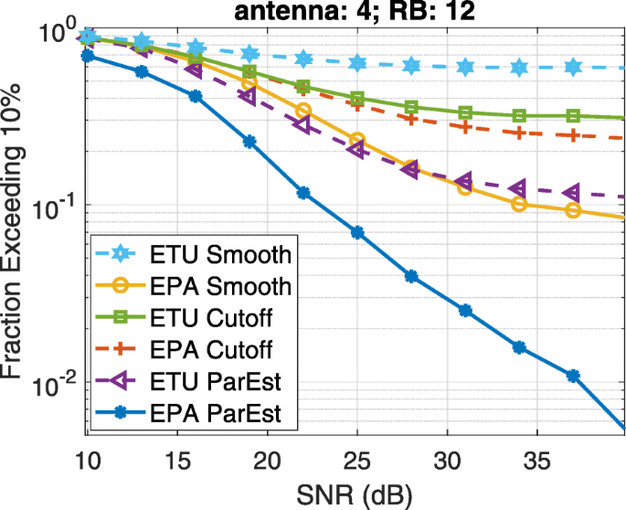

  

  Fractions of error over 10%. 4 antennas

  Fig. 9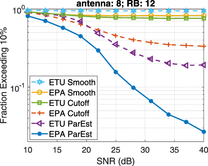

  

  Fractions of error over 10%. 8 antennas

  Fig. 10

  

  Bit error ratio. 4 antennas

  Fig. 11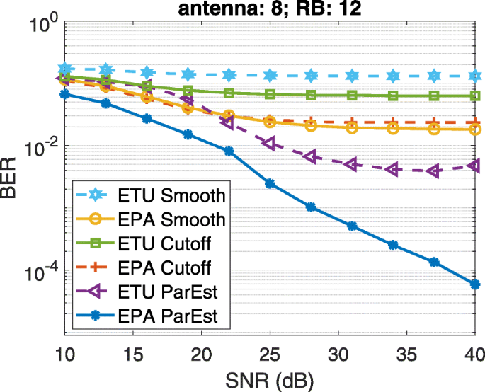

  

  Bit error ratio. 8 antennas

• The gain of ParEst for ETU channel is smaller than the EPA channel, because ETU has larger delay spread and is more difficult to approximate.

• The performance of ParEst consistently improves as SNR increases. On the contrary, the performance of Cutoff and Smooth seems to be stagnant even with higher SNR, especially for 8 antennas. This is because of the systematic errors of these methods cannot be reduced with higher SNR. Note that Cutoff approximates the entire peak vector with only points around the peak, while Smooth assumes that neighboring subcarriers have the same channel.

7.2.5 Computation complexity of ParEst

Figure 12 shows the run-time computation complexity of ParEst as a function of SNR, measured by the number of iterations in the linear search. Note that the upper bound of the complexity is linear to the number of iterations according to the analysis in Section 4.4. The observations are in the following:

• The computation complexity of ParEst is indeed very low. For example, even for the more challenging case under the ETU channel, the number of iterations, at most, is just slightly below 35. Such a number of iterations should put no burden on the implementation in practice, considering that the computation in each iteration is very simple.

  Fig. 12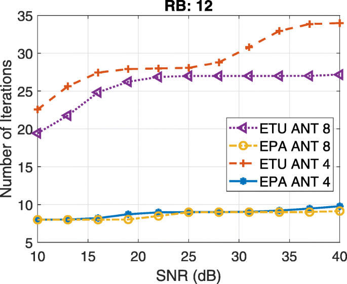

  

  Computation complexity of ParEst

• The computation complexity is lower for simpler channels. This is because simpler channels have smaller delay spread and need less sinusoids to approximate. It also shows that ParEst is able to automatically select parameters to match the channel condition.

• The number of iteration increases as the SNR increases. This is because as the SNR increases, more fine details in the CSI curves are revealed, which require more base sinusoids to match.

8 Conclusions

In this paper, a novel CSI estimation method, ParEst, is proposed. ParEst is designed for senders with multiple antennas and allows the sender to transmit CSI training symbols simultaneously on all antennas. The receiver solves an optimization problem based on the received composite signal and finds the CSI of each individual antenna. The run-time complexity of ParEst is very low, because most of the steps are pre-computed, based on the fact that the CSI can be approximated very well by sinusoids on constant frequencies. ParEst has been experimentally tested and has been shown to be capable of estimating the CSI in the real-world. ParEst has also been compared with the existing methods with simulations and has demonstrated improvements of over an order of magnitude in many cases. Therefore, ParEst can be a strong candidate as the CSI estimation method for networks such as LTE, 5G, and Wi-Fi.

References

A. Mukherjee, Z. Zhang, Fast compression of OFDM channel state information with constant frequency sinusoidal approximation. EURASIP J. Wirel. Commun. Netw.2019:, 87 (2019). https://doi.org/10.1186/s13638-019-1409-1.
A. Ancora, C. Bona, D. T. M. Slock, in 2007 IEEE International Conference on Acoustics, Speech and Signal Processing-ICASSP’07. Down-sampled impulse response least-squares channel estimation for LTE OFDMA, (2007), pp. 293–296.
M. Morelli, U. Mengali, A comparison of pilot-aided channel estimation methods for OFDM systems. IEEE Trans. Signal Process.49(12), 3065–3073 (2001).
G. Y. Li, Simplified channel estimation for OFDM systems with multiple transmit antennas. IEEE Trans. Wirel. Commun.1(1), 67–75 (2002).
S. Sesia, I. Toufik, M. Baker, LTE-the UMTS long term evolution: from theory to practice, 2nd Edition (John Wiley & Sons Ltd., 2011).
3GPP TS 38.211. NR; Physical channels and modulation (Release 15). 3rd Generation Partnership Project; Technical Specification Group Radio Access Network.
X. Hou, Z. Zhang, H. Kayama, in Proceedings of the 70th IEEE Vehicular Technology Conference Fall. DMRS design and channel estimation for LTE-advanced MIMO uplink, (2009), pp. 1–5. https://doi.org/10.1109/VETECF.2009.5378829.
Y. Xie, Z. Li, M. Li, in International Conference on Wireless Communications & Signal Processing. Efficient channel estimation for LTE uplink, (2009), pp. 1–5.
M. Jiang, G. Yue, N. Prasad, S. Rangarajan, in Proceedings of the 75th IEEE Vehicular Technology Conference (VTC Spring). Enhanced DFT-based channel estimation for LTE uplink, (2012), pp. 1–5. https://doi.org/10.1109/VETECS.2012.6240325.
S. Pratschner, E. Zöchmann, M. Rupp, Low complexity estimation of frequency selective channels for the LTE-A uplink. IEEE Wirel. Commun. Lett.4(6), 673–676 (2015).
S. Pratschner, S. Schwarz, M. Rupp, in IEEE International Conference on Communications (ICC). Single-user and multi-user MIMO channel estimation for LTE-Advanced uplink, (2017), pp. 1–6.
H. Tran, T. Mai, D. Vuong, N. Nguyen, in IEEE 5G World Forum (5GWF). On improvement of channel estimation for the uplink of large scale MU-MIMO using DMRS, (2018), pp. 294–298.
Z. Gao, L. Dai, Z. Lu, C. Yuen, Z. Wang, Super-resolution sparse MIMO-OFDM channel estimation based on spatial and temporal correlations. IEEE Commun. Lett.18(7), 1266–1269 (2014).
Y. Barbotin, M. Vetterli, Estimation of sparse MIMO channels with common support. IEEE Trans. Commun.60(12), 3705–3716 (2012).
J. Choi, D. Love, P. Bidigare, Downlink training techniques for FDD massive MIMO systems: open-loop and closed-loop training with memory. IEEE J. Sel. Top. Signal Process.8(5), 802–814 (2014).
W. Bajwa, J. Haupt, A. Sayeed, R. Nowak, Compressed channel sensing: a new approach to estimating sparse multipath channelsy. Proc. IEEE. 98(6), 1058–1076 (2010).
X. Rao, V. Lau, Distributed compressive CSIT estimation and feedback for FDD multi-user massive MIMO systems. IEEE Trans. Signal Process.62(12), 3261–3271 (2014).
J. -C. Shen, J. Zhang, E. Alsusa, K. B. Letaief, in IEEE International Conference on Communications (ICC). Compressed CSI acquisition in FDD massive MIMO with partial support information, (2015), pp. 1459–1464.
M. Biguesh, A. Gershman, Training-based MIMO channel estimation: a study of estimator tradeoffs and optimal training signals. IEEE Trans. Signal Process.54(3), 884–893 (2006).
Y. Liao, X. Yang, H. Yao, L. Chen, S. Wan, Spatial correlation based channel compression feedback algorithm for massive MIMO systems. Digit. Signal Process.94:, 38–44 (2019).
H. Cho, T. Nguyen, H. N. Nguyen, H. Choi, J. Choi, S. Ro, V. D. Nguyen, A robust ICI suppression based on an adaptive equalizer for very fast time-varying channels in LTE-R systems. EURASIP J. Wirel. Commun. Netw.2018:, 17 (2018).
T. Nguyen, T. H. Nguyen, T. Yoon, W. Jung, D. Yoo, S. Ro, An ICI suppression analysis testbed for harbor unmanned ground vehicle deployment. IEEE Access. 7:, 107757–107768 (2019).
J. -K. Choi, V. D. Nguyen, H. N. Nguyen, V. V. Duong, T. H. Nguyen, H. Cho, H. -K. Choi, S. -G. Park, A time-domain estimation method of rapidly time-varying channels for OFDM-based LTE-R systems. Digit. Commun. Netw.5:, 94–101 (2019).
D. Vasisht, S. Kumar, H. Rahul, D. Katabi, in Proceedings of the 2016 ACM SIGCOMM Conference. Eliminating channel feedback in next-generation cellular networks, (2016), pp. 398–411.
H. Xie, F. Gao, S. Jin, J. Fang, Y. Liang, Channel estimation for TDD/FDD massive MIMO systems with channel covariance computing. IEEE Trans. Wirel. Commun.17(6), 4206–4218 (2018). https://doi.org/10.1109/TWC.2018.2821667.
M. B. Khalilsarai, S. Haghighatshoar, X. Yi, G. Caire, FDD massive MIMO via UL/DL channel covariance extrapolation and active channel sparsification. IEEE Trans. Wirel. Commun.18(1), 121–135 (2019). https://doi.org/10.1109/TWC.2018.2877684.
J. Zhao, H. Xie, F. Gao, W. Jia, S. Jin, H. Lin, Time varying channel tracking with spatial and temporal BEM for massive MIMO systems. IEEE Trans. Wirel. Commun.17(8), 5653–5666 (2018). https://doi.org/10.1109/TWC.2018.2848259.
Y. Han, T. Hsu, C. Wen, K. Wong, S. Jin, Efficient downlink channel reconstruction for FDD multi-antenna systems. IEEE Trans. Wirel. Commun.18(6), 3161–3176 (2019). https://doi.org/10.1109/TWC.2019.2911497.
X. Wang, S. B. Wicker, in IEEE Global Communications Conference (GLOBECOM). Channel estimation and feedback with continuous time domain parameters, (2013), pp. 4306–4312.
A. Mukherjee, Z. Zhang, in 13th Annual IEEE International Conference on Sensing, Communication, and Networking (SECON). Channel state information compression for MIMO systems based on curve fitting, (2016), pp. 1–9.
A. Mukherjee, Z. Zhang, in IEEE (GLOBECOM). Fast compression of OFDM channel state information with constant frequency sinusoidal approximation, (2017), pp. 1–7.
Z. Zhang, A. Mukherjee, System and method for fast compression of OFDM channel state information (CSI) based on constant frequency sinusoidal approximation (2017). US Patent 9838104.
Z. Zhang, A. Mukherjee, in 2018 International Symposium on Networks, Computers and Communications (ISNCC). Joint channel estimation of multiple transmitters on shared resource blocks by approximating channel states with constant frequency sinusoids, (2018), pp. 1–4. https://doi.org/10.1109/ISNCC.2018.8531040.
3GPP TS 36.101. User equipment (UE) radio transmission and reception. 3rd Generation Partnership Project; Technical Specification Group Radio Access Network. Evolved Universal Terrestrial Radio Access (E-UTRA).
3GPP TS 36.104. Base station (BS) radio transmission and reception. 3rd Generation Partnership Project; Technical Specification Group Radio Access Network. Evolved Universal Terrestrial Radio Access (E-UTRA).
Ettus Research. https://www.ettus.com/all-products/ub210-kit/.
GNU Radio. http://gnuradio.org/.
OpenLTE – An open source 3GPP LTE implementation. https://sourceforge.net/projects/openlte/.
Funding
This research work was supported by the US National Science Foundation under Grant 1618358.
Author information
Authors and Affiliations
Contributions
Zhenghao Zhang is the sole contributor of this paper. The author(s) read and approved the final manuscript.
Corresponding author
Ethics declarations
Competing interests
The authors declare that they have no competing interests.
Additional information
Publisher’s Note
Springer Nature remains neutral with regard to jurisdictional claims in published maps and institutional affiliations.
Rights and permissions
Open Access This article is licensed under a Creative Commons Attribution 4.0 International License, which permits use, sharing, adaptation, distribution and reproduction in any medium or format, as long as you give appropriate credit to the original author(s) and the source, provide a link to the Creative Commons licence, and indicate if changes were made. The images or other third party material in this article are included in the article’s Creative Commons licence, unless indicated otherwise in a credit line to the material. If material is not included in the article’s Creative Commons licence and your intended use is not permitted by statutory regulation or exceeds the permitted use, you will need to obtain permission directly from the copyright holder. To view a copy of this licence, visit http://creativecommons.org/licenses/by/4.0/.
About this article
Cite this article
Zhang, Z. ParEst: joint estimation of the OFDM channel state information in MIMO systems. J Wireless Com Network 2020, 235 (2020). https://doi.org/10.1186/s13638-020-01833-y
Received:
Accepted:
Published:
DOI: https://doi.org/10.1186/s13638-020-01833-y