An adaptive transmission protocol for exploiting diversity and multiplexing gains in wireless relaying networks

Abstract

Wireless relaying networks with distributed space-time block codes have been shown to provide high link reliability. This is because of the space diversity gain from multiple transmitting relays, which improves by adding more relays. The drawback of this approach is the overall reduction in throughput of the network. In this paper, we propose a method to construct a distributed space-time block code that is combined with spatial modulation to find a flexible trade-off between reliability and throughput. This proposed method is not restricted to a specific number of relays and can be constructed as necessary. The constructed code also uses a novel adaptive transmission protocol to achieve higher space diversity, even with relays equipped with a single antenna. This protocol assumes use of coherent detection, meaning that a perfect channel estimation is available at the destination. Lastly, a new decoder is proposed that offers significant reduction in complexity to maintain high data throughput. All claims in this work are supported with theoretical analysis and backed up with empirical results.

1 Introduction

In recent years, the spatial diversity of wireless relaying networks (WRNs) has been used to improve signal quality in wireless transmission [1-5]. A WRN constructs a virtual multiple-input multiple-output (MIMO) system using multiple neighbouring client apparatuses as relaying nodes. It has been suggested that distributed space-time block codes (D-STBC) be used in WRNs to allow simultaneous transmission among relaying nodes to increase the spectral efficiency of the network [6-9]. It is known that the diversity is further improved when the number of relays in the WRN is increased. Unfortunately, this has the drawback of reducing the overall throughput of the network as the number of relays increase [10]. The throughput can be retained by increasing the code rate of the D-STBC at the cost of decoding complexity [11]. It has been shown that an orthogonal design of full-rate codes is possible only with two relays [12]. The orthogonal designs lead to a low decoding complexity at the destination[11].

To summarise, the major challenge in WRNs is to coordinate an arbitrary number of relay transmissions with high rate while maintaining both full diversity and low decoding complexity.

1.1 Prior work

The overall interest in this field of research lies in the construction of a high-rate D-STBC that has the ability to utilise any arbitrary number of relays [13,14]. It would appear that research has had limited success in designing high-rate codes while maintaining a single-symbol decodability at the destination. In [15], the authors proposed systematic construction steps of a row-monomial D-STBC with a code rate bounded by 2/(2+N), where N denotes the number of relays. In [16], a new code class called semi-orthogonal precoded distributed single-symbol decodable STBC (Semi-PD-SSD-STBCs) was proposed. It has the advantage of performing precoding on the information symbols, which in turn doubles the achieved code rate. Although these codes were designed for an arbitrary number of relays, they may be preferable to be used only in WRNs with a few number of relays. This is because the code rate decreases dramatically as the number of relays increases. In [17], a coding scheme, with a code rate of $\frac {1}{4}$, was proposed to operate in WRNs of high number of relays. However, this scheme has a high decoding delay. This is as the required transmission time increases exponentially with the number of relays. In [18], an adjustable full-rate STBC matrix was designed, but it requires a feedback channel to adjust the code. This creates additional network overhead that inherently reduces the achieved diversity gain. In [19-21], the generalised ABBA code (GABBA) of [22] was adapted for amplify-and-forward (AF) WRNs to offer a full-rate while maintaining single-symbol decodability. However, the resulting D-GABBA scheme has some constraints: (1) the number of symbols per block (T) should be expressible as a power of two, and (2) the number of available relays (N) should be smaller or equal to T (N≤T). These constraints were resolved by utilising global knowledge of channel state information (CSI) of the entire WRN at the relays [10].

Spatial modulation (SM) was developed to improve the throughput of MIMO systems and was initially extended for WRNs in [23-25]. The intention was to add the spatial dimension to the modulated signal constellation; this allowed information to be transmitted not only using amplitude/phase modulation (APM) but also using the relay index. This offers higher throughput due to data multiplexing via different relays [24,26]. However, the overall achieved diversity gain was limited to the number of receive antennas, as only one relay was active for any given transmission. This was partially solved when employing SM specifically at the source node and leaving the full diversity gain to be achieved in the link between the relays and the destination [25,27,28]. The effective use of SM was still bounded by the number of antennas available at the source node. Due to size, cost and hardware limitations, the availability of multiple antenna may not be feasible in many systems [29]. In [30,31], transmit diversity gain can be achieved at the expense of orthogonal channel resources.

In conclusion, the current WRN uses its relays either to offer high throughput only (using SM) or to achieve transmit diversity gain (using D-STBC).

1.2 Our contribution

As mentioned, a major challenge in a WRN is to coordinate an arbitrary number of relay transmissions while maintaining full diversity gain and offering high rates with low decoding complexity at the destination. Using a combination of STBC and SM, it is expected that high throughput and high transmit diversity gain is possible. In general, such combinations are achieved using MIMO systems. This allows the construction of a fixed STBC-SM code as the number of antennas at the transmitter is fixed [32-36]. These designs are also bounded by a transmit diversity gain of 2. To the best of the authors’ knowledge, there is no existing research addressing distributed STBC-SM (D-STBC-SM). With respect to the current literature, this paper presents:

• An adaptive transmission protocol to accommodate N relays in decode-and-forward (DF) WRNs, where $N \in \mathbb {N}^{+}$. Unlike [32-36], this protocol offers a transmit diversity gain of N ₀ (N≤N ₀≤1) because the possibility of activating N ₀ number of relays simultaneously during transmission. Given some control information, the protocol can be adapted to transmit through any given number of relays (N ₀). This means the network can work with a varying number of N ₀, which is a desirable feature for networks that experience imperfect time synchronisation [37,38].

• An algorithm to construct D-STBC-SM codes. Unlike [15,16,19-21], this algorithm offers a rate that increases with the number of relays. The rate for this code is $r_{0} \text {log}_{2} M_{2}+\frac {1}{T_{2}}\text {log}_{2} c$ bpcu instead of r ₀log₂ M ₂ bpcu, where $c=\left \lfloor \left (\begin {array}{c} N\\N_{0}\end {array}\right)\right \rfloor _{2^{p}}$ is the number of possible relay combinations, r ₀ is the code rate of the used STBC, M ₂ is the order of modulation used by the relays and ⌊.⌋ represents the floor integer operator. The increase in throughput uses the same total average transmitting energy. This is as only N ₀ of the N available participating relays are active at any given time. The proposed algorithm uses multi-level optimisation processes, and hence the constructed code outperforms the few existing STBC-SM codes.

• An optimal and suboptimal reduced-complexity decoder to work for the proposed protocol. The orthogonal property of the STBC allows a decoding complexity to reduce from $\mathcal { O}\left (cM_{2}^{n_{s}}\right)$ to $\mathcal { O}(cn_{s}M_{2})$, where n _s is the number of symbols per information block of transmission. Using the sub-optimal decoder, this decoding complexity can be further reduced to $\mathcal { O}(c+n_{s}M_{2})$ with some performance penalty. This makes it suitable to acquire higher throughput.

• Theoretical analysis of diversity gain, coding gain and required decoding complexity of the proposed protocol. Also, these claims are backed up by numerical simulations.

This paper is organised as follows: First, the network model is described followed by an outline of the proposed transmission protocol. Designing the D-STBC-SM code is then discussed. This is followed by a theoretical analysis of performance and complexity. Last, empirical results to back up the claims are presented.

1.3 Notations

Hereafter, small letters, bold small letters and bold capital letters will designate scalars, vectors and matrices, respectively. If A is a matrix, then A ^H, A ^∗ and A ^T denote the hermitian, conjugate and the transpose of A, respectively.

2 Network model

A dual-hop WRN comprised a source , $\hat {N}$ number of half-duplex (HD) relays $R_{1},\ldots,R_{\hat {N}}$ and a destination is considered (depicted in Figure 1). Let the source and relays be equipped with a single antenna and the destination has N _r antennas, $N_{r}\in \mathbb {N}^{+}$. This configuration is denoted by $\left (\hat {N},N_{r}\right)$. The transmission through the network is conducted in two phases. In the first phase, the information is broadcast from the source to the relays. In the second phase, each relay decodes its received symbols which are then only encoded and transmitted to the destination if received correctly. The total transmission power for the entire network is denoted by P and is evenly divided between both phases. The channel through the network is assumed to be a quasi-static Rayleigh fading channel. The source is assumed to be completely blind, while perfect CSI is assumed only at the decoding nodes.

Figure 1

Wireless relaying network model. A graph model of a WRN, given that N out of $\hat {N}$ relays are active in the relaying phase. It is assumed that both source and each relay are equipped with a single antenna while the destination has N _r antennas.

3 The proposed transmission protocol

In this section, an adaptive protocol that uses an efficient combination of D-STBC and SM is proposed to obtain better cooperative diversity gain and higher overall throughput. This will be supported by a mathematical evaluation and an empirical comparison to existing protocols on bit error rate (BER) graphs.

3.1 Protocol description

For a network configuration of $\left (\hat {N},N_{r}\right)$, the transmission through the network is conducted in two phases:

Broadcasting phase:

The source transmits M ₁-ary PSK/QAM modulated symbols denoted by y(i)=[y(i,1),…,y(i,J)]^T, where i denotes the information block index and J is the number of symbols in the broadcasting phase. To maximise the number of participating relays, the source () uses an error control code (ECC) to mitigate all errors. This is as relays are only allowed to transmit if no error is present (see IEEE 802.16j standard of [39]). Thus, the received vector at R _n is

$$ \underset{J\times 1}{\mathbf{r}_{n}(i)}=g_{n}\underset{J\times 1}{\mathbf{y}(i)} +\underset{J\times 1}{\mathbf{v}_{n}(i)}, $$

((1))

where g _n ($g_{n} \sim \mathcal { C} \mathcal { N}(0,1)$) is the channel coefficient for the link between and R _n . The vector v _n is the noise at R _n with entries $v_{n} \sim \mathcal { C} \mathcal { N}\left (0,\sqrt {\frac {2}{P}}\right)$.

Multiplexing and relaying phase:

To match the proposed modifications, this phase’s name is changed to ‘multiplexing and relaying phase’ rather than ‘relaying phase’. As stated previously, a relay will not partake in this phase if it detects an error. To limit the discussion, it is assumed that a fixed number N out of $\hat {N}$ relays will always have no errors. The participating N relays will each conduct the following on its K=Jlog₂ M ₁ received bits (illustrated in Figure 2):

• 1. The K decoded bits are divided into two groups. The first group contains K ₁ bits, and it is multiplexed to determine the relays that will be used to transmit the second group of K ₂ bits. These K ₂ bits are modulated and then encoded with the D-STBC. If K≠K ₁+K ₂, the excess bits must be buffered. The values of K ₁ and K ₂ are chosen according to Section 2.

  Figure 2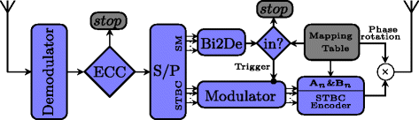

  

  Multiplexing and relaying phase for a given relay node. An illustration of the steps that each relay is conducting for each block of transmission.

• 2. The binary sequence of the first group is converted to a decimal value ℓ. This value is used to determine if the relay is allowed to transmit and what it should transmit. The second group of K ₂ bits is modulated to a symbol vector y ₂(i)=[y ₂(1,i),…,y ₂(n _s ,i)]^T using a two-tier star M ₂-ary QAM modulator (see Section 2).

• 3. Given ℓ, the relay R _n encodes its second group of K ₂ bits with a column of the D-STBC. The column index is obtained from the entries given in the code-mapping table. This encoding process is expressed as

  $$ \underset{L \times 1}{\mathbf{t}_{n}(i)}=\underset{L \times n_{s}}{\mathbf{A}_{n_{\ell}}}\underset{n_{s}\times 1}{\mathbf{y}_{2}(i)}+\underset{L \times n_{s}}{\mathbf{B}_{n_{\ell}}}\underset{n_{s} \times 1}{\mathbf{y}_{2}^{*}(i)}, $$

  ((2))

  where L=n _s /r ₀ and r ₀ is the code rate of the code used. n _ℓ is the logic index used to identify the encoding matrices that should be used at relay R _n . Both $\mathbf {A}_{n_{\ell }}$ and $\mathbf {B}_{n_{\ell }}$ are the encoding matrices responsible for generating the column n _ℓ of the D-STBC matrix. All of $\mathbf {A}_{n_{\ell }}$ and $\mathbf {B}_{n_{\ell }} \left (n_{\ell }=1\ldots N_{0}\right)$ are characterized by the D-STBC matrix and are used to construct the code in a distributive manner (see Appendix Appendix 1: Example STBC encoding matrices) [11,29]. It is worth noting that many existing D-STBC matrix can be used, given the number of relays and the extent of the diversity gain required (N ₀). This will be discussed in detail in Section 2.

• 4. The vector t _n (i) is then phase-rotated to ensure maximum diversity and coding gain. If the rotation is not used, then rank deficiency occurs due to interfering codewords and the achieved diversity gain is reduced. This results in the transmitted vector given as $\mathbf {t}^{\theta }_{n}(i)=\text {exp}(j\theta _{i})\mathbf {t}_{n}(i)$, where θ _i , θ _i ∈[0,π] are provided by the code-mapping table.

Accordingly, the received symbol matrix at destination is given by

$$ \underset{L\times N_{r}}{\mathbf{Z}(i)}=\sum_{n=1}^{N_{0}}\underset{L\times 1}{\mathbf{t}^{\theta}_{n}(i)}\underset{1\times N_{r}}{\mathbf{h}_{n}} +\underset{L\times N_{r}}{\boldsymbol{\eta}(i)}, $$

((3))

where $\mathbf {h}_{n}=\left [h_{n,1},\ldots,h_{n,N_{r}}\right ]^{T}$ is the channel coefficient vector from the relay R _n to the destination with entries $h_{n,j} \sim \mathcal { C} \mathcal { N}(0,1)$. The matrix η is the noise at the destination with entries $\eta _{\textit {ij}} \sim \mathcal { C} \mathcal { N}\left (0,\sqrt {\frac {2}{P}}\right)$.

The received signal matrix of (3) can be rewritten using (2) as

$$ \mathbf{z}(i)=\boldsymbol{\mathcal{ H}}_{\ell}\mathbf{y}_{2}(i)+\boldsymbol{\eta}(i), $$

((4))

where $\boldsymbol {\mathcal { H}}_{\ell }$ is the equivalent channel matrix that encapsulates both the rotation employed and the channel coefficients of the relay set ℓ used for transmission.

3.2 D-STBC-SM system design and optimisation

3.2.1 Review of conventional STBC-SM

Recently, the design of STBC-SM codes has drawn attention because of the promising improvements shown [32-36]. In this section, background and some required definitions of STBC-SM that are needed to work for D-STBC-SM are shown.

Definition 1.

The STBC scheme is represented by a matrix expressed as

$$ \underset{L \times N}{\mathcal{ X}}=\left [ \begin{array}{cccc} x_{1,1}&x_{1,2}&\cdots&x_{1,N}\\ x_{2,1}&x_{2,2}&\cdots&x_{2,N}\\ \vdots&\vdots&\cdots&\vdots\\ x_{L,2}&x_{L,2}&\cdots&x_{L,N}\\ \end{array} \right ], $$

((5))

where the columns represent the encoded L time-slot sequences that should be transmitted by the N transmitting antennas of the source. If n _s denotes the number of encoded symbols, then the code rate r of the used STBC is defined as $r=\frac {n_{s}}{L}$. ■

Definition 2.

Let X denote the STBC matrix (see Definition 1) and the STBC-SM code word denoted by X _i,j [32]. An STBC-SM codebook $\mathcal { X}_{d}$ is defined as a set of n _X STBC-SM codewords. The STBC-SM code is, here, formally defined as a set of $n_{\mathcal { X}}$ codebooks. ■

Definition 3.

Let be an STBC-SM code with $n_{\mathcal { X}}$ codebooks, and each has n _X codewords. The minimum coding gain distance (CGD) is defined by

$$ \alpha(\mathcal{ X})=\min_{i,j}\gamma_{\min}(\mathcal{ X}_{i}, \mathcal{ X}_{j}), $$

((6))

where $i,j=1\ldots n_{\mathcal { X}}$ and $\gamma _{\min }(\mathcal { X}_{i}, \mathcal { X}_{j})$ is the minimum CGD between two codebooks given by

$$ \gamma_{\min}(\mathcal{ X}_{i}, \mathcal{ X}_{j})= \underset{k,l}{\min} \mathbf{H}_{\lambda}(\mathbf{X}_{ik}, \hat{\mathbf{X}}_{jl}|i\neq j \& k \neq l). $$

((7))

The variables l,k=1…n _X , $\mathbf {H}_{\lambda }\left (\mathbf {X}_{\textit {ik}}, \hat {\mathbf {X}}_{\textit {jl}}\right)$ are the harmonic mean of the non-zero eigenvalues of $\mathbf {A}\left (\mathbf {X}_{\textit {ik}}, \hat {\mathbf {X}}_{\textit {jl}}\right)= \Delta \left (\mathbf {X}_{\textit {ik}}, \hat {\mathbf {X}}_{\textit {jl}}\right)\Delta ^{H}\left (\mathbf {X}_{\textit {ik}}, \hat {\mathbf {X}}_{\textit {jl}}\right)$, and $\Delta \left (\mathbf {X}, \hat {\mathbf {X}}\right)=\mathbf {X}-\hat {\mathbf {X}}$. ■

The STBC-SM code exploits the properties of SM by distributing the STBC codeword over a subset of the number of antennas at the transmitter. The number of antennas at the transmitter is fixed. This allows the construction only of a fixed STBC-SM code. For example, codewords of an STBC-SM code () proposed in [32] is based on Alamouti’s STBC for a 4×1 MIMO system which are expressed as

$$ {\fontsize{8}{6}\begin{aligned} {\mathcal{X}}_{1}=\left \{\mathbf{X}_{11},\mathbf{X}_{12} \right \} =\left \{ \left (\begin{array}{cccc} \mathbf{y}(1)&\mathbf{y}(2)&0&0\\ -\mathbf{y}^{*}(2)&\mathbf{y}^{*}(1)&0&0\\ \end{array} \right),\left (\begin{array}{cccc} 0 & 0 & \mathbf{y}(1)&\mathbf{y}(2)\\ 0 & 0 & -\mathbf{y}^{*}(2)&\mathbf{y}^{*}(1)\\ \end{array} \right)\right \} \end{aligned}} $$

((8))

$$ {\fontsize{7.5}{6}\begin{aligned} \mathcal{ X}_{2}=\left \{\mathbf{X}_{21},\mathbf{X}_{22} \right \} =\left \{ \left (\begin{array}{cccc} 0&\mathbf{y}(1)&\mathbf{y}(2)&0\\ 0&-\mathbf{y}^{*}(2)&\mathbf{y}^{*}(1)&0\\ \end{array} \right),\left (\begin{array}{cccc} \mathbf{y}(2)&0&0&\mathbf{y}(1)\\ \mathbf{y}^{*}(1)&0&0&-\mathbf{y}^{*}(2)\\ \end{array} \right)\right \}e^{j\theta}. \end{aligned}} $$

((9))

In this STBC-SM design, the first 2 bits are used to decide on the codeword X _ij . These bits define the set of antennas to transmit the remaining encoded bits (y(1) and y(2)). It should be noted that each codeword X _ij uses a unique antenna mapping pattern. The phase rotation θ _i is set to avoid rank deficiency among codebooks to mitigate diversity gain loss. The designs of a more complex STBC-SM in a MIMO system have shown promising improvements and recently have started to attract attention [32-36].

3.2.2 D-STBC-SM code construction

In a conventional MIMO system, the number of antennas at both the destination and source is fixed. In contrast, the number of transmitting antennas is determined by the number of available relays in WRNs. The number of relays can differ for each initiated transmission, a variation that equates to the need for a D-STBC-SM code to operate over a varying distributed network. In this section, an algorithm is defined to construct D-STBC-SM codes to work in WRNs. Two examples of constructing a D-STBC-SM code for given WRNs are also provided.

The construction of an optimal D-STBC-SM code relies on the proper selection of a relay index pattern that maximises the CGD. To reduce the search space for the optimised codebooks, the inner and mutual CGDs are formally defined:

Definition 4.

For a given , the inner CGD ($\varphi _{\min }(\mathcal { X})$) and the mutual CGD ($\delta _{\min }(\mathcal { X})$) are given by

$$ \varphi_{\min}(\mathcal{ X})=\min_{i}\gamma_{\min}(\mathcal{ X}_{i}, \mathcal{ X}_{i}) $$

((10))

and

$$ \delta_{\min}(\mathcal{ X})=\min_{i,j}\gamma_{\min}(\mathcal{ X}_{i}, \mathcal{ X}_{j}) \forall\ i \neq j, $$

((11))

respectively. ■

Another two important metrics in the construction of the code are how the relay patterns are chosen, namely the indexing distance and the Hamming distance. Both are used in the shown algorithm and are formally defined as

Definition 5.

Let {R _i } and {R _j }, $i \text {and }j \in \mathbb {N}$, denote two sets of relays. Then, $\rho : \mathbb {N} \rightarrow |(\{R_{i}\}\cap \{R_{j}\})|$ defines the indexing distance. This computes the size of the intersection between these two sets. ■

Definition 6.

Let {R _i } and {R _j }, $i \text {and }j \in \mathbb {N}$, denote two sets of relays with similar cardinality. Then, $d_{\text {min}}: \mathbb {N} \rightarrow (\{R_{i}\},\{R_{j}\})$ defines the Hamming distance between the two sets of relays. ■

To maximise the BER performance, the proposed algorithm is designed to construct codewords with minimal indexing distance ρ and maximum Hamming distance d _min. This design can operate on the common modulation schemes, but an additional improvement was observed using star QAM. The star QAM relies on two parameters that are also optimised in the algorithm as an additional step and, for completeness, are defined in Definition 7.

Definition 7.

A two-tier star M-ary QAM modulation has its constellation points distributed over two amplitude levels a and b. There are $\frac {M}{2}$ constellation points on each amplitude level with a phase difference ϕ [40], as depicted in Figure 3.

Figure 3

Two-tier star M -ary QAM constellation. A graph illustration of the two-tier star 8-ary QAM constellation.

Both a and ϕ should be optimised to maximise codeword differences. $b=\sqrt {2-a^{2}}$ should hold to ensure a unity average transmitted power. ■

Now with the necessary definitions, the proposed algorithm can be described in detail in Algorithm 1. Two examples are provided to illustrate how the algorithm operates. The codes shown below follow step by step in its construction phase. The algorithm shown have a code rate of

$$ r=r_{0}\text{log}_{2}M_{2}+\text{log}_{2}c, $$

((12))

where r and r ₀ are the code rate of the constructed D-STBC-SM and the STBC used, respectively.

The overall rate increases as the number of relays increases. This is seen in (12) for a number of participating relays (examples are shown in Table 1).

Table 1 The code rate for a different number of relays

Example 1.

Let N ₀=2 and N=4, then the number of possible combinations is c=4. A D-STBC-SM is constructed based on the proposed algorithm while using Alamouti’s STBC shown in Appendix Appendix 1: Example STBC encoding matrices. For illustration purposes, the optimisation process results are shown in Appendix Appendix 2: Optimising a code-mapping table. The STBC-SM proposed in [32] that was originally designed for a conventional MIMO system can be used on this WRN, but Section 2 shows an improvement when using the proposed algorithm. The final constructed code-mapping table is given in Table 2. ■

Table 2 The code-mapping table for Example 1

Example 2.

Let N ₀=3 and N=6, then the number of possible combinations is c=8. A D-STBC-SM is constructed using the STBC (with code rate $\frac {3}{4}$) of Appendix Appendix 1: Example STBC encoding matrices. The constructed code-mapping table is given in Table 3. To avoid repetition, the illustration of optimization process for this code is omitted. ■

Table 3 The code-mapping table for Example 2

3.3 Decoding methods

The growing demand for more complex WRN transmissions requires more complex decoders at the receiving node. In this section, an optimal maximum likelihood (ML) decoder for the transmission protocol is described, followed by a proposal of a reduced-complexity decoder.

3.3.1 Optimal ML decoder

The ML decoder considers an exhaustive search trying to estimate the transmitted data. This is expressed as

$$ \left[ \hat{\ell},\hat{\mathbf{y}_{2}} \right]=\operatornamewithlimits{arg min}_{\ell \in \left\{ 0,\ldots c-1 \right\}, \mathbf{y}_{2} \in \mathcal{ S}_{2}^{n_{s}} }||\mathbf{z}-\boldsymbol{\mathcal{ H}}_{\ell}\mathbf{y}_{2}||^{2}, $$

((14))

where $\mathcal { S}_{2}$ is the M ₂-ary star-QAM modulation used by the relays.

This equates to searching over all $cM_{2}^{n_{s}}$ permutations. Assuming an orthogonal STBC (OSTBC) is used, the received matrix can be decomposed into

$$ \hat{\mathbf{y}}_{2}^{\ell}(m) =\operatornamewithlimits{arg min}_{y_{2} \in \mathcal{ S}_{2}}||\mathbf{u}(m)-\beta y_{2}||^{2},\forall m={1,\ldots,n_{S}}, $$

((15))

and

$$ \hat{\ell}=\operatornamewithlimits{arg min}_{\ell}\left\{\sum_{m=1}^{n_{s}}\left(\min_{y_{2} \in \mathcal{ S}_{2}}||\mathbf{u}(m)-\beta y_{2}||^{2}\right)\right\}, $$

((16))

where $\mathbf {u}= \left [ \mathbf {u}(1), \mathbf {u}(2), \ldots, \mathbf {u}(n_{S})\right ]^{T}=\boldsymbol {\mathcal { H}}_{\ell }^{H}\mathbf {y}_{d}$ and $\boldsymbol {\mathcal { H}}_{\ell }^{H}\boldsymbol {\mathcal { H}}_{\ell }=\beta \mathbf {I}_{n_{s}}$.

This simplification based on the orthogonality property reduces the complexity of the decoder from $cM_{2}^{n_{s}}$ to n _s c M ₂.

3.3.2 Proposed reduced-complexity decoder

A further reduction in decoding complexity can be made using two sequential steps, with an accepted loss in BER performance. The first step determines the set of relays used in the relaying phase. This is accomplished by using a projection matrix P _ℓ with the condition that $\mathbf {P}_{\ell }\boldsymbol {\mathcal { H}}_{\ell }=0$. This projection matrix maps the received vector y _d to an orthogonal subspace $\boldsymbol {\mathcal { H}}_{\hat {\ell }}=\left [\begin {array}{cccc} \boldsymbol {\mathcal { H}}_{1}\ldots & \boldsymbol {\mathcal { H}}_{\ell -1} & \boldsymbol {\mathcal { H}}_{\ell +1} & \ldots \boldsymbol {\mathcal { H}}_{c}\end {array}\right ]$. The projection matrix is computed as

$$ \mathbf{P}_{\ell}=\mathbf{I}-\boldsymbol{\mathcal{ H}}_{\hat{\ell}}\left(\left(\boldsymbol{\mathcal{ H}}_{\hat{\ell}}\right)^{H}\boldsymbol{\mathcal{ H}}_{\hat{\ell}}\right)^{-1}\left(\boldsymbol{\mathcal{ H}}_{\hat{\ell}}\right)^{H}. $$

((17))

This matrix projects the received vector y _d to the space of $\boldsymbol {\mathcal { H}}_{\ell }$, which results in a product of zero for the correct set of relays if N _r ≥N ₀ and has no channel impairments. However, in the presence of channel impairments, the projection of the received vector z is altered and the decoder decides on the set of relays by

$$ \hat{\ell}=\operatornamewithlimits{arg min}_{\ell}||\mathbf{P}_{\ell}\mathbf{z}||^{2}. $$

((18))

It should be noted that there are numerous reduced-complexity (RC) detectors that appeared in the literature and that can be adapted for the first step of this sequential detector [44-46]. They differ in the offered performance complexity trade-off. The second step of this decoder is conducted using a traditional OSTBC decoder which computes [11]

$$ \hat{\mathbf{y}}_{2}(m)=\operatornamewithlimits{arg min}_{y \in \mathcal{ S}_{2}^{1 \times 1}}||\mathbf{u}(m)-\beta y||^{2}, $$

((19))

where $\mathbf {u}=\boldsymbol {\mathcal { H}}_{\hat {\ell }}^{H}\mathbf {z}$, and $\boldsymbol {\mathcal { H}}_{\hat {\ell }}^{H}\boldsymbol {\mathcal { H}}_{\ell }=\beta \mathbf {I}_{n_{s}}$ and $\mathbf {I}_{n_{s}}$ is n _s ×n _s identity matrix.

Thus, it can be observed that the number of all possible combinations for an ML search reduces from c n _s M ₂ to (c+n _s M ₂).

4 Performance analysis

In this section, the proposed transmission protocol is evaluated theoretically in terms of diversity gain, coding gain and the decoding complexity.

4.1 Diversity analysis

The diversity gain of a DF WRN is determined by the broadcasting or relaying phase that offers the lowest diversity gain individually. The scope of this work is focused on the diversity gain in the relaying phase. This section shows analysis of the diversity gain in the case of the optimal ML decoder and then in the case of the RC decoder.

4.1.1 ML decoder diversity analysis

Lemma 1.

If the diversity gain of an STBC code is N ₀×N _r , then constructing the D-STBC-SM based on Algorithm 1 using this STBC will also have a diversity gain of N ₀×N _r , if the ML decoder of Section 2 is used at the destination.

Proof.

It is known that a wireless communication system achieves a space diversity gain of d if the average error probability is upper bounded in the high SNR range by $\mathbb {P}\leq \alpha \gamma ^{-d}$, where $\alpha \in \mathbb {R}^{+}$ and it is independent of γ. γ is the SNR.

Assuming that a codeword X is transmitted through the relays, then (4) is equivalently written for a single-antenna destination as

$$ \mathbf{z}=\mathbf{X}\mathbf{h}+\boldsymbol{\eta}, $$

((20))

where h is the relays-destination channel vector.

Thus, the conditional pairwise error probability (PEP) of the WRN (see Section 2) can be computed as [47]

$$ \mathbb{P}(\mathbf{X} \rightarrow \hat{\mathbf{X}}|\mathbf{h})=Q\left(\sqrt{\frac{\gamma ||\Delta \mathbf{X} \mathbf{h}||^{2}}{2}}\right), $$

((21))

where $Q\left (x\right)=\int _{x}^{\infty }{e^{-y^{2}/2}\text {dy}}$. The error matrix is denoted by $\Delta \mathbf {X} =\mathbf {X}-\hat {\mathbf {X}}$.

Equation (21) can be expanded as

$$ \mathbb{P}(\mathbf{X} \rightarrow \hat{\mathbf{X}}|\mathbf{h})=Q\left(\sqrt{\frac{\gamma\left\Vert \tilde{\mathbf{h}}^{H}\Lambda\tilde{\mathbf{h}}\right\Vert^{2}}{2}}\right), $$

((22))

where $\Lambda =\text {diag}\left ({\lambda _{1}^{2}},\ldots,{\lambda _{N}^{2}}\right)$ and λ _n denotes the singular values of Δ X. V is a unitary matrix and $\tilde {\mathbf {h}}=\mathbf {V} \mathbf {h}$. It is worth noting that there is no rank deficiency in Λ due to using of the phase rotation (see Appendix Appendix 3: Rank of the constructed code).

Equation (22) can be simplified and bounded as

$$\begin{array}{@{}rcl@{}} \mathbb{P}(\mathbf{X} \rightarrow \hat{\mathbf{X}})&=&\mathbb{E}_{\mathbf{h}}\left(Q\left(\sqrt{\frac{\gamma\sum_{i=1}^{N_{0}}{\lambda_{i}^{2}}\left\Vert \tilde{\mathbf{h}}(i)\right\Vert^{2}}{2}}\right)\right)\\ &\leq & \mathbb{E}_{\mathbf{h}}\left(\text{exp}\left(\sqrt{\frac{\gamma\sum_{i=1}^{N_{0}}{\lambda_{i}^{2}}\left\Vert \tilde{\mathbf{h}}(i)\right\Vert^{2}}{4}}\right)\right). \end{array} $$

Given that the former code construction steps are followed, the rank of N ₀ is preserved (see Appendix Appendix 3: Rank of the constructed code). Thus, according to Lemma 1 of [48], the unconditional PEP is determined by

$$ \mathbb{P}(\mathbf{X} \rightarrow \hat{\mathbf{X}})\leq\prod_{n=1}^{N_{0}}\frac{1}{1+\gamma\frac{{\lambda_{n}^{2}}}{4}}, $$

((23))

which can be approximated for high SNR values as

$$ \mathbb{P}(\mathbf{X} \rightarrow \hat{\mathbf{X}})\lesssim\left(\frac{4}{\gamma}\right)^{N_{0}}\frac{1}{\prod_{n=1}^{N_{0}}{\lambda_{n}^{2}}}. $$

((24))

This concludes that a transmit diversity gain of N ₀ is achieved. As the equivalent channel matrix is a concatenation of the equivalent channel matrices of each receive antenna, it suffices to check the diversity gain for only one receiving antenna. This results in a diversity gain of N ₀×N _r for a code employed with an N _r -antenna destination.

4.1.2 Diversity analysis of RC decoder

It was shown that the designed D-STBC-SM code achieves the full diversity gain if the ML decoder is used. However, the RC decoder of Section 2 has limited diversity gain encapsulated in (18). It is limited by the relay combination detection step, which has an error probability $\mathbb {P}_{c}$ of

$$\begin{array}{@{}rcl@{}} \mathbb{P}_{c|\mathbf{H}} &=&1-\mathbb{P}(\nu_{\ell}\succ\nu_{\hat{\ell}_{1}},\ldots,\nu_{\ell}\succ\nu_{\hat{\ell}_{c-1}}|\ell,\mathbf{H})\\ &=&1-\mathbb{P}(\nu_{\ell}-\nu_{\hat{\ell}_{1}}=0|\ell,\mathbf{H})^{c-1} \\ &=&1-\left(\int_{0}^{\infty}f_{\nu_{\ell}-\nu_{\hat{\ell}_{1}}}(x)\text{dx}\right)^{c-1} \end{array} $$

((25))

$$\begin{array}{@{}rcl@{}} &=&\left(Q\left(\frac{\mu_{\ell}-\mu_{\hat{\ell}_{1}}}{\sqrt{\sigma_{\ell}^{2}+\sigma_{\hat{\ell}_{1}}^{2}}}\right)\right)^{c-1}. \end{array} $$

((26))

where with ${\sigma _{i}^{2}}={\sigma _{i}^{2}}\left \Vert \mathbf {P}_{\ell }\right \Vert ^{2}$, μ _i =P _ℓ H and

$$ f_{\nu_{\ell}-\nu_{\hat{\ell}_{1}}}(x)=\frac{1}{\sqrt{2\pi\left(\sigma_{\ell}^{2}+\sigma_{\hat{\ell}_{1}}^{2}\right)}}\exp\left(-\frac{\left(x-\mu_{\ell}-\mu_{\hat{\ell}_{1}}\right)^{2}}{2\left(\sigma_{\ell}^{2}+\sigma_{\hat{\ell}_{1}}^{2}\right)}\right) $$

This holds assuming that ν _ℓ =||P _ℓ z||² and information bits are independent and equiprobable.

By applying the Chernoff bound to (26), we can rewrite as

$$ \mathbb{P}_{c|\mathbf{F}}\leq\frac{1}{2^{c-1}}\exp\left(-\frac{c-1}{2}\frac{\left\Vert \boldsymbol{\mathcal{ H}}_{\ell}\right\Vert^{2}}{\sigma^{2}}\right). $$

((27))

Averaging over H, the relay combination detection error can be determined as

$$\begin{array}{@{}rcl@{}} \mathbb{P}_{c} &\leq&\int_{0}^{\infty}\frac{1}{2^{c-1}}\exp\left(-\frac{c-1}{2}\frac{x}{\sigma^{2}}\right)f_{||\boldsymbol{\mathcal{ H}}_{\ell}||^{2}}(x)\text{dx}\\ &=&\frac{1}{2^{c+N_{r}-1}\Gamma(N_{r})}\int_{0}^{\infty}\exp\left(-\frac{(c+\sigma^{2}-1)x}{2\sigma^{2}}\right)x^{N_{r}-1}\text{dx}\\ &\leq&\left(\frac{\sigma^{2}}{\sigma^{2}+c-1}\right)^{N_{r}} \\ &\leq&\left(\frac{1}{\left(c-1\right)\gamma}\right)^{N_{r}}. \end{array} $$

((28))

From (28), it can be concluded that the two-step decoder can achieve only the full-receive diversity gain N _r . Therefore, the complexity reduction is at the expense of transmit diversity gain.

4.2 Coding gain analysis

The coding gain of the proposed D-STBC-SM code is improved by maximising the CGD. The inner and mutual CGD of the code designed in Example 1 is compared with the code of [32] under the assumption of using an 8-ary modulation.

Thus, it can be observed that the proposed STBC-SM has a larger inner and mutual CGD than the code proposed in [32], and hence, better performance can be achieved (Table 4).

Table 4 CGD values of the proposed code and [ 32 ]

4.3 Complexity analysis

The complexity order is defined here as the number of iterations needed to find the optimal estimate for (4). The complexity order of the optimal ML decoder is $\mathcal {O}\left (cM_{2}^{n_{s}}\right)$, where n _s is the number of symbols per codeword and M ₂ is the order of the modulation used. This order is reduced to $\mathcal {O}(cM_{2}n_{s})$ when orthogonality of the STBC used is preserved. This is as orthogonality allows linear decomposition of the symbols. In contrast, the complexity order of the proposed RC decoder is further reduced to $\mathcal {O}(c+M_{2}n_{s})$. This is because the set of transmitting relays is firstly identified. A comparison of the complexity order is shown in Figure 4 in terms of the number of relays, for the configuration used in Example 1. The offered bits per channel use (bpcu) is also shown; this is determined by the number of relays and the modulation scheme. From Figure 4, it is observed that the complexity of the RC decoder increases marginally with the number of relays when compared to the complexity of the optimal ML decoder. The advantage of using the RC decoder is that the throughput can be increased from 3 to 4.5 bpcu for a 4-ary modulation scheme without complexity increasing at a cost of minor loss in performance.

Figure 4

Normalised complexity order versus the number of relays. Also, the offered bpcu is given in parentheses; the first value corresponds to an 8-ary case while the second value corresponds to a 16-ary case.

5 Simulation results

Numerical simulations are shown here in terms of BER to back up the theoretical claims of the proposed protocol. First, Example 1 and 2 networks are simulated and compared with a number of existing systems in Figures 5 and 6, respectively. This is to show how the proposed protocol and the constructed codes outperform the existing systems. Tables 5 and 6 summarise the simulation parameters used for the existing systems. This section shows also a comparison of using the optimal ML decoder and the RC decoder for different network configurations (shown in Figure 7). All simulations were conducted on a Rayleigh faded channel, and it was assumed that the total transmission power is evenly distributed between the transmission phases. For comparison purposes, the shown figures include two slope diversity gain reference curves for cases of (N×N _r ) and (N ₀×N _r ).

Figure 5

BER performance result of Example 1 network. The simulation results, in terms of BER, for the network configuration shown in Example 1.

Figure 6

BER performance result of Example 2 network. The simulation results, in terms of BER, for the network configuration shown in Example 2.

Figure 7

BER of (3,5,8)×4 D-STBC-SM when the optimal ML and RC decoder is used. The simulation results, in terms of BER, for the network configuration of (3,5,8)×4 D-STBC-SM. The results of using either the optimal ML decoder or the RC detector.

Table 5 Simulation parameters used in Figure 5

Table 6 Simulation parameters used in Figure 6

In Figure 5, the proposed transmission protocol (using the code in Example 1 on a (4²,4) network) is compared to Alamouti’s STBC, the $\frac {3}{4}$-OSTBC, the ABBA code and the traditional SM. Alamouti’s STBC is limited to only two relays and can achieve a transmit diversity gain of 2 (N ₀=2), while both the $\frac {3}{4}$-OSTBC and the ABBA code constantly utilise all four relays and achieve a transmit diversity gain of N ₀=N=4. However, they lose the throughput that can be offered by SM. The traditional SM offers better throughput at the cost of not using an STBC, which results in a loss of transmit diversity gain and coding gain. For a fair comparison in this experiment, no constraint was imposed on the modulation order used and the resulting system was required to provide a bpcu of 2. With reference to Figure 5, it is observed that the proposed protocol reports an improved BER performance. Specifically, it results in performance gains of 1.3, 2.3 and 3.6 dB over networks employing Alamouti’s STBC, $\frac {3}{4}$-OSTBC and ABBA code, respectively. In addition, a gain of 1 dB was achieved over the STBC-SM of [32] because of the unique selection of the c codewords and the use of optimised star-QAM modulation. It should be noted that this STBC-SM code of [32] was originally designed for a conventional MIMO system and was extended here to operate on the WRN for the purpose of this comparison.

The proposed protocol was simulated in Figure 6 for another network configuration of (6³,4) to investigate the ability to achieve higher diversity gain and to offer higher throughput. It was compared to an ABBA system which offers a transmit diversity gain of N ₀=N=6 by using all the available relays but without throughput improvement. A simulation of the traditional SM was included again to illustrate how the throughput can be maximised. It was observed that the proposed protocol had the lowest BER in this experiment with a diversity gain of (N ₀=3)×(N _r =4). It provides an SNR gain of 1.2 and 2.8 dB over networks employing the ABBA code and SM, respectively.

In the next experiment, the loss in performance in the case of using the RC decoder was investigated in Figure 7. It was compared to the optimal ML decoder in WRNs of (3²,4), (5²,4) and (8²,4). It should be noted that a reduction in complexity is ideal in certain applications when higher throughput is needed. In this experiment, it was observed that the optimal ML decoder achieved a diversity gain of (2×N _r =8), while the RC decoder had a reduced diversity gain of N _r =4.

6 Conclusions

Motivated by the developments in spatial modulation, an adaptive transmission protocol was proposed for WRNs to exploit the potential space diversity gain while obtaining higher spectral efficiency. Unlike the existing literature, this protocol can accommodate an arbitrary number of relays while improving the overall throughput and maintaining the same achieved space diversity gain. In addition, an algorithm to generate D-STBC-SM codes to be used by this protocol was shown. The achieved performance of the resulting codes is better than that of many existing codes because the criteria are designed to choose the codewords and to employ a multi-level optimization process. Also, a further reduced-complexity decoder is proposed. All of these claims are accompanied by numerical and theoretical evaluations.

7 Appendices

7.1 Appendix 1: Example STBC encoding matrices

For the sake of convenience the encoding matrix of each STBC used in the two examples are listed here. For Example 1, the full-rate Alamouti’s STBC code is used given as

$$ \mathcal{ X}=\left [ \begin{array} {cc} s(1,i)&s(2,i)\\ -s^{*}(2,i)&s(1,i)^{*}\\ \end{array} \right ], $$

((29))

with encoding matrices: A ₁=I ₂,B ₁=0 ₂,A ₂=0 ₂, and $\mathbf {B}_{2}=\left [ \begin {array} {cc} 0&-1\\ 1&0\\ \end {array} \right ]$.

In Example 2, a $\frac {3}{4}$-rate OSTBC code is used given as

$$ \mathcal{ X}=\left [ \begin{array} {ccc} s(1,i)&s(2,i)&s(3,i)\\ -s^{*}(2,i)&s(1,i)^{*}&0\\ -s^{*}(3,i)&0&s(1,i)^{*}\\ 0&s^{*}(3,i)&-s(2,i)^{*}\\ \end{array} \right ], $$

((30))

with encoding matrices:

$$\begin{array}{@{}rcl@{}} \mathbf{A}_{1}=\left [ \begin{array} {ccc} 1&0&0\\ 0&0&0\\ 0&0&0\\ 0&0&0\\ \end{array} \right ],\;\mathbf{A}_{2}=\left [ \begin{array} {ccc} 0&1&0\\ 0&0&0\\ 0&0&0\\ 0&0&0\\ \end{array} \right ], \end{array} $$

((31))

$$\begin{array}{@{}rcl@{}} \mathbf{A}_{3}=\left [ \begin{array} {ccc} 0&0&1\\ 0&0&0\\ 0&0&0\\ 0&0&0\\ \end{array} \right ],\; \mathbf{B}_{1}=\left [ \begin{array} {ccc} 0&0&0\\ 0&-1&0\\ 0&0&1\\ 0&0&0\\ \end{array} \right ], \end{array} $$

((32))

$$\begin{array}{@{}rcl@{}} \mathbf{B}_{2}=\left [ \begin{array} {ccc} 0&0&0\\ 1&0&0\\ 0&0&0\\ 0&0&1\\ \end{array} \right ], \;\text{and}\; \mathbf{B}_{3}=\left [ \begin{array} {ccc} 0&0&0\\ 0&0&0\\ -1&0&0\\ 0&-1&0\\ \end{array} \right ]. \end{array} $$

((33))

7.2 Appendix 2: Optimising a code-mapping table

The resulting figures of the optimization process of Example 1 code are shown here for illustration purposes. First, the parameters set {a,ϕ} for a M ₂-ary star-QAM modulation is chosen to maximise the inner CGD for the given code. In Figure 8, the inner CGD is shown over search ranges of a and ϕ. The values for the example was a=0.65 and ϕ=0.78 which provided a maximum inner CGD of 0.70.

Figure 8

The optimisation of a and ϕ value of the Example 1 network. An illustration of the optimisation process to determine the star-QAM parameters. It optimises the value of a and ϕ for the Example 1 network.

Another optimization which is crucial is to determine the correct phase rotation θ _i for each codebook. This is to avoid rank deficiency among codebooks to mitigate diversity gain loss. This is accomplished by choosing the set {θ _i } to maximise the mutual CGD. In Figure 9, the mutual CGD is shown for Example 1 for the search range of θ.

Figure 9

The optimisation of θ values for the Example 1 network. An illustration of the optimisation process for determining the optimal values of the phase-rotation among the codebooks. It optimises the value of θ for the Example 1 network.

7.3 Appendix 3: Rank of the constructed code

Following the steps of Algorithm 1, the constructed D-STBC-SM code based an STBC (), is with rank of N ₀, has the same rank of .

Proof.

Let {X} denote the set of codewords for a codebook $\mathcal { X}_{i}$. The rank of the constructed code in Example 1, computed from $\mathbf {A}(X,\hat {X})$ of (), is investigated to show that the maximum rate is preserved. There are two cases to consider: (1) when two codewords belong to the same codebook and (2) for the case of two different codebooks. In the first case, two codewords are present in the same codebook that used identical relays in its transmission. This results in

$$ \small{\mathbf{A}(\mathbf{X},\hat{\mathbf{X}})=\left [ \begin{array} {cccc} \sum_{n=1}^{N_{0}}{|x_{1n}-\hat{x}_{1n}|^{2}}&\sum_{n=1}^{N_{0}}{(x_{1n}-\hat{x}_{1n})(x_{2n}-\hat{x}_{2n})^{*}}&\ldots&\sum_{n=1}^{N_{0}}{(x_{1n}-\hat{x}_{1n})(x_{Ln}-\hat{x}_{Ln})^{*}}\\ \sum_{n=1}^{N_{0}}{(x_{2n}-\hat{x}_{2n})(x_{1n}-\hat{x}_{1n})^{*}}&\sum_{n=1}^{N_{0}}{|x_{2n}-\hat{x}_{2n}|^{2}}&\ldots&\sum_{n=1}^{N_{0}}{(x_{2n}-\hat{x}_{2n})(x_{Ln}-\hat{x}_{Ln})^{*}}\\ \vdots&\vdots&\ddots&\vdots\\ \sum_{n=1}^{N_{0}}{(x_{Ln}-\hat{x}_{Ln})(x_{1n}-\hat{x}_{1n})^{*}}&\sum_{n=1}^{N_{0}}{(x_{Ln}-\hat{x}_{Ln})(x_{2n}-\hat{x}_{2n})^{*}}&\ldots&\sum_{n=1}^{N_{0}}{|x_{Ln}-\hat{x}_{Ln}|^{2}}\\ \end{array} \right ], } $$

((34))

[t]̱ It can be noticed that $\mathbf {A}(\mathbf {X},\hat {\mathbf {X}})$ of the constructed D-STBC-SM is equal to the original STBC used in the construction of the code. Therefore, it has a rank of N ₀ if the used STBC has this rank.

In the second case, where two codewords belong to two different codebooks, the phase rotation between codebooks is used to mitigate rank deficiency among codebooks. The rank of N ₀ is preserved even under the worst case among codeword combination possibilities. Without loss of generality, this concept is shown for Example 1 as

$$ \small{\mathbf{A}(\mathbf{X},\hat{\mathbf{X}})=\left [ \begin{array} {cc} |\mathbf{y}(1)-\hat{\mathbf{y}}(2)|^{2}+|\mathbf{y}(2)|^{2}+|\hat{\mathbf{y}}(1)|^{2}&-(\mathbf{y}(1)-\hat{\mathbf{y}}(2))(\mathbf{y}(2)-\hat{\mathbf{y}}(1))+\mathbf{y}(1)\mathbf{y}(2)-\hat{\mathbf{y}}(1)\hat{\mathbf{y}}(2)\\ -(\mathbf{y}(2)-\hat{\mathbf{y}}(1))^{*}(\mathbf{y}(1)-\hat{\mathbf{y}}(2))^{*}+\mathbf{y}^{*}(1)\mathbf{y}^{*}(2)-\hat{\mathbf{y}}^{*}(2)\hat{\mathbf{y}}^{*}(1)&-|\mathbf{y}(2)-\hat{\mathbf{y}}(1)|^{2}+|\mathbf{y}(1)|^{2}+|\hat{\mathbf{y}}(2)|^{2}\\ \end{array} \right ]. } $$

((35))

It should be noted that if the phase θ is set to zero, then the code is rank deficient over several symbols, e.g. when $\{\mathbf {y}(1)=\hat {\mathbf {y}}(2),\mathbf {y}(2)=-\hat {\mathbf {y}}(1)\}$ and $\{\mathbf {y}(1)=\mathbf {y}(2)=\hat {\mathbf {y}}(1)=-\hat {\mathbf {y}}(2)\}$. However, if θ is selected to mitigate this effect, then the rank is preserved. ■

References

JNab Laneman, DNCc Tse, GWa Wornell, Cooperative diversity in wireless networks: efficient protocols and outage behavior. IEEE Trans. Inf. Theory. 50(12), 3062–3080 (2004).
SS Ikki, MH Ahmed, in IEEE Vehicular Technology Conference. Performance analysis of generalized selection combining for decode-and-forward cooperative-diversity networks (Ottawa, ON, 6–9 Sept. 2010).
Q Deng, A Klein, Relay selection in cooperative networks with frequency selective fading. EURASIP J. Wireless Commun. Networking. 2011(1), 171 (2011). doi:10.1186/1687-1499-2011-171.
GK Karagiannidis, C Tellambura, S Mukherjee, AO Fapojuwo, Multiuser cooperative diversity for wireless networks. EURASIP J. Wireless Commun. Networking. 2006(1), 017202 (2006). doi:10.1155/WCN/2006/17202.
Y Izi, A Falahati, Amplify-forward relaying for multiple-antenna multiple relay networks under individual power constraint at each relay. EURASIP J Wireless Commun. Networking. 2012(1), 50 (2012). doi:10.1186/1687-1499-2012-50.
J Laneman, G Wornell, Distributed space-time-coded protocols for exploiting cooperative diversity in wireless networks. IEEE Trans. Inf. Theory. 49(10), 2415–2425 (2003).
M Dohler, M Hussain, A Desai, H Aghvami, in IEEE Vehicular Technology Conference, 59. Performance of distributed space-time block codes (Milan, Italy, 17–19 May 2004), pp. 742–746. Chap. 2.
G Menghwar, A Jalbani, M Memon, Hyder1, M., C Mecklenbrauker, Cooperative space-time codes with network coding. EURASIP Journal on Wireless Communications and Networking. 2012(1), 205 (2012). doi:10.1186/1687-1499-2012-205.
Y Jing, B Hassibi, Diversity analysis of distributed space-time codes in relay networks with multiple transmit/receive antennas. Eurasip J. Adv. Signal Process, 254573 (2008).
M-T El Astal, B Salmon, JC Olivier, Full-space diversity and full-rate distributed space-time block codes for amplify-and-forward relaying networks. IET, J. Eng. 1, 0 (2009).
Y Jing, H Jafarkhani, Using orthogonal and quasi-orthogonal designs in wireless relay networks. IEEE Transactions on Information Theory. 53(11), 4106–4118 (2007).
X Liang, X Xia, On the nonexistence of rate-one generalized complex orthogonal designs. IEEE Trans. Inf. Theory. 49(11), 2984–2989 (2003). Cited By (since 1996):63.
Y Jing, B Hassibi, Distributed space-time coding in wireless relay networks. IEEE Trans. Wireless Commun. 5(12), 3524–3536 (2006).
GS Rajan, BS Rajan, Multigroup ML decodable collocated and distributed space-time block codes. IEEE Trans. Inf Theory. 56(7), 3221–3247 (2010).
Z Yi, I Kim, Single-symbol ML decodable distributed STBCS for cooperative networks. IEEE Trans. Inf. Theory. 53(8), 2977–2985 (2007).
Sreedhar, A. D. Chockalingam, B Rajan, Single-symbol ML decodable distributed STBCS for partially-coherent cooperative networks. IEEE Trans. Wireless Commun. 8(5), 2672–2681 (2009).
K Pavan Srinath, B Sundar Rajan, in IEEE Inf. Theory Workshop 2010, ITW 2010. Single real-symbol decodable, high-rate, distributed space-time block codes (Cairo, Egypt, 6–8 Jan. 2010).
T Peng, R.C., de Lamare, A Schmeink, Adaptive distributed space-time coding based on adjustable code matrices for cooperative MIMO relaying systems. IEEE Trans. Commun, 2692–2703 (2013).
B Maham, A Hjørungnes, in Proceedings of the 2007 IEEE Information Theory Workshop on Information Theory for Wireless Networks, ITW. Distributed GABBA space-time codes in amplify-and-forward cooperation (Solstrand, 1–6 July 2007), pp. 189–193.
B Maham, A Hjørungnes, G Abreu, in SAM 2008 - 5th IEEE Sensor Array and Multichannel Signal Processing Workshop. Distributed GABBA space-time codes with complex signal constellations (Darmstadt, Germany, 21–23 July 2008), pp. 118–121.
B Maham, A Hjørungnes, G Abreu, Distributed GABBA space-time codes in amplify-and-forward relay networks. IEEE Trans. Wireless Commun. 8(4), 2036–2045 (2009).
T Giuseppe, D Freitas, Generalized ABBA space-time block codes. CoRR. abs/cs/0510003 (2005).
RY Mesleh, H Haas, S Sinanovic, CW Ahn, S Yun, Spatial modulation. IEEE Trans. Vehicular Technol. 57(4), 2228–2241 (2008). doi:10.1109/TVT.2007.912136.
P Yang, B Zhang, Y Xiao, B Dong, S Li, M El-Hajjar, L Hanzo, Detect-and-forward relaying aided cooperative spatial modulation for wireless networks. IEEE Trans. Commun. 61(11), 4500–4511 (2013).
R Mesleh, S Ikki, M Alwakeel, Performance analysis of space shift keying with amplify and forward relaying. IEEE Commun. Lett. 15(12), 1350–1352 (2011).
S Sugiura, S Chen, H Haas, PM Grant, L Hanzo, Coherent versus non-coherent decode-and-forward relaying aided cooperative space-time shift keying. IEEE Trans. Commun. 59(6), 1707–1719 (2011).
R Mesleh, S Ikki, E-H Aggoune, A Mansour, Performance analysis of space shift keying (SSK) modulation with multiple cooperative relays. EURASIP J. Adv. Signal Process. 2012(1), 201 (2012). doi:10.1186/1687-6180-2012-201.
R Mesleh, SS Ikki, Performance analysis of spatial modulation with multiple decode and forward relays. IEEE Wireless Communications Letters. 2(4), 423–426 (2013).
Y Yang, S Aïssa, Information-guided transmission in decode-and-forward relaying systems: spatial exploitation and throughput enhancement. IEEE Trans. Wireless Commun. 10(7), 2341–2351 (2011).
D Yang, C Xu, L Yang, L Hanzo, Transmit-diversity-assisted space-shift keying for colocated and distributed/cooperative MIMO elements. IEEE Trans. Vehicular Technol. 60(6), 2864–2869 (2011).
E Basar, U Aygolu, E Panayirci, HV Poor, Space-time block coded spatial modulation. IEEE Trans. Commun. 59(3), 823–832 (2011). doi:10.1109/TCOMM.2011.121410.100149.
L Wang, Z Chen, X Wang, A space-time block coded spatial modulation from (n,k) error correcting code. IEEE Wireless Commun. Lett. 3(1), 54–57 (2014).
X Li, L Wang, High rate space-time block coded spatial modulation with cyclic structure. IEEE Commun. Lett. 18(4), 532–535 (2014).
H Mai, T Dinh, X Tran, M Le, V Ngo, in 2012 IEEE International Symposium on Signal Processing and Information Technology, ISSPIT 2012. A novel spatially-modulated orthogonal space-time block code for 4 transmit antennas (Ho Chi Minh City, 12–15 Dec. 2012), pp. 119–123.
M Le, V Ngo, H Mai, XN Tran, M Di Renzo, Spatially modulated orthogonal space-time block codes with non-vanishing determinants. IEEE Trans. Commun. 62(1), 85–99 (2014).
M-TO El Astal, AM Abu-Hudrouss, Sic detector for 4 relay distributed space-time block coding under quasi-synchronization. IEEE Commun. Lett. 15(10), 1056–1058 (2011).
F Zheng, AG Burr, S Olafsson, Signal detection for distributed space-time block coding: 4 relay nodes under quasi-synchronisation. IEEE Trans. Commun. 57(5), 1250–1255 (2009).
V Genc, S Murphy, Y Yu, J Murphy, IEEE 802.16j relay-based wireless access networks: an overview. Wireless Commun., IEEE. 15(5), 56–63 (2008). doi:10.1109/MWC.2008.4653133.
L Hanzo, S Ng, T Keller, W Webb, Star QAM Schemes for Rayleigh Fading Channels. Quadrature Amplitude Modulation: From Basics to Adaptive Trellis-Coded, Turbo-Equalised and Space-Time Coded OFDM, CDMA and MC-CDMA Systems (Wiley-IEEE Press, 2004).
S Kitaev, Patterns in Permutations and Words (Springer, London, 2011).
C Savage, A survey of combinatorial gray codes. SIAM Rev. 39(4), 605–629 (1997).
T Hough, F Ruskey, An efficient implementation of the Eades, Hickey, Read adjacent interchange combination generation algorithm. J. Comb. Math. Comb. Comp. 4, 79–86 (1988).
MM Mansour, A near-ML MIMO subspace detection algorithm. IEEE Signal Process. Lett. 22(4), 408–412 (2014).
Y Chen, S Ten Brink, in IEEE International Symposium on Personal, Indoor and Mobile Radio Communications, PIMRC. Near-capacity MIMO subspace detection (Toronto, ON, 11–14 Sept. 2011), pp. 1733–1737.
RC De Lamare, Adaptive and iterative multi-branch MMSE decision feedback detection algorithms for multi-antenna systems. IEEE Trans. Wireless Commun. 12(10), 5294–5308 (2013).
MK Simon, M-S Alouini, Digital Communication over Fading Channels, 2nd edn (Wiley-IEEE Press, USA, 2004).
MC Ju, H Song, I Kim, Exact BER analysis of distributed Alamouti’s code for cooperative diversity networks. IEEE Trans. Commun. 57(8), 2380–2390 (2009).
A-T Hanan, B Imad, Performance analysis of relay selection in cooperative networks over Rayleigh flat fading channels. EURASIP J. Wireless Commun. Networking. 2012(10), 224 (2012). doi:10.1186/1687-1499-2012-224.
S Narayanan, M Di Renzo, F Graziosi, H Haas, in IEEE Vehicular Technol. Conference. Distributed spatial modulation for relay networks (Las Vegas, NV, 2–5 Sept. 2013).
Author information
Authors and Affiliations
Corresponding author
Additional information
Competing interests
The authors declare that they have no competing interests.
Rights and permissions
Open Access This article is licensed under a Creative Commons Attribution 4.0 International License, which permits use, sharing, adaptation, distribution and reproduction in any medium or format, as long as you give appropriate credit to the original author(s) and the source, provide a link to the Creative Commons licence, and indicate if changes were made.
The images or other third party material in this article are included in the article’s Creative Commons licence, unless indicated otherwise in a credit line to the material. If material is not included in the article’s Creative Commons licence and your intended use is not permitted by statutory regulation or exceeds the permitted use, you will need to obtain permission directly from the copyright holder.
To view a copy of this licence, visit https://creativecommons.org/licenses/by/4.0/.
About this article
Cite this article
O El Astal, M.T., Abu-Hudrouss, A.M., Salmon, B.P. et al. An adaptive transmission protocol for exploiting diversity and multiplexing gains in wireless relaying networks. J Wireless Com Network 2015, 37 (2015). https://doi.org/10.1186/s13638-015-0266-9
Received:
Accepted:
Published:
DOI: https://doi.org/10.1186/s13638-015-0266-9