- Research
- Open access
- Published:
Network dimensioning and base station on/off switching strategies for sustainable deployments in remote areas
EURASIP Journal on Wireless Communications and Networking volume 2017, Article number: 215 (2017)
Abstract
This paper provides a methodology for the dimensioning of the access network in remote rural areas, considering the progressive introduction of cellular services in these regions. A 3G small cell (SC) network with one or several carriers deployed at the SC, fed with solar panels and connected to a backhaul with limited capacity is considered for the analysis. Because the backhaul may be inexistent or very expensive (e.g., satellite-based backhaul) the network design pursues the minimization of the required backhaul bandwidth. The required backhaul bandwidth and the required energy units (i.e., the size of the solar panels and the required number of batteries) are then obtained as an output of the dimensioning analysis. Both the backhaul minimization objective and the constraints associated with each of the carriers (low maximum radiated power and low number of users connected simultaneously) require a novel methodology compared to the classical dimensioning techniques. We also develop a procedure for switching on/off carriers in order to minimize the energy consumption without affecting the quality of service (QoS) perceived by the users. This technique allows reducing the required size of the energy units, which directly translates into a cost reduction. In the development of this on/off switching strategy, we first assume perfect knowledge of the traffic profile and later, we develop a robust Bayesian approach to account for possible error modeling in the traffic profile information.
1 Introduction
Remote rural areas, characterized by low population densities, have generally been disregarded by cellular operators because standardized technologies that have been usually conceived for urban areas are not able to assure the return of investment. The difficult access to these areas, the high cost derived from the required network equipment and the deployment of the backhaul, and the low density of subscribers are the main factors resulting in low-profit business. On the other hand, recent experiences in rural South America and Africa have shown that the access to Internet and to mobile voice services are key factors for the improvement of the economy and life standards in terms of social services, education or health care programs. Consequently, finding innovative solutions to connect these areas is an utmost necessity and is becoming one of the strategic objectives of many governments. In this framework, the European project TUCAN3G (http://www.ict-tucan3g.eu) aims at contributing to this task. This project studies, from both the technological and socio-economical perspectives, the progressive introduction of cellular services in remote rural areas. In particular, remote locations in Perú have been considered.
The solution adopted in TUCAN3G project consists of an access network based on 3G SCs, with one or several carriers, powered by solar panels and connected to the core network through a WiLD (WiFi for Long Distances)-WiMAX-VSAT heterogeneous backhaulFootnote 1. Such a solution is very convenient for several reasons. Firstly, 3G SCs are characterized by being inexpensive, sustainable, energy efficient, self-organized, and easy-to-install. 3G technology also allows using cheap terminals. Secondly, because of the difficult access to the fixed electric power grid in isolated areas (usually due to geographical or economic reasons), the use of solar panels and batteries makes the whole access network energy sustainable and low cost.
Having in mind the type of scenarios and the solution described above, the objectives of this paper are twofold. The first one is to provide a methodology for the network dimensioning (number of simultaneous connections to be supported by the SCs, batteries, and solar panels) in isolated rural areas. The access network designed should meet a maximum blocking probability constraint, while minimizing the required backhaul bandwidth. This is very important since the cost of the setup and maintenance of the backhaul links is specially high in remote rural areas. According to this, a network dimensioning that takes this into account will be more attractive for the rural network operators from an economic point of view. The second objective is to propose a procedure for switching off carriers whenever possible to be able to deploy smaller solar cells and batteries and, thus, reduce the cost of the equipment.
When dimensioning the type of network considered, classical strategies proposed in [3] and [4] cannot be applied directly mainly because of the backhaul restrictions and the characteristics of the SCs, that may limit significantly the maximum number of simultaneous connections supported. Among the many works in the literature dealing with the evaluation of the network QoS performance in WCDMA, in [5] and [6], the QoS is evaluated in the uplink (UL) and downlink (DL), respectively, but assuming that the probability of reaching the maximum number of allowed simultaneous connections is negligible, i.e., a blocking happens only if the interference is excessively high or the user equipment (UE) is outside the coverage area. On the other hand, there are other works such as [7], where it is considered that the interference is negligible and, therefore, a blocking only occurs if the SC cannot support more connections. In our work we consider that both schemes are too optimistic and, accordingly, we evaluate the QoS by taking into account jointly the two network capacity limitations (both the situation in which the SC is already serving the maximum number of simultaneous connections, and the fact that the interferences are very high or the UE is outside the coverage area), being this a major contribution of this paper. Regarding the dimensioning of energy units (i.e., solar panels and batteries), we assume that the SC is not connected to the fixed power grid, differently from other papers such as [8] where the dimensioning of the energy units are based on a hybrid powering system in which the base station can exploit both solar panel and the power grid.
As the traffic profile is not constant throughout the day, to further reduce the energy consumption, we consider, in the second part of the paper, that one or several carriers can be switched off whenever the traffic load is low. In the literature, some works have dealt with similar problems. For example, in [9] a strategy is developed to decrease the energy consumption by switching off carriers when the activity is low under the constraint of keeping the coverage unaltered. The strategies are derived within the framework of stochastic geometry and, therefore, are well suited for the case of having many SCs at random positions, which does not fit the rural scenarios considered in this paper. In [10], a strategy is presented taking into account that the traffic profile is time varying and assuming that there are many SCs uniformly distributed within the area of interest. Guo and O’Farrell [11] define different possible states for the SCs (active mode, sleep mode, etc.) in order to develop a switching strategy among the states depending on the instantaneous traffic load. This is achieved by expanding the coverage areas of the SCs that remain active. In [12, 13], the authors propose a sleeping algorithm for the SCs assuming that the distances between the UEs and their associated SCs are known. A more complex problem is analyzed in [14], where a scenario with several SCs from different operators is considered. Finally, [15] proposes dynamic power scaling and on/off switching for a network with several base stations according to the temporal and spatial variations of the traffic. It is important to remark that in the previous works, the decision to switch off SCs is based on the traffic demand. Our work takes also into account explicitly the fact that the carriers are powered with finite batteries and, accordingly, the decision to switch off carriers is carried out under the criterion of minimizing the energy consumption and assuming that the knowledge of the traffic demand is not perfect, deriving robust switching strategies. Besides, this paper proposes a methodology to dimension also the number of energy units (that is, batteries and solar panels).
This paper takes [16] as the main reference for the power consumption model that will be taken in the simulations section to evaluate the energy efficiency of the network and, more precisely, the impact of the proposed on/off switching strategy. There are other papers in the literature that deal also with these topics. For example, in [17] the authors analyze the influence of power scaling and on/off switching on the instantaneous power consumption of macro base stations based on real measurements to propose a linear model including also the impact of transient effects. Lorincz and Matijevic [18] evaluate how a number of parameters related to a network composed of macro and micro base stations impact several energy efficiency-related metrics. Note, however, that the focus of this paper is not on the consumption models themselves and, consequently, we keep [16] as the reference model, as commented previously.
This paper generalizes two previous works by us [1, 2]. In particular, the differences introduced in this paper are the following: we generalize the mathematical analysis by considering a more complex scenario (two possible configurations), we present a more rigorous energy dimensioning, we develop more complete simulations, and for the on/off switching strategies, we generalize [2] by considering that we have two different types of traffic.
Even though the access network considered is based on WCDMA, the above procedures, network dimensioning, and on/off switching strategies could be extended to next generation systems (namely 4G and 5G) as will be explained later in the paper in Section 3.7. Although these next generation systems are more energy-efficient than 3G, there are other non-purely technical reasons that motive the use of 3G. The population in remote locations in developing countries (focus of this paper) is characterized by low incomes, justifying the interest in low-cost terminals. In addition, the return on investment is expected to be low. Because of this, a solution with a minimum investment cost and a high penetration has to be found. This is confirmed by telecom operators working in these countries and reports from companies such as Ericsson (https://www.ericsson.com/assets/local/mobility-report/documents/2017/ericsson-mobility-report-june-2017-raso.pdf). This report states that in 2022 many subscribers in many developing areas will still use 3G and that the upgrade of the technology depends on many factors not related only to technical issues but also to market and investment. This is the reason why we take 3G as the reference technology on this paper.
It is important to emphasize that the technique presented in this paper is for network dimensioning. It is, therefore, a procedure to be applied just once before the network is setup to decide the resources to be deployed (bandwidth of the backhaul link, energy units, etc.) and not continuously during the operation of the network. Therefore, the complexity of the procedure itself is not critical.
The techniques and strategies presented in this paper have been used to generate a software publicly available through the following link: http://www.ict-tucan3g.eu/documents/software/Tucan3G_NetDim_GUI_v1.0.rar. This software, based on MATLAB but that can be auto-executed, allows to configure all the parameters of the network and the map of the region to be covered through several interactive screens.
The remainder of the paper is organized as follows. In Section 2, we describe the system model. Section 3 presents the methodology used for the network dimensioning for different network configurations using link level evaluation and queuing theory. In Section 4, we derive the procedure for the dimensioning of the energy units. Section 5 presents the methodology for switching on/off carriers considering two different approaches: a deterministic approach assuming perfect knowledge of the traffic profile over the day and a robust approach when the traffic profile is partially known. Section 6 presents numerical results, and finally, conclusions are drawn in Section 7.
For the sake of clarity, Table 6 in Appendix 1 shows the notation and the list of symbols used in the paper.
2 System model
2.1 Network configuration
We consider two possible configurationsFootnote 2, which are depicted in Fig. 1:
-
Configuration #1: a single SC with one carrier.
Fig. 1 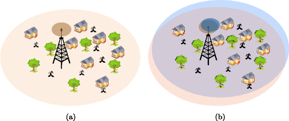
Configurations assumed for the radio access network with one and two carriers, respectively. a Configuration #1. b Configuration #2
-
Configuration #2: a single SC with two carriers with overlapped coverage areas.

Configuration #2 will be required in scenarios where the radio resources of one carrier are not enough to serve the expected traffic during the full day with a given maximum blocking probability. As population density in isolated rural areas is expected to be low and concentrated in a small geographical area, it is assumed that at most two carriers will have enough available resources to serve all generated traffic. Note, however, that the methodology presented in this paper could be generalized to any number of carriers deployed at the same SC. In this configuration, we assume that no interference is produced among communications assigned to different carriers since they use different frequencies, that is, the only interference is coming from communications in the same carrier. However, there are other works in the literature dealing with network planning that consider also inteference from other cells, such as [20], although this lies out of the scope of this paper.
2.2 Traffic model
Voice calls are delivered using the same UMTS service with instantaneous rate R v for all connections. The generation of voice call per user fits a Poisson law with an average rate Λ v [calls/s] and an exponential service time characterized by an average value 1/μ v [s], both for UL and DL.
For radio network dimensioning, we assume that all data traffic is delivered using the same UMTS serviceFootnote 3 with instantaneous rate R d for all connections. File Transfer Protocol (FTP) model 2 [7] is assumed for data traffic characterization, where the requests for data connections are generated following a Poisson law with an average rate Λ d [connections/s] and an exponential service time characterized by an average value 1/μ d [s]. Both Λ d and μ d can be different for UL and DL.
The average rates of generation of voice calls and data connections are time varying functions: Λ v(h) and Λ d(h), where h denotes the hour of the day. A further description of these traffic models can be found in [19].
The average aggregated voice and data connection rates are denoted by λ v(h) and λ d(h), respectively: they are the generation rates multiplied by the number of users (N U ), i.e., λ v(h)=N U Λ v(h) and λ d(h)=N U Λ d(h).
3 Access network dimensioning
This section describes a procedure for the dimensioning of the access network to meet coverage and QoS constraints in terms of blocking probabilities. In this paper, we independently guarantee a maximum blocking probability for voice and a maximum blocking probability for data connections. Among all the possible solutions that fulfill the QoS requirements, we will select the one that requires the minimum backhaul bandwidth. The procedure will be applied to the two configurations described in Section 2.1. For the network dimensioning, the following steps will be taken:
-
Computing the minimum required power at the carriers (in DL) and the UEs (in UL) that are needed to meet the target QoS (see Section 3.1),
-
Assigning power to the DL common channels to satisfy the coverage requirements (see Section 3.2),
-
Computing the coverage probabilities (see Section 3.3),
-
From the coverage probabilities, computing the voice and data blocking probabilities according to different limits on the simultaneous voice and data connections (see Section 3.4),
-
Computing the required backhaul bandwidth for each limit value (see Section 3.5), and
-
Configuring the limit value (i.e., maximum number of simultaneous voice and data connections allowed) that minimizes the required backhaul bandwidth, subject to the specific QoS restrictions (see Section 3.6).
Previous steps are fully described from Sections 3.1 to 3.6. Finally, in Section 3.7, we describe how to extend the proposed methodology to other reference services different from the one considered.
3.1 Power allocation for traffic channels
The objective of the power control procedure is to minimize the required transmission power while keeping the energy per bit to noise power spectral density ratio (E b /N 0), denoted as γ, above a threshold. The radio link quality requirement will depend on the multipath conditions, UE speed, and block error rate required for each type of connection (see [3] and [21] for more details).
In the UL, the target \(\gamma _{{ji}}^{\text {UL}}\) for the j-th user connected to the i-th carrier can be expressed as
where W is the chip rate, S i is the number of users connected simultaneously to the i-th carrier, P ji is the power transmitted by the j-th UE, G ji is the deterministic equivalent gain between the j-th UE and the i-th carrier which includes the antenna gains and the path loss, X ji is the channel fading gain due to the multipath propagation, R j is the bitrate of the j-th user which depends upon the requested service, v j is the activity factor of such service (fraction of time in which the user transmits data), and \({\sigma _{i}^{2}}\) is the Gaussian noise power at the i-th carrier receiver. Notice that in (1), we have assumed that the instantaneous E b /N 0 is equal to the target. This is optimal in terms of minimizing the transmitted power, being this resource allocation strategy typically used in UMTS deployments [19]. The required average transmission power for the j-th user during the connection, \(\bar {P}_{ji}\), assuming that power control mechanism is able to compensate fast fading fairly well if UE speeds are relatively low, is given by
where \(\mathbb {E}[\cdot ]\) denotes the mathematical expectation, \(\mathbb {E}\left [\frac {1}{X_{{ji}}}\right ]\) is the power rise in the UL connection [21], and \(\eta ^{\text {UL}}_{i} = \sum _{s=1}^{S_{i}} \left (1 + \frac {W}{v_{s} R_{s} \gamma _{si}^{\text {\tiny UL}}} \right)^{-1}\) is called the UL load factor [19]. We will assume the same statistical multipath conditions for all UL, i.e., \(\mathbb {E}\left [\frac {1}{X}\right ] = \mathbb {E}\left [\frac {1}{X_{{ji}}}\right ], \,\forall j,i\), and also for the DL, from now on.
In the DL, the link quality expression for the j-th UE connected to the i-th carrier is given by
where \(P^{\text {Ca}}_{i}\) is the total power transmitted through the i-th carrier, \({\sigma _{j}^{2}}\) is the Gaussian noise power at the j-th user, and α j is the orthogonality factor due to the multipath propagation [22]. Notice that we have also assumed here that the instantaneous E b /N 0 is equal to the target for the optimum power allocation. The total power transmitted through the i-th carrier will be \(P_{i}^{\text {Ca}} = P_{i}^{\text {cCH}} + \sum _{s=1}^{S_{i}} P_{is}\), where \(P_{i}^{\text {cCH}}\) is the fixed transmission power intended for the DL common channels and whose value is to be calculated as explained in the following subsection. The average total power transmitted by the carrier i is
where \(\eta ^{\text {DL}}_{i} = \sum _{s=1}^{S_{i}} \left (1 + \frac {W}{v_{s} R_{s} \gamma _{{is}}^{\text {\tiny DL}} \left (1 - \alpha _{s} \right)} \right)^{-1}\) is called the DL load factor [19].
Notice that R j =R v or R j =R d depending on whether the j-th user requests a voice or a data service, respectively. Each service will demand a different target E b /N 0.
3.2 Power allocation for the DL common channels
The power of the DL common channels should be dimensioned to be as low as possible subject to a given quality constraint in the geographical region to be covered. The quality requirement for the common pilot channel (CPICH) can be found in the 3GPP specifications [23, 24], usually in terms of a minimum E c /I 0 (expressed as γ cpich), where E c is the received energy per chip and I 0 is the total received power spectral density at the UE. The quality requirement must be fulfilled in the worst case, corresponding to the user position with the maximum path loss when the carrier is transmitting at maximum power (maximum intra-cell interference). Anyway, for synchronization purposes, the resulting power for the pilot channel must be at least the 5% of the total carrier power [24].
Let \(P^{\text {Ca}}_{\max }\) denote the maximum power transmitted by the i-th carrier. Then, we need to find the minimum required power intended for all the DL common channels, denoted by \(P_{i}^{\text {cCH}}\), such that the following condition is satisfied:
where the subscript p denotes a user located at the worst position within the cell. Given that, the minimum acceptable value of \(P_{i}^{\text {cpich}}\) can be computed as
The total power intended for all the DL common channels, \(P_{i}^{\text {cCH}}\), can be determined by just defining the typical power levels for the rest of the DL common channels in relative terms with respect to the CPICH power [3, 4].
3.3 Coverage probabilities
In this paper, we define the voice and data coverage probabilities, both for the UL and the DL, as the probability of having enough power to accommodate a new incoming voice or data connection request, respectively, given that n voice and m data users are being served simultaneously. These probabilities reflect the fact that there will be users’ positions for which the requests cannot be served due to the lack of available power at the UEs (UL) or carriers (DL).
Coverage probabilities depend on the geographical distribution of the users in the region and the particular geography of the scenario (mountains, rivers, etc.). They cannot be evaluated analytically since, different from urban areas, the density of population is low and the user distribution in the coverage area cannot be considered uniform. However, we can estimate the probability of being able to serve n voice and m data connections simultaneously, which will be denoted as \(P_{n,m}^{\text {cov}}\), through numerical Monte Carlo simulations. To compute these probabilities, random user positions are generated according to a given user distribution modelFootnote 4 corresponding to the concrete geographical area. For each random realization of users’ positions obtained from the user distribution, we compute the transmission powers according to (2) and (4), and finally, we count the number of coverage blocking situations, i.e., the number of realizations for which there is not enough power to fulfill all the link quality requirements.
In the UL, we consider a coverage blocking situation when, at least, one UE does not have enough power to achieve the target \(\gamma _{ji}^{\text {UL}}\), that is,
where \(P^{\text {UE}}_{\max }\) is the maximum available power at the UE, and the Power Control Headroom (PCH) defined in [21] guarantees that the link quality is above \(\gamma _{{ji}}^{\text {UL}}\) during a given fraction of time.
In the DL, a coverage blocking situation occurs when a carrier does not have enough power to ensure the target \(\gamma _{ij}^{\text {DL}}\) for all connections, that is,
where now PCH will depend on the number of simultaneous connections in the cell because the power is shared among them [21].
Finally, from Bayes’ rule, the coverage probabilities are computed as
where \(P_{n\rightarrow n+1,m}^{\text {cov}}\) and \(P_{n,m\rightarrow m+1}^{\text {cov}}\) are the probabilities that given that n voice and m data users are being served simultaneously, there will be enough power to accommodate a new incoming voice or data connection request, respectively.
Notice that for configuration #2, the coverage probabilities will practically be the same for both carriers since the coverage areas fully overlap and they do not interfere with each other.
3.4 Blocking probabilities
Generally, a new voice or data connection request can be accommodated as long as the following two conditions are satisfied simultaneously:
-
1.
There is enough power to fulfill the target link quality requirements. A blocking due to power shortage will be called soft-blocking. Notice that this is related to the coverage probabilities described in Section 3.3.
-
2.
There are free connection resources at a given carrier for the new incoming connection request. A blocking due to the lack of free connection-resources will be called hard-blocking. In practice, the network operator can configure the maximum number of simultaneous connections that the SC can support. According to this, a hard-blocking will occur when a new connection request cannot be processed because the maximum number of simultaneous connections has already been reached.
Note that both soft-blocking and hard-blocking have to be introduced since base stations are limited both in terms of transmission power and the maximum number of simultaneous connections that can be handled, respectively.
In this work, we assume that no queues are available and, therefore, the voice and data blocking probabilities are defined as the probabilities that a new incoming voice or data connection request, respectively, cannot be attended by the network because of having soft-blocking and/or hard-blocking. Note that, since the maximum powers radiated by the SCs and the UEs are low, the probability of having a soft-blocking is not negligible. On the other hand, the hard-blocking cannot be neglected neither, as a limitation on the number of simultaneous connections will be imposed by configuration to minimize the required backhaul bandwidth. Thus, in order to evaluate the blocking probabilities, a joint analysis considering both soft- and hard-blocking has to be carried out.
For the two configurations considered in Section 2, now we derive the expressions of the voice and data blocking probabilities. These expressions are valid both for the UL and the DL. In the following, let C T denote the maximum number of simultaneous connections (voice or data) supported by the carrier, which is a parameter that depends on the SC equipment. At the same time, let \(\hat {C}_{\text {v}}\) and \(\hat {C}_{\text {d}}\) be the maximum number of voice and data connections allowed, respectively. The values of \(\hat {C}_{\text {v}}\) and \(\hat {C}_{\text {d}}\) can be configured by the network operator, and the objective of this paper is to derive the optimum configuration.
3.4.1 Configuration #1
In the case of a single carrier, the blocking probabilities can be evaluated by means of a 2D M/M/m/m Markov chain, where the two dimensions are associated with the number of voice (n) and data (m) connections being active simultaneously at a given instant. Accordingly, the set \(\mathcal {S}(\hat {C}_{\text {v}},\hat {C}_{\text {d}})\) is composed of all possible states detailed as follows (see examples of this set in Fig. 2):

Examples of the allowed states from the 2D M/M/m/m Markov chain. a Case where \(\hat {C}_{\text {v}} + \hat {C}_{\text {d}} \leq C_{\text {T}}\). b Case where \(\hat {C}_{\text {v}} + \hat {C}_{\text {d}} > C_{\text {T}}\)
The shape of this set depends on whether \(\hat {C}_{\text {v}} + \hat {C}_{\text {d}} \leq C_{\text {T}}\) or \(\hat {C}_{\text {v}} + \hat {C}_{\text {d}} > C_{\text {T}}\) (see Fig. 2). Now, let us define the following four disjoint subsets, \(\mathcal {A}_{i}\left (\hat {C}_{\text {v}},\hat {C}_{\text {d}}\right) \subseteq \mathcal {S}\left (\hat {C}_{\text {v}},\hat {C}_{\text {d}}\right)\), such that \(\bigcup _{i=1}^{4} \mathcal {A}_{i}\left (\hat {C}_{\text {v}},\hat {C}_{\text {d}}\right) = \mathcal {S}\left (\hat {C}_{\text {v}},\hat {C}_{\text {d}}\right)\):
The subset \(\mathcal {A}_{1}\) is composed of the states in the slope border (if \(\hat {C}_{\text {v}} + \hat {C}_{\text {d}} > C_{\text {T}}\)) or only of the top-right corner state (if \(\hat {C}_{\text {v}} + \hat {C}_{\text {d}} \leq C_{\text {T}}\)). \(\mathcal {A}_{2}\) and \(\mathcal {A}_{3}\) contain the states in the vertical and horizontal border, and finally, \(\mathcal {A}_{4}\) is composed of all non-border states. The links between the states are illustrated in Fig. 3, where

Examples of the allowed states of the 2D M/M/m/m Markov chain
Notice that not all the states will have all the possible outgoing and ingoing links. For example, blue links will not exist if \((n,m) \in \mathcal {A}_{2}\), red links will not exist if \((n,m) \in \mathcal {A}_{3}\), and neither blue nor red link will exist if \((n,m) \in \mathcal {A}_{1}\).
The state probabilities, \(\left \{\hat {P}_{n,m} (\hat {C}_{\text {v}},\hat {C}_{\text {d}}), \, \,(n,m) \in \mathcal {S}(\hat {C}_{\text {v}},\hat {C}_{\text {d}}) \right \}\), which obviously also depend on the pair \((\hat {C}_{\text {v}},\hat {C}_{\text {d}}) \), need to be calculated numerically by adopting the theory of stationary continuous Markov chains. This allows assessing that the probability of reaching any state can be computed from the probability of the neighbor states and the transition rates [25].
The voice (\(\hat {P}_{\text {C}}^{\text {v}}\)) and data (\(\hat {P}_{\text {C}}^{\text {d}}\)) congestion probabilities are the probabilities of having a hard-blocking. This happens if the SC is already serving the maximum number of users supported (C T) or the maximum number of voice or data connections set by the network operator (i.e., \(\hat {C}_{\text {v}}\) and \(\hat {C}_{\text {d}}\), respectively). Thus, they can be expressed as
Finally, the voice (\(\hat {P}_{\text {B}}^{\text {v}}\)) and data (\(\hat {P}_{\text {B}}^{\text {d}}\)) blocking probabilities are given by
Note that these probabilities are the sum of the probability of having a hard-blocking (congestion probability) and the probability of having a soft-blocking. In other words, (20) and (21) are the probabilities that a new incoming voice or data connection request cannot be accommodated since there is not enough power at the transmitter and/or because the maximum number of simultaneous connections has been reached.
3.4.2 Configuration #2
When two carriers are active (namely carriers A and B), the voice and data blocking probabilities can be evaluated through a 4D M/M/m/m Markov chain. Its dimensions are associated with the number of voice (n) and data users (m) connected to carrier A and the number of voice (k) and data users (l) connected to carrier B at a given instant, where each state is denoted by (n,m,k,l). We assume that both carriers are able to support the same maximum number of simultaneous connections (C T). In the construction of the chain, we consider that one UE attempts to connect to one carrier or the other one with equal probability and, if one carrier cannot provide service, then the corresponding connection request is forwarded to the other carrier. In this situation, a request will be disregarded only if none of both carriers are able to accommodate itFootnote 5.
Let \(\hat {C}^{A}_{\text {v}}\), \(\hat {C}^{A}_{\text {d}}\), \(\hat {C}^{B}_{\text {v}}\), and \(\hat {C}^{B}_{\text {d}}\) denote the maximum numbers of simultaneous connections for voice and data users allowed at carriers A and B, respectively (where these values are to be configured by the network operator). Then, the set \(\mathcal {S}\) of all possible states is:
Now, we define the following non-disjoint subsets \(\mathcal {A}_{i}\left (\hat {C}^{A}_{\text {v}},\hat {C}^{A}_{\text {d}},\hat {C}^{B}_{\text {v}},\hat {C}^{B}_{\text {d}} \right) \subseteq \mathcal {S}\left (\hat {C}^{A}_{\text {v}},\hat {C}^{A}_{\text {d}},\hat {C}^{B}_{\text {v}},\hat {C}^{B}_{\text {d}} \right)\), such that
where
The links between the states are depicted in Fig. 4. Some of them will be different depending on the subset where the states belong to. Thus, for the two subsets where both carriers are not serving the maximum number of voice or data connections (\(\mathcal {A}_{7}\) or \(\mathcal {A}_{8}\), respectively), the rates for the transitions can be derived assuming that voice and data traffic spill between carriers is possible:

Examples of the allowed states of the 4D M/M/m/m Markov chain
Note that \((n,m,k,l) \in \mathcal {A}_{7}\) includes implicitly some states that are also in \(\mathcal {A}_{2}\), \(\mathcal {A}_{5}\), and \(\mathcal {A}_{6}\) due to the fact that the subsets \(\left \{ \mathcal {A}_{i}\right \}_{i=1}^{8}\) are not disjoint. The same applies for \(\mathcal {A}_{8}\), which includes some states that are also in \(\mathcal {A}_{1}\), \(\mathcal {A}_{3}\), and \(\mathcal {A}_{4}\).
For the subsets where one carrier is serving the maximum number of voice or data connections (\(\mathcal {A}_{3}\) and \(\mathcal {A}_{4}\), or \(\mathcal {A}_{5}\) and \(\mathcal {A}_{6}\), respectively), traffic spill is not possible, and therefore, we have
Note again that for example, \(\mathcal {A}_{3}\) includes some states that are also in \(\mathcal {A}_{2}\), \(\mathcal {A}_{5}\), \(\mathcal {A}_{6}\), and \(\mathcal {A}_{8}\).
As happened before, the state probabilities \(\hat {P}_{{n,m,k,l}}\big (\hat {C}^{A}_{\text {v}},\hat {C}^{A}_{\text {d}},\hat {C}^{B}_{\text {v}},\hat {C}^{B}_{\text {d}} \big)\), for \((n,m,k,l) \in \mathcal {S} \big (\hat {C}^{A}_{\text {v}},\hat {C}^{A}_{\text {d}},\hat {C}^{B}_{\text {v}},\hat {C}^{B}_{\text {d}} \big)\) cannot be obtained in closed form [25]. In order to calculate them, first, the voice and data congestion probabilities can be computed as
Accordingly, the final expressions for the blocking probabilities are
If more than two carriers were considered, the previous analysis could be generalized by augmenting the dimensionality of the Markov chains accordingly (if p carriers with overlapping coverage areas are assumed, then 2p-dimensional M/M/m/m Markov chains should be handled).
3.5 Backhaul bandwidth calculation
In this section, we introduce the procedure to compute the required backhaul bandwidth for given \((\hat {C}_{\text {v}},\hat {C}_{\text {d}})\) in configuration #1 and \((\hat {C}^{A}_{\text {v}},\hat {C}^{A}_{\text {d}},\hat {C}^{B}_{\text {v}},\hat {C}^{B}_{\text {d}})\) in configuration #2. Let f be an increasing function that maps the number of simultaneous connections into the required backhaul bitrate. For example, f could be a linear function such as f(n,m,k,l)=(a+1)(n+k)R v+(b+1)(m+l)R d, where a and b are the fraction increase of the voice and data backhaul bitrate per access network connection due to the backhaul overhead, respectively. If compression schemes are implemented, then the required backhaul bitrate may not increase linearly with the number of connections, as assumed in [19].
The backhaul bandwidth should be able to accommodate the largest bitrate generated by the access network. If data connections require more bandwidth than voice connectionsFootnote 6, then the state that requires the largest backhaul bandwidth for configuration #1, denoted as (n ′,m ′) will be
For configuration #2, the state that generates the largest backhaul rate, denoted as (n ′,m ′,k ′,l ′), according to the quadruple \((\hat {C}^{A}_{\text {v}},\hat {C}^{A}_{\text {d}},\hat {C}^{B}_{\text {v}},\hat {C}^{B}_{\text {d}})\) is
The minimum required backhaul rate \(\hat {T}_{\text {T}} \left (\hat {C}_{\text {v}},\hat {C}_{\text {d}} \right)\) in configuration #1 is
and the required backhaul rate \(\hat {T}_{\text {T}} \left (\hat {C}^{A}_{v},\hat {C}^{A}_{d},\hat {C}^{B}_{v},\hat {C}^{B}_{d} \right)\) in configuration #2 is
3.6 Network dimensioning methodology
The state probabilities of the Markov chain in the previous section depend on the limit imposed to the number of simultaneous of voice and data connections (i.e., \(\hat {C}_{\text {v}}\) and \(\hat {C}_{\text {d}}\) that are parameters to be configured by the network operator) and also on the average aggregated rates of incoming voice and data connection requests (i.e., λ v and λ d). If these rates are not constant throughout the day, then the blocking probabilities and the required backhaul bandwidth will depend on the quadruple \((\hat {C}_{v}, \hat {C}_{d}, \lambda _{\text {v}}(h), \lambda _{\text {d}}(h))\) for configuration #1, and on the sextuple \( (\hat {C}^{A}_{v}, \hat {C}^{A}_{d}, \hat {C}^{B}_{v}, \hat {C}^{B}_{d}, \lambda _{\text {v}}(h), \lambda _{\text {d}}(h))\) for configuration #2.
Let us assume that the voice service uses spreading codes with a spreading factor F v, then the maximum number of voice connections in the DL will be N= min(C T,F v). For data services with a spreading factor F d, the maximum number of data connections in the DL will be M= min(C T,F d). In the UL, the limitation imposed by the spreading factor does not exist [4] and, therefore, the maximum number of voice and data connections in the UL will be directly N=C T and M=C T, respectively.
For configuration #1, the dimensioning requires the numerical evaluation of the backhaul bandwidth \(\hat {T}_{\text {T}} \left (\hat {C}_{\text {v}},\hat {C}_{\text {d}} \right)\) considering that the voice and data blocking probabilities must be below a given threshold, i.e., \(\hat {P}^{\text {v}}_{\text {B}} (\hat {C}_{\text {v}}, \hat {C}_{\text {d}}, \lambda _{\text {v}}(h), \lambda _{\text {d}}(h)) \leq \Gamma _{\text {B}}^{\text {v}}\) and \(\hat {P}^{\text {d}}_{\text {B}}(\hat {C}_{\text {v}}, \hat {C}_{\text {d}}, \lambda _{\text {v}}(h), \lambda _{\text {d}}(h)) \leq \Gamma _{\text {B}}^{\text {d}}\), where \(\Gamma _{\text {B}}^{\text {v}}\) and \(\Gamma _{\text {B}}^{\text {d}}\) are the target blocking probabilities. This condition must be fulfilled for all hours of the day. Note that the evaluation of each new pair \((\hat {C}_{\text {v}}, \hat {C}_{\text {d}})\) implies to construct a new Markov chain with different states; hence, no closed-expression exists for \(\hat {T}_{\text {T}} \left (\hat {C}_{v},\hat {C}_{d}\right)\). The configuration corresponding to the values of \(\hat {C}_{v}\) and \(\hat {C}_{d}\) that requires least bandwidth is finally chosen. The proposed methodology is described in Table 1.
The methodology for configuration #2 can be derived similarly to the previous one. For the sake of clarity in the presentation, this methodology is summarized in Table 7 in Appendix 2 and provides the optimum limit on the number of simultaneous voice and data connections to be configured for each carrier. Furthermore, the procedure presented in this section is valid both for the UL and the DL.
3.7 Network dimensioning beyond UMTS
In the previous sections, we have presented a methodology for the dimensioning of a network in rural areas. To describe the methodology in a simple and illustrative way, we have considered UMTS as the reference service. As already explained, the so designed network will be able to operate satisfactorily with the reference service considered as well as with any other service that makes a more efficient usage of the network resources.
It is important to emphasize that in case that another reference service is to be considered in the dimensioning, the same methodology could be applied accordingly after computing the new coverage probabilities and restructuring the multidimensional Markov chains. For instance, if, in order to avoid overprovisioning of network resources, High-Speed Packet Access (HSPA) is considered, the following aspects should be taken into account:
-
The HSPA rates depend on the instantaneous channel conditions;
-
HSPA rates in a multi-user setup depend also on the concrete scheduling strategy considered.
For a simple round robin scheduling strategy, the states in the Markov chains should include information regarding the rate of each data connection (which in turn depends on the instantaneous channel states). Even if the user’s data rates are restricted to a set of Q discrete possible values, the number of states in the Markov chains would increase proportionally to Q to the number of connections. Note that the analysis would be valid only for the concrete scheduling considered. Logically, if the adopted scheduler in the network is more efficient, the performance of the network would meet (and even surpass) the target QoS considered at the network dimensioning stage.
Also, the methodology could be extended to incorporate different admission control strategies. For example, if voice connections had priority over data connections, then the Markov chains should be redefined accordingly by creating new archs from those states in which the maximum number of voice connections have been reached. Those archs would model the fact that if a new voice connection request arrives, one data connection should be interrupted to attend the voice connection. Another possibility would be, in this case, not to interrupt any data connection, but to reduce the rate of all the data connections in order to release resources to be able to serve the voice connections. This last option would imply defining new states in the Markov chain. Anyway, the conclusion is that the methodology that we present would be the same and that it could be adapted properly to the concrete scheduling, admission control, etc. schemes that are to be considered as a reference service.
When considering other technologies, such as 4G and 5G, the steps described in the proposed methodology (see Fig. 5) can still be applied with proper adaptations. In particular, the power allocation expressions should be adjusted by considering the specific signal-to-interference plus noise ratio (SINR) of the technology considered. In some cases, the skeleton of the Markov chains should also be adapted to the specific reference service, admission control, and scheduler.

Methodology presented in the paper to carry out the network dimensioning

Traffic intensity distribution and coverage probability. a Traffic intensity. Traffic intensity in yellow areas corresponds to half the intensity in white areas. The traffic intensity in green areas is considered negligible. The absolute values of the generated traffic depend on the time instant and the year, as explained in the paper and illustrated through numerical examples in the simulations section. b Coverage probability of being able to attend n voice and m data users simultaneously, in other words, probability that there is enough transmit power to be able to attend this number of connections simultaneously. This probability depends on the spatial distribution of users according to figure above. The colors refer to the values of this probability according to the right vertical colorbar
4 Energy provision and energy systems dimensioning
The goal of this section is to determine the number of required solar panels and batteries denoted as n SP and n B , respectively, to provide energy to the SC.
4.1 Energy computation
Let us consider initially only one carrier (i.e., configuration #1), the maximum number of simultaneous voice and data connections is (C v,C d), and all possible states of the Markov chain define the region \(\mathcal {S}\). Since λ v(h) and λ d(h) vary over the day, the state probabilities will also be time varying functions, denoted as P n,m (h). Now, let f(P R |n,m) denote the probability density function (PDF) of the power radiated (P R ) by the carrier conditioned to having n voice and m data simultaneous active connections. Notice that \(f\left (P_{R} | n,m \right), \forall (n,m)\in \mathcal {S}\) should be obtained through Monte Carlo simulations since an analytical expression does not exist. Therefore, the PDF of the total radiated power conditioned to a particular hour of a day can be expressed as
and the average power radiated by the carrier in one particular hour is given by
In order to dimension the energy units, we need to model the total power consumption. The power consumption model by [26] is:
where P max is the maximum radiated power, P 0 is a fixed power consumption of the equipment that models the radio frequency (RF) and baseband consumptions, and Δ p is a constant. For the moment, we do not consider the consumed power when the carrier is switched off (given by P sleep). Given that, the total average energy consumption (in W h) is
If the two carriers are switched on (i.e., configuration #2), the state probabilities are denoted as P n,m,k,l (h). The PDF of the total radiated power conditioned to a particular hour of a day can be expressed as
where f(P R |n,m,k,l) denotes the PDF of the power radiated by the SC when serving n and k voice, and m and l data simultaneous connections at both carriers. Then, the average energy consumption can be computed using (43).
4.2 Energy dimensioning
The energy dimensioning procedure followed in this work is based on [27]. The total energy that the solar panels should generate within one day is:
where η G denotes the losses due to the inefficiency of the solar cells (around 10% [27]), L is the total energy spent within one day (calculated following (43)), and f c is a correction factor (f c =1.3 [27]) introduced as the solar cells have to generate energy for the batteries and the panels themselves to be able to work. The number of solar panels depends on the solar radiation in the place of interest and nominal power of the solar cell, P nom, which is obtained assuming that solar radiation is 1000 W/m2. Given that, the number of solar panels needed is
where G dm is usually taken as the average daily solar radiation during the worst month of the year. The capacity of the batteries (in W ·h) should be enough to provide electrical energy during up to N da days without any charging procedure. Therefore, the capacity of the batteries must satisfy
where \(P^{d}_{\text {max}}\) is a parameter to impose that a battery should have at least 20% of its maximum capacity (\(P^{d}_{\text {max}}=0.8\)).Footnote 7 Finally, if C 1 is the capacity of a single battery, the number of required batteries becomes
where ⌈·⌉ is the ceiling operator.
5 Carrier on/off switching strategies
In this section, we introduce a technique to dynamically switch on and off one of the two carriers in locations where the configuration #2 is needed. The goal is to reduce as much as possible the energy consumption. Consider, for example, a situation where all the traffic could be served with just one carrier, but it could happen that in order to compensate the intra-cell interference, two carriers would require less power to serve this traffic (we also have to take into account that the carrier has a fixed power consumption due to the electronic equipment, as modeled by the term P 0 in (42)). Thus, if the power increase to overcome interference is higher than the fixed power consumption of the carrier, then, the configuration with two carriers would be optimal in terms of energy reduction. This is just an example, but other situations may be possible.
To determine whether a carrier should be switched off or not, we need to measure and compare the required power that is needed for both configurations (i.e., one or two carriers), to serve the users with a specific traffic demand. This power can be obtained through simulations for each hour of the day.
We will derive two approaches: a deterministic approach considering full knowledge of the traffic profile throughout the day, and a statistical robust strategy accounting for error traffic modeling. For the deterministic procedure, we develop a method that assumes either a single type of traffic (voice) or mixed traffic (voice and data). The decision of switching on and off carriers will be based on a threshold applied to the traffic demand at each hour of the day.
Although this paper deals with two possible states (“on” and “off”) and two carriers, the methodology could be adapted to more flexible configurations. For example, if a more accurate description of the energy consumption is to be incorporated, then more than two possible states of the carriers should be defined (e.g., idle, waking up, sleep entering, active (data), active (signaling), sleep, etc.), each of them with different energy profiles. It has also to be emphasized that the transition times between these states may be different, which should be considered when defining the corresponding Markov chains that would be more complicated. Chung [28] considers this and models the transitions among states through a semi-Markov process approach. Also, if more than two carriers are considered, the dimension of the Markov chains would increase up to twice the number of carriers and the strategy that will be presented in this section should include multiple thresholds on the traffic intensity, each one defining when a new carrier should be activated or deactivated. Anyway, for the sake of simplicity, we keep our analysis assuming two carriers and two possible states since the proposed methods and concepts would remain the same even if more complicated and flexible configurations are to be considered. In other words, the focus of this paper is on the methodology that is the same regardless the number of states and carriers and, therefore, the corresponding Markov chains.
5.1 Deterministic switching strategy
5.1.1 Single type of traffic
In this first approach, we assume just voice connection requests and that the rate of requests is completely known over the day. In order to be more realistic, we consider discretized traffic profiles. Accordingly, let λ 0v [m] represent the rate of connection requests (in requests/second) corresponding to the m-th time instant within the day (the decision to switch on and off the carrier can only be taken at predetermined time instants). This corresponds to the discretized version of the aggregated continuous voice call generation rate λ v(h). In Table 2, we present the procedure to calculate the threshold λ TH to be applied to λ 0v [m] for switching on/off a carrier in this case. Basically, the method described in this table to calculate the threshold evaluates if the traffic demand can be served by one carrier or two carriers. In case that one carrier is not enough, then two carriers are activated. Otherwise, if both configurations are possible, then the algorithm selects the configuration which requires less power.
5.1.2 Two types of traffic
We consider now voice and data traffic, whose rates of connection requests are denoted by λ 0T [m]=(λ 0d [m],λ 0v [m]) (as done before, we consider a discrete-time approach). Note that λ 0d [m] is different for the UL and the DL, but we assume that the energy spent in UL processing is incorporated in the constant component of (43) and does not affect the radiated power. Therefore, we will only consider the DL λ 0d [m] to design the switching threshold. In Table 3, we present the procedure to calculate the threshold frontier λ TH to decide whether for a given traffic λ 0T [m], we have to switch on or off a carrier. Now, the threshold λ TH is a frontier in a two-dimensional plane composed of tuples of voice and data traffic demands, (λ 0d , λ 0v ). Similarly to the previous case of one type of traffic, here the method to calculate the threshold frontier evaluates if the traffic demand can be served with one or two carriers. If one carrier is not enough, then two carriers are activated. Otherwise, the configuration requiring less power is selected.
5.2 Robust switching strategy
In the previous subsection, we considered that the value of the traffic generation rate was perfectly known. However, in some situations, it is very difficult to obtain such information with a high precision. For already deployed networks, measurements campaigns can be performed to obtain the traffic profile throughout the day. Nevertheless, the expected value of traffic is something that is not stable and depends on the specific location, unexpected events, or even the particular day of the week. As a consequence, slight variations of the nominal traffic profile will be experienced. On the other hand, in locations where the network is not already deployed, the uncertainty is even higher since network planning engineers usually assume a nominal traffic of a similar already deployed network elsewhere. This implies a risk that such traffic information is not an accurate approximation of the actual one. For these reasons, we propose a new model to cope with such uncertainties and make the final switching procedure robust against them. For simplicity in the notation and the mathematical developments, we will consider only one type of traffic but a possible extension to mixed traffics is presented later on.
Let us consider that the traffic profile is a stochastic discrete process modeled as a deterministic mean plus a random component:
where λ 0[m] corresponds to the available nominal profile and p[m] is a zero mean white Gaussian process with variance \({\sigma _{p}^{2}}\) (\({\sigma _{p}^{2}}\) may also vary, i.e., \({\sigma _{p}^{2}}[m]\), but for simplicity, we will consider it constant). The process p[m] incorporates all possible uncertainties described before. Gaussianity of this modeling error is not sustained by any observation, but it will provide an approximate way to adjust the switching threshold as a function of the uncertainty level.
The goal of this section is to obtain a new threshold for switching on/off the carriers fulfilling a given predetermined target outage probability. The decision of shutting down the carrier will be based on the comparison of an estimate of λ[m] with the new threshold. In order to estimate the traffic being generated, we define a time window where we will measure it. Let M be the number of time instants that are considered for measuring the traffic and T be the time lapse between consecutive time instants. The reason why M time instants are used instead of just one is the stabilization of the estimate of the generated traffic, that is, to reduce the variance of the estimation. Let us consider the following definition:
where \(\bar {p}_{t} \sim \mathcal {N}(0,\bar {\sigma }_{p}^{2}), \,\, \bar {\sigma }_{p}^{2} = MT^{2}{\sigma _{p}^{2}}\). In order to avoid \(\bar {\lambda }_{t}\) being negative, we truncate the Gaussian distribution of \(\bar {p}_{t}\) in a way that \(-\bar{\lambda}_{0t} < \bar {p}_{t} < \infty \). Then, \(\bar {p}_{t}\) has a truncated normal distribution with PDF given by
where \(\Phi _{t} \triangleq \frac {1}{\sqrt {2\pi }\bar {\sigma }_{p}}\int _{-\bar {\lambda }_{0t}}^{\infty }\text {e}^{-\frac {s^{2}}{2\bar {\sigma }_{p}^{2}}}\,\text {d}s\).
5.2.1 Traffic profile estimation
Let us consider N measurements (obtained, for example, from N previous days) of the number of connection requests, denoted as k tn , n=1,…,N, during the same time period to estimate \(\bar {\lambda }_{t}\) (k tn represents the number of connection requests measured within the time window [t,t+M−1] of the day n). We know that such variable is Poisson distributed where the probability of a given value of k tn is given by \(\text {Pr}(k_{tn}) = \prod _{n=1}^{N} \text {e}^{-\bar {\lambda }_{t}}\frac {(\bar {\lambda }_{t})^{k_{tn}}}{k_{tn}!}\). We formulate the maximum likelihood (ML) estimator of \(\bar {\lambda }_{t}\) given the N observations \(\{k_{tn}\}^{N}_{n=1}\) as [29]
and
Note that \(\sum _{n=1}^{N} k_{tn}\) is Poisson distributedFootnote 8 with expected value \((\bar {\lambda }_{0t} + \bar {p}_{t})N\).
5.2.2 Threshold computation based on outage probability
Given the previous traffic estimate, the Bayesian robust outage condition \(\bar {P}_{\text {out}}\) is defined as
where \(\bar {\lambda }_{t_{w}} = \bar {\lambda }_{0t_{w}} + \bar {p}_{t_{w}}\), θ is the outage probability with which we tolerate that the carrier is switched off when, in fact, both carriers should be on, \(\bar {\lambda }_{{TH}}^{'}\) is the new threshold to be computed, the expectation is with respect all possible error modeling, and t w is the worst case time instant that defines the time window as
where λ TH is the deterministic threshold found in the previous section. As the outage condition should be fulfilled for the whole traffic profile over the day, we have to find the time window where the estimate \(\hat {\lambda }_{ML}(t)\) will be most susceptible to originate situations where the carrier should be on but the estimate decides to turn it off. This will happen at the worst case time-instant within the day, that is, the instant in which the measurement of the generated traffic is most different from the threshold, as formulated in (55). Notice that a trivial solution is to set \(\bar {\lambda }_{TH}^{'} = 0\). However, in this situation, both carriers will be always on and no energy saving is possible. For that reason, the threshold \(\bar {\lambda }_{TH}^{'}\) should be the maximum value of \(\bar {\lambda }_{TH}^{'}\) that fulfills (54). Note that (54) has a unique solution because it is an increasing monotonic function in \(\bar {\lambda }_{TH}^{'}\) (we are averaging a cumulative distribution function (CDF)). The last step requires the normalization \(\lambda _{TH}^{'} = \frac {\bar {\lambda }_{TH}^{'}}{MT}\) to get units of number of connection requests/s. Let us present the following result:
Proposition 1
The Bayesian outage probability, \(\bar {P}_{\text {out}}\), can be approximated in closed-form solution by the following expression:
where \(\mathcal {Q}(x) = \frac {1}{\sqrt {2\pi }}\int _{x}^{\infty } \text {e}^{\frac {u^{2}}{2}}\,\text {d}u\) is the Gaussian \(\mathcal {Q}\)-function [30], \(x = \lceil \bar {\lambda }_{TH}^{'} N\rceil +1\), \(\mathrm {\Gamma }(x)= \int _{0}^{\infty } s^{x-1} \text {e}^{-s}\,\text {d}s\) is the Gamma function [31], \(\gamma (n,x)= {\int _{0}^{x}} s^{n-1} \text {e}^{-s}\,\text {d}s\) is the lower incomplete Gamma function [31], \(\Delta _{1} = \frac {1}{\sqrt {\pi }}\int _{\bar {\lambda }_{0}}^{\infty }\text {e}^{-(m-\mu _{1})^{2}}\,\text {d}m\), \(\Delta _{2} = \frac {1}{\sqrt {\pi }}\int _{\bar {\lambda }_{0}}^{\infty }\text {e}^{-(m-\mu _{2})^{2}}\,\text {d}\bar {m}\), \(\Delta _{3} = \frac {1}{\sqrt {\pi }}\int _{0}^{\bar {\lambda }_{0}}\text {e}^{-(m-\mu _{1})^{2}}\,\text {d}\bar {m}\), \(\Delta _{4} = \frac {1}{\sqrt {\pi }}\int _{0}^{\bar {\lambda }_{0}}\text {e}^{-(m-\mu _{2})^{2}}\,\text {d}\bar {m}\), \(K = \frac {1}{(x-1)!\Phi _{t_{w}}}\), \(K_{1} = \frac {N^{x}\text {e}^{-N\bar {\lambda }_{0t_{w}}+N^{2}\bar {\sigma }^{4}_{p}}\sqrt {\pi }}{12(x-1)!\Phi _{t_{w}}}\), \(K_{2} = \frac {N^{x}\text {e}^{-N\bar {\lambda }_{0t_{w}}+\frac {9N^{2}\bar {\sigma }^{4}_{p}}{16}}\sqrt {\pi }}{4(x-1)!\Phi _{t_{w}}}\), \(\mu _{1} = -(\bar {\sigma }_{p}^{2}N-\bar {\lambda }_{0t_{w}})\), \(\mu _{2} = -\left (\frac {3\bar {\sigma }_{p}^{2}N}{4}-\bar {\lambda }_{0t_{w}}\right)\), and Ψ(·) is the moment of a truncated Gaussian variable as defined in Appendix 3.
Proof
See Appendix 4. □
5.2.3 Extension to two types of traffic
Previously, we assumed for the Bayesian robust threshold that there was only one type of traffic or, equivalently, that there were two types of traffic and that the load corresponding to one of them was known without uncertainty. In case that the traffic loads for both kinds of traffic are known imperfectly, we should define a robust Bayesian threshold frontier by means of extending the previous integrals to include simultaneously the uncertainty model for both traffics. Such integrals are, however, extremely complicated and have to be solved resorting to complex numerical methods. A simpler way to derive a suboptimum robust threshold frontier could be based on the following idea:
-
1.
Assuming that the data traffic load is known perfectly, calculate the robust threshold for the voice traffic for each possible value of data traffic load using the methodology presented previously for one kind of traffic.
-
2.
Assuming that the voice traffic load is known perfectly, calculate the robust threshold for the data traffic for each possible value of voice traffic load using the methodology presented previously for one kind of traffic.
-
3.
Combine both thresholds shifts in a vector in a two-dimensional plane.
6 Simulation results
In this section, we provide some numerical results. The setup under consideration is a real scenario that has been designed and planned in the European project TUCAN3G (http://www.ict-tucan3g.eu), taking data from some real rural locations in the Peruvian Amazon.
6.1 Network planning results
As example, we present the planning results for the location of San Gabriel (one of the towns of Perú evaluated in [19]). Figure 6a shows the expected traffic intensity over the geographical area and the position of the telecommunication tower (displayed as a red point). The traffic intensity in yellow areas corresponds to half the intensity in white areas. Voice traffic is served using a rate R v =12.2 kbps and data traffic using a rate R d =128 kbps (the spreading factor for one voice and data connection in the DL is 128 and 16, respectively). The average aggregated rate of connection requests for voice and data at the peak hour are λ v(h peak)=0.0558 and λ d(h peak)=0.2208 connections/s, respectively, in the DL, and λ v(h peak)=0.0558 and λ d(h peak)=0.0736 connection/s in the UL. Note that the peak hours for voice an data traffic need not be the same. The average voice and data service times are 1/μ v=90.09 s and 1/μ d=3.775 s, both for the UL and DL. The specific daily traffic profile was provided by Telefonica del Perú [19]. Traffic intensities are expected to increase by 180% in the second year, by 4% in the third year, and by 2% in the fourth and fifth year after the deployment setup. Carriers can transmit a maxim power of \(P_{\max }^{\text {Ca}}=20\) dBm and support C T=16 maximum simultaneous connections. The antenna gains for the carriers are 7 dB. The backhaul bitrates according to the number of voice and data connections are displayed in Fig. 7a, b, respectively. The characterization of the radio link budget parameters can be found in [19].

Backhaul bitrates for voice and data connections. a Backhaul bitrates according to the number of voice connections. b Backhaul bitrates according to the number of data connections
The first step in the network planning is to determine the power allocated to the DL common channels. The imposed coverage requirement is that carriers must be capable to cover the 95% of the geographical area considered.
The next step is to compute the coverage probabilities (\(P^{\text {cov}}_{n,m}\)) through Monte Carlo simulations. Figure 6b depicts these probabilities for the DL.
Table 4 displays the optimum limits on the number of simultaneous connections (C v and C d ) and the required backhaul bandwidth to guarantee a maximum blocking probability of 2% for both services. These results are given for the UL and the DL during a period of 5 years, considering one and two carriers. Notice that the required voice channels are the same both for the UL and DL since the voice traffic is expected to be symmetric, whereas the required data channels are higher in the DL because the data connection rate in the DL is three times higher than in the UL. From the second year on, the configuration with only one carrier is not enough to serve all the expected traffic. The values from second year on are quite similar due to the limited traffic growth. Note also that two values for C v and C d are given when two carriers are considered.
6.2 Energy dimensioning results
In this subsection, we provide simulation results for the dimensioning of the energy units and the results of the on/off switching strategy. The considered batteries have the following specifications: 12 V, 100 Ah, and a capacity C 1=1200 Ah × V. The solar panels have a nominal power P nom=85 W. We consider that N da=3 days. In this section, we consider three different maximum radiated powers \(P_{\max }^{\text {Ca}}\) per carrier for three different types of SC (SC a 20 dBm, SC b 13 dBm, and SC c 24 dBm) [19]. We assume that we have four different traffic profiles corresponding to four different rural towns denoted as TP1 (Santa Clotilde), TP2 (Negro Urco), TP3 (Tuta Pisco), and TP4 (San Gabriel), as opposed to the previous subsection where we only considered one town. We also assume that the network dimensioning must be performed considering the traffic estimation forecast for the incoming 5 years (details of the forecast evolution were given in the previous subsection, further details are available in [19]). The parameters of the power consumption model [26] are set to P 0=4.8 W, Δ p =8, and P sleep=2.9 W for the femtocell model and P 0=6.8 W, Δ p =4, and P sleep=4.3 W for the picocell model [26]. The femtocell model is always considered from now on if not stated otherwise.
Let us first present the results for the energy dimensioning units when we have a static design, i.e., when we do not apply any on/off strategy. In this case, the dimensioning is performed considering average consumed power given by (43). Table 5 summarizes the required number of solar panels and batteriesFootnote 9 over the 5 years considering the two consumption models and a maximum radiated power of 20 dBm (i.e., SC a ). Notice that in the first year if the two carriers are always on, the required energy items are almost twice the ones needed when just one carrier is switched on. It means that the consumed energy is highly independent of the radiated power intended to serve traffic as can be seen from (42). This phenomenon can also be seen from the number of required energy units. Again, the values from second year on are similar due to limited traffic growth.
Figure 8 depicts the traffic profile considering only voice for a specific location and the corresponding threshold for switching on/off one of the two carriers. The type of carrier considered is SC a . As we can see, the two carriers are needed only a few hours during the day (30% of the total time). For the rest of the day, one carrier is enough. Thus, potential energy savings can be obtained.

On/off switching threshold example for a single traffic profile during the first year with traffic type TP1
Figure 9 depicts the reduction in the required size of solar panel and the consumed power in percentage compared to the case where two carriers are always active if only voice traffic is considered. The results are represented as a function of the estimated traffic evolution in 5 years for different traffic profiles and different types of carriers. Battery size is linearly proportional to the solar panel size, and thus, the experienced reduction is the same in both cases. As it can be observed, for some traffic profiles the amount of reduction (in CAPEX) is around 15–20% for the first years.

Cost and energy savings for different traffic profiles and different types of carriers within the first 5 years. a Solar panel reduction size. b Power consumption reduction
Figure 10 shows some results for the on/off switching procedure when two types of traffics are considered. Figure 10 a depicts the threshold region determining the tuples of voice and data traffic rates for which one of the carriers can be switched off. Figure 10b depicts the particular hours of the day when this can be done. For the specific traffic profile TP1 and using carrier type SCc, only for 10 h per day, the two carriers are needed during the first year. Figure 10 c depicts the reduction of the solar panel size in percentage if the deterministic on/off strategy is implemented compared to the case where the two carriers are always active for mixed traffic demands. As it can be seen, as the traffic increases during the second year, the configuration with two carriers on is required for more hours during the day and thus, only 5% of saving is possible.

On/off threshold region, hours to be switched off for a specific traffic profile for the first year, and solar panel size reduction for mixed traffic. a Region of lambda threshold for mixed traffic. b On/off threshold example for mixed traffic profile. c Solar panel size reduction for mixed traffic and two different traffic profiles
Figure 11 a shows the threshold computed using the Bayesian robust methodology for a given variance of p[n] and for different outage probabilities θ. We also show the deterministic threshold (when the traffic profile is perfectly known). We can see that, if we allow a higher outage probability, then the threshold increases. For the particular case of θ=0, the threshold should be set to zero, i.e., \(\lambda _{TH}^{'} = 0\). Another effect that we can see, as expected, is that for larger variances, we cannot trust the estimation and, thus, the threshold must be reduced to guarantee the same outage. We also see that for high variances, the outage probability does not have an important impact on the threshold calculation.

Example of on/off switching robust Bayesian threshold for different values of outage probability θ and variance \({\sigma _{p}^{2}}\). For comparison purposes, the deterministic threshold λ TH is also depicted. a Bayesian threshold as a function of the variance \({\sigma _{p}^{2}}\) for different outages. b Bayesian threshold as a function of the outage probability for \({\sigma _{p}^{2}} =0\)
Finally, Fig. 11 b depicts the threshold computation for different values of outage and for variance \({\sigma _{p}^{2}}=0\) (i.e., deterministic threshold corresponding to perfect model knowledge). It can be observed that for θ=0.5 the Bayesian threshold does not yield the deterministic threshold, as expected. This is because, in the Bayesian approach, the traffic profile is estimated with a finite window time. This estimation incurs errors, which makes the computation of the Bayesian threshold be more conservative than the deterministic one.
7 Conclusions
This paper has proposed a new network dimensioning methodology for 3G SC-based networks in remote rural areas in which several carriers are deployed at the same SC. These rural scenarios impose particular constraints when dimensioning the network. One major limitation is the required backhaul bitrate. Thus, the objective of the dimensioning has been to determine the network resources in order to minimize the required backhaul subject to given coverage and blocking probability constraints. Furthermore, due to the characteristics of the SC and the backhaul restriction, the evaluation of the QoS proposed in this paper is slightly different from others presented in the literature. The proposed dimensioning procedure allows to compute the required power for the DL common channels and the maximum number of simultaneous voice and data connections allowed at each carrier. Although the methodology has been presented for 3G networks, it can be extended to newer technologies, such as 4G.
Additionally, a procedure to obtain the number of energy units (solar panels and batteries) required to power the access network has been derived. We have also presented a methodology for switching on and off carriers in order to reduce the energy consumption and, thus, deploy smaller solar panels and fewer number of batteries. We have proposed a decision strategy where we had perfect knowledge of the traffic profile and a robust Bayesian strategy in order to account for possible error modeling in the traffic profile information.
Simulations have been performed with real data for a real network deployment. Results show that the proposed SC-based network can be a sustainable and an economical solution to provide cellular services in outdoor isolated rural scenarios.
8 Appendix 1
This appendix presents Table 6 with the notation and the list of parameters used in the paper.
9 Appendix 2
10 Appendix 3
We provide the formal definition of the moments of a truncated Gaussian random variable, also known as the partial moments, and a procedure to compute them. For more details, the reader is referred to [33] for the particular case of Gaussian random variables, and [34] for the general case of any distribution.
Let F(u) and f(u) denote the CDF and PDF of u. Let \(u\sim \mathcal {N}(\mu,\sigma)\). The m-th partial moment of the random variable u is given by
where \(h = \frac {k-\mu }{\sigma }\). Let \(\xi = \frac {u-\mu }{\sigma }\). Based on the previous definition, we are able to obtain a recursion for the calculation of the m-th partial moment as follows:
where
and the initial conditions are \(I_{0}=1, \,\, I_{1} = -\frac {f(h)}{F(h)}\).
11 Appendix 4
Let us start with the computation of the probability term, \(\mathbb {P}\left (\sum _{n=1}^{N} k_{t_{w}n}\le \bar {\lambda }_{TH}^{'}N \,\middle \vert \, \bar {\lambda }_{t_{w}} = \bar {\lambda }_{0t_{w}} + \bar {p}_{t_{w}}\right)\). Recall that \(\sum _{n=1}^{N} k_{t_{w}n}\) is Poisson distributed with expected value \((\bar {\lambda }_{0t_{w}} + \bar {p}_{t_{w}})N\). Then, the cumulative distribution function (CDF) of such Poisson random variable can be defined as [32]
where ⌈·⌉ is the ceiling operator and \(\mathrm {\Gamma }(n,x)= \int _{x}^{\infty } s^{n-1} \text {e}^{-s}\,\text {d}s\) is the upper incomplete Gamma function [31]. Let us drop the time index throughout the development for ease of notation. Let us define \(x \triangleq \lceil \bar {\lambda }_{TH}^{\prime } N\rceil +1 \). Thus, the previous expression can be expressed as
If we take the expectation of the right hand side of (61) we obtain:
Now, if we integrate first with respect to \(\bar {p}\):
where \(\mathcal {Q}(\cdot)\) is the Gaussian \(\mathcal {Q}\)-function defined as \(\mathcal {Q}(x) = \frac {1}{\sqrt {2\pi }}\int _{x}^{\infty } \text {e}^{-\frac {u^{2}}{2}}\,\text {d}u\) [30] and \(\mathrm {\Gamma }(x) = \int _{0}^{\infty } s^{x-1} \text {e}^{-s}\,\text {d}s\) is the Gamma function [31].
In order to be able to compute the right hand side of (64), we will apply the following tight bound on the function \(\mathcal {Q}(x)\) [30]:
Before integrating \(\mathcal {I}\), we perform the following change of variables: \(t = \frac {\frac {S}{N}-\bar {\lambda }_{0}}{\bar {\sigma }_{p}} \longrightarrow s = \bar {\sigma }_{p}Nt + N\bar {\lambda }_{0}\). Accordingly, \(\mathcal {I}\) can be expressed as
Let us define \(\bar {K} \triangleq \frac {\bar {\sigma }_{p}N^{x}\text {e}^{-N\bar {\lambda }_{0}}}{(x-1)!\Phi }\). Note that the limits of integration takes negatives values. However, the bound of the function \(\mathcal {Q}(x)\) only accepts positive arguments. But, as \(\mathcal {Q}(-x) = 1-\mathcal {Q}(|x|)\), then,
and now we can apply the bound on both terms of the previous expression. The left hand side, \(\mathcal {L}\), is approximated by
Now, performing the change of variable \(m = \bar {\sigma }_{p}t+\bar {\lambda }_{0},\quad t = \frac {m-\bar {\lambda }_{0}}{\bar {\sigma }_{p}},\quad \text {d}t = \frac {1}{\bar {\sigma }_{p}} \,\text {d}m\), and completing the squares, we end up with
where \(\mu _{1} = -(\bar {\sigma }_{p}^{2}N-\bar {\lambda }_{0})\) and \(\mu _{2} = -\left (\frac {3\bar {\sigma }_{p}^{2}N}{4}-\bar {\lambda }_{0}\right)\). Notice that both integrals are the (x−1)-th moment of a truncated Gaussian variables with means μ 1 and μ 2, respectively, and variance \(\frac {1}{\sqrt {2}}\).
Now, let us continue with the right hand side of \(\mathcal {I}\), i.e., \(\mathcal {R}\):
Performing the change of variable on all integrals \(m = \bar {\sigma }_{p}t+\bar {\lambda }_{0}, \,\text {d}t = \frac {1}{\bar {\sigma }_{p}}\,\text {d}m\), and completing the squares, and a second change of variable on the first integral, \(mN = \tilde {m},\,\text {d}m = \frac {1}{N}\,\text {d}\tilde {m}\), it yields
where μ 1 and μ 2 were defined previously and \(\gamma (s,x) = {\int _{0}^{x}} t^{s-1}\text {e}^{-t}\,\text {d}t\) is the lower incomplete Gamma function [31]. Let us introduce the following definitions:
By defining the m-th moment of a truncated Gaussian distribution as (see Appendix 3)
we, finally, obtain
Notes
The WiLD network is already deployed and is currently in use to provide connectivity to health centers in remote areas in Perú. It will also be used as a backhaul to provide 3G connectivity (voice and data) to the general population in the area.
This work has been developed within the framework of the European project FP7 TUCAN3G. That project analyzed also other types of network topologies but due to space constraints, in this paper, we focus on the two configurations that are considered enough for this kind of locations. This allows explaining the methodology in a simple way, which is the main focus of this paper. For further details, see [19].
The UMTS-based service with fixed rates is taken only as a reference in the dimensioning stage. That means that the dimensioning is performed so that the network will achieve the quality established as a target for this reference service. Of course, once the network is up and running, it can operate with this reference service as well as with any other one (e.g., HSPA). If these other services make a more efficient usage of the network resources thanks to their flexibility and adaptability to the users’ specific channel conditions, then the actual performance of the network will exceed the target quality considered during the network dimensioning stage. More details concerning this issue are provided in Section 3.7.
In this paper, generic heterogeneous user distributions are assumed which means that in order to evaluate numerically the coverage probabilities through Monte Carlo simulations, we generate random users with random positions and random connection requests, and we consider that the density of users is not the same in all the locations of the geographical region, due to the sparsity of human settlements. This is a characteristic that is specific of remote rural areas. In the case of urban areas, a uniform density of users is usually a good approximation. In order to incorporate this non-uniform user distribution, we use a map, as that shown in Fig. 6a. Such map defines a set of sub-areas, each one with a different user density and therefore, with a different voice and data traffic intensity. The generation of this map is done through in-place demographic and users habits studies.
It has to be remarked that we assume the capacity of automatically forwarding one connection request from one carrier to the other one when the first one cannot serve such request. In this sense, this is similar to a joint management of the resources of the two carriers. However, it has to be emphasized that this is not equivalent to a Markov chain modeling a single carrier with the double quantity of resources. The reason is that the transitions between the states in the chain depend on the coverage probabilities and such probabilities have to be calculated taking into account only the in-cell interferences arising from connections in the same carrier but not in the other carrier.
If f is linear, this statement is true if (a+1)R v<(b+1)R d.
This constraint on the minimum energy is for classical batteries. In the case of deep cycle batteries (gel batteries), this constraint could be relaxed, which means that \(P^{d}_{\text {max}}\) could increase up to \(P^{d}_{\text {max}}=0.9\) or 0.95. This would allow to decrease the number of required batteries, although the individual cost per battery may increase. In the simulations section in this paper (Section 6.2), we perform an energy dimensioning assuming classical batteries and leave for future research the analysis with other kinds of batteries.
Recall that if X∼Poisson(λ) and Y∼Poisson(ν), then Z=X+Y∼Poisson(λ+ν).
The numerical values provided in this table have been obtained assuming a reference solar panel and battery described at the beginning of this subsection. That means that if we need, for example, 1.2 batteries, we can choose either to buy two reference batteries, or one battery with a capacity 20% higher than the reference battery.
Table 5 Solar panels and batteries (San Gabriel)
Abbreviations
- 3GPP:
-
3rd Generation Partnership Project
- CPICH:
-
Common pilot channel
- DL:
-
Downlink
- FTP:
-
File Transfer Protocol
- HSPA:
-
High-Speed Packet Access
- PCH:
-
Power Control Headroom
- PDF:
-
Probability Density Function
- QoS:
-
Quality of service
- RF:
-
Radio frequency
- SINR:
-
Signal-to-interference plus noise ratio
- SM:
-
Small cell
- UE:
-
User equipment
- UL:
-
Uplink
- UMTS:
-
Universal Mobile Telecommunications System
- VSAT:
-
Very Small Aperture Terminal
- WCDMA:
-
Wide Band Code Division Multiple Access
- WiDL:
-
WiFi for Long Distances
- WiMAX:
-
Worldwide Interoperability for Microwave Access
References
J del Olmo, A Pascual-Iserte, J Vidal, O Muñoz, A Agustín, in European Conference on Networks and Communications (EUCNC). 3G access network dimensioning in isolated rural areas based on femtocell (IEEEBologna, 2014).
J Rubio, A Pascual-Iserte, J del Olmo, J Vidal, in IEEE Int.Workshop on Signal Processing Advances in Wireless Communications (SPAWC). Dynamic base station switch on/off strategies for sustainable wireless networks (IEEEToronto, 2014).
J Laiho, A Wacker, T Novosad, Radio network planning and optimisation for UMTS (Wiley, West Sussex, 2006).
H Holma, A Toskala, WCDMA for UMTS (Wiley, West Sussex, 2000).
AM Viterbi, AJ Viterbi, Erlang capacity of a power controlled CDMA system. IEEE J. Sel. Areas Commun. 11(6), 892–900 (1993).
W Choi, JY Kim, Forward-link capacity of a DS/CDMA system with mixed multirate sources. IEEE Trans. Veh. Technol. 50(3), 737–749 (2001).
DP Bertsekas, RG Gallager, P Humblet, Data networks, volume 2 (Prentice-Hall International, New Jersey, 1992).
M Meo, Y Zhang, R Gerboni, MA Marsan, Dimensioning the power supply of a LTE macro BS connected to a PV panel and the power grid (IEEE, London, 2015).
YS Soh, TQS Quek, M Kountouris, Dynamic sleep mode strategies in energy efficient cellular networks (IEEE, Budapest, 2013).
E Oh, B Krishnamachari, Energy savings through dynamic base station switching in cellular wireless access networks (IEEE, Miami, 2010).
W Guo, T O’Farrell, Dynamic cell expansion: traffic aware low energy cellular network (IEEE, Quebec City, 2012).
A Bousia, A Antonopoulos, L Alonso, C Verikoukis, Green distance-aware base station sleeping algorithm in LTE-advanced (IEEE, Ottawa, 2012).
A Bousia, E Kartsakli, L Alonso, C Verikoukis, Dynamic energy efficient distance-aware base station on/off scheme for LTE-advanced (IEEE, Anaheim, 2012).
A Bousia, et al., in IEEE International Conference on Communications (ICC). Game theoretic approach for switching off base stations in multi-operator environments (IEEEBudapest, 2013).
J Lorincz, A Capone, D Begusic, Impact of service rates and base station switching granularity on energy consumption of cellular networks. J. Wirel. Commun. Netw. 2012(342), 1–24 (2012).
G Auer, et al., D23: Energy efficiency analysis of the reference systems, areas of improvements and target breakdown. Technical report, ICT-247733 EARTH project (2012).
J Lorincz, T Matijevic, G Petrovic, On interdependence among transmit and consumed power of macro base station technologies. Comput. Commun. 50:, 10–28 (2014).
J Lorincz, T Matijevic, Energy-efficiency analyses of heterogeneous macro and micro base station sites. Comput. Electr. Eng. 50(2), 330–349 (2014).
J Vidal, et al., D41: UMTS/HSPA network dimensioning. Technical report, ICT-601102 STP TUCAN3G (2013).
JM Kelif, M Coupechoux, P Godlewski, A fluid model for performance analysis in cellular networks. J. Wirel. Commun. Netw. 2010(435189), 1–11 (2010).
K Sipila, J Laiho-Steffens, A Wacker, M Jasberg, Modeling the impact of the fast power control on the WCDMA uplink (IEEE, Houston, 1999).
NB Mehta, LJ Greenstein, TM Willis, Z Kostic, Analysis and results for the orthogonality factor in wcdma downlinks. IEEE Trans. Wirel. Commun. 2(6), 1138–1149 (2003).
3GPP, Requirements for support of radio resource management (FDD). TS 25.133, 3rd Generation Partnership Project (3GPP), Release 11, Ver. 11.4.0 (2013).
Y-PE Wang, T Ottosson, Cell search in W-CDMA. IEEE J. Sel. Areas Commun. 18(8), 1470–1482 (2000).
L Kleinrock, Queueing systems theory, volume 1 (Wiley-interscience, New York, 1975).
G Auer, et al., in deliverable report D23, ICT-247733 EARTH project. Energy efficiency analysis of the reference systems, areas of improvements and target breakdown, (2012).
A Rendón, P Jeanneth, A Martínez, Tecnologías de la Información y las Comunicaciones para zonas rurales. Aplicacioón a la atención de salud en países en desarrollo (CYTED, first edition, Madrid, 2011).
YW Chung, Modeling and performance analysis of state transitions for energy-efficient femto base stations. Energies. 8(5), 4629–4646 (2015).
SM Kay, Fundamentals of statistical signal processing: estimation theory (Prentice Hall, first edition, Upper Saddle River, 1993).
M Chiani, D Dardari, MK Simon, New exponential bounds and approximations for the computation of error probability in fading channels. IEEE Trans. Wirel. Commun. 2(4), 840–845 (2003).
M Abramowitz, IA Stegun, Handbook of Mathematical Functions, with Formulas, Graphs, and Mathematical Tables (Dover, New York, 1972).
FA Haight, Handbook of the Poisson Distribution (Wiley, New York, 1967).
PJ Dhrymes, Moments of truncated normal distributions. Tech. Rep (2005).
SA Broda, in Tinbergen Institute Discussion Paper 13-001/III. Tail probabilities and partial moments for quadratic forms in multivariate generalized hyperbolic random vectors, (2013). Available at SSRN: https://papers.tinbergen.nl/13001.pdf. Accessed 2013.
DE Goldberg, Genetic Algorithms in Search, Optimization, and Machine Learning (Addison-Wesley, Reading, 1988).
E Aarts, J Korst, Simulated Annealing and Boltzmann Machines (Wiley, New York, 1989).
Funding
This research work has received funding from the European Commission in the framework of the project TUCAN3G (grant agreement no. ICT-2011-601102); from the Spanish Government through the project TEC2016-77148-C2-1-R (AEI/FEDER, UE): 5G&B-RUNNER-UPC and the FPI grant BES-2012-052850; and from the Catalan Government (AGAUR) through the grant 2014 SGR 60.
Author information
Authors and Affiliations
Corresponding author
Ethics declarations
Competing interests
The authors declare that they have no competing interests.
Publisher’s Note
Springer Nature remains neutral with regard to jurisdictional claims in published maps and institutional affiliations.
Rights and permissions
Open Access This article is distributed under the terms of the Creative Commons Attribution 4.0 International License (http://creativecommons.org/licenses/by/4.0/), which permits unrestricted use, distribution, and reproduction in any medium, provided you give appropriate credit to the original author(s) and the source, provide a link to the Creative Commons license, and indicate if changes were made.
About this article

Cite this article
Rubio, J., del-Olmo, J., Pascual-Iserte, A. et al. Network dimensioning and base station on/off switching strategies for sustainable deployments in remote areas. J Wireless Com Network 2017, 215 (2017). https://doi.org/10.1186/s13638-017-0976-2
Received:
Accepted:
Published:
DOI: https://doi.org/10.1186/s13638-017-0976-2