- Research
- Open access
- Published:
1-bit quantization and oversampling at the receiver: Sequence-based communication
EURASIP Journal on Wireless Communications and Networking volume 2018, Article number: 83 (2018)
Abstract
Receivers based on 1-bit quantization and oversampling with respect to the transmit signal bandwidth enable a lower power consumption and a reduced circuit complexity compared to conventional amplitude quantization. In this work, the achievable rate for systems using such analog-to-digital conversion with different modulation schemes is studied. The achievable rate and the spectral efficiency with respect to a given power containment bandwidth are considered. The proposed sequence-based communication approach outperforms the existing methods known from the literature on noisy channels with 1-bit quantization and oversampling at the receiver. It is demonstrated that the utilization of 1-bit quantization and oversampling can be superior in terms of the spectral efficiency in comparison to conventional amplitude quantization using a flash converter with the same number of comparator operations per time interval.
1 Introduction
The achievable rate in case of Nyquist rate sampling is limited by the quantization resolution of the analog-to-digital converter (ADC). In this regard, a flash converter consisting of NComp comparators limits the maximum achievable rate to \(\log _{2}(N_{\text {Comp}}+1)\) bits per Nyquist interval [1]. Differently, by time interleaving NComp comparator operations per Nyquist interval, \(2^{N_{\text {Comp}}}\phantom {\dot {i}\!}\) quantization regions exist, which enhances the limit of the achievable rate to NComp bits per Nyquist interval. In this regard, employing 1-bit quantization and oversampling at the receiver is promising in terms of the achievable rate. Moreover, a 1-bit ADC at the receiver is robust against amplitude uncertainties such that the automatic gain control can be simplified, and linearity requirements of the analog frontend are relaxed. Last but not least, a 1-bit ADC requires only simple circuitry and does not need much headroom for amplitude processing, which makes it appropriate for low supply voltages and with this low energy consumption. All these motivate us to study the achievable rate of channels with 1-bit output quantization and oversampling at the receiver.
A first study of the achievable rate with 1-bit quantization and oversampling at the receiver has been carried out by Gilbert [2] showing a marginal benefit in terms of the achievable rate by oversampling. Subsequently, by using a Zakai bandlimited channel input processes, Shamai [3] has shown that oversampling can significantly increase the achievable rate. Both of these works consider a noiseless channel. For noisy channels, in [4] a benefit of oversampling has been proven in the low signal-to-noise ratio (SNR) regime by studying the capacity per unit cost. Moreover, in [5] the achievable rate at high SNR has been studied by considering generalized mutual information, which did not confirm the high rates promised in [3].
Besides these papers on strictly bandlimited channels, also cases with less strict spectral constraints on the transmit signal have reported benefits from 1-bit quantization and oversampling. For example, in [6, 7], where the channel is treated as memoryless, it has been observed that random processes such as additive noise and intersymbol interference can yield an increase of the achievable rate due to dithering. The same strategy, namely treating the channel as memoryless, has been applied for the utilization of faster-than-Nyquist (FTN) signaling [8, 9] for channels with 1-bit quantization and oversampling at the receiver [10]. An alternative strategy for communication with 1-bit quantization and oversampling at the receiver is to transmit sequences which generate a unique output signal after 1-bit quantization. In this regard, a waveform design supporting a unique detection of symbols with 16 quadrature amplitude modulation (16-QAM) has been proposed in [11]. Without being exhaustive, the named papers show some benefit of oversampling when using 1-bit channel output quantization. Nevertheless, none of these approaches provide achievable rates comparable to those which are presented in [3] for the noiseless channel.
In addition, 1-bit quantization—not necessarily with oversampling—received increased attention in the context of multiple-input multiple-output (MIMO) systems, where the low SNR regime is discussed in [12, 13], and the high SNR case is investigated in [14]. It is shown that the power penalty for the 1-bit quantization in the low SNR regime is less than 2 dB. For the high SNR regime, channel state information can be exploited at the transmitter for a channel inversion strategy for the construction of receive signals appropriate for 1-bit quantization. Moreover, the sequence design approach described in [11] for the single-input single-output channel has been recently extended for the massive multiple-input single-output scenario in [15] and for the massive MIMO scenario in [16].
Furthermore, 1-bit quantization is considered in the context of phase quantization [17] and a related concept named overdemodulation [18], where the received signal is down-converted with more than two carrier phases, different to 90 degrees. The increased number of carrier phases provides additional information in cases where a coarse quantization at the receiver is considered. Another study is presented in [19], where multidimensional quantizer designs are investigated in the context of channels with memory. The proposed quantizers in [19] are optimized for channels with memory whose quantization regions incorporate multiple receive samples.
The channel with 1-bit quantization and oversampling at the receiver is implicitly a channel with memory. In this regard, we have to consider sequence detection based receivers to approach the channel capacity [20]. As the capacity of finite state channels can be approached by Markov sequences [21], we consider different channel input processes of this class. In this regard, we study sequences based on:
-
QAM and phase-shift keying (PSK) symbols at Nyquist rate
-
Faster-than-Nyquist signaling with quadrature phase-shift keying (QPSK) and QAM symbols
i.e., we either design transmit sequences corresponding to a conventional modulation or with an increased signaling rate. Moreover, we study specific signal design approaches, (1) reconstructible 4 amplitude-shift keying (4-ASK) / 16-QAM sequences for conventional signaling rate and (2) runlength-limited (RLL) sequences for FTN signaling. We also propose a sequence optimization strategy, based on the approach in [22], which maximizes the achievable rate by optimizing the transition probabilities of a Markov source model. The present work goes clearly beyond the studies we have presented before on this subject. The main extensions are the consideration of PSK signaling, the consideration of the spectral efficiency with different out-of-band power thresholds, the extended description of the sequence optimization strategy including the explanation of the lower bound on the achievable rate and the overall performance comparison for a large number of transmit signaling schemes under the same conditions. Moreover, in the present work, we describe the constraints on the waveform for the reconstructable 16-QAM sequences and discuss the zero-crossings in sequences composed of weighted cosine pulses.
In [23], we treat the channel with 1-bit quantization and oversampling at the receiver and root-raised-cosine (RRC) transmit and receive filters with infinite memory. The study serves as a proof of concept for strictly bandlimited channels. The results in [23] in terms of the achievable rate are comparable to [3]. However, the utilization of RRC filters is impractical for many applications. In this regard, consider that the use of RRC filters implies an extensive memory of the channel when having 1-bit quantization and oversampling at the receiver, which dramatically increases the computational complexity of the sequence demapping, e.g., by utilizing a trellis receiver. Differently to [23], in the present work, we consider transmit pulses with a shorter length in time domain such as the cosine pulse and the Gaussian pulse. These waveforms provide a good trade-off between spectral efficiency and channel memory. We rely on the assumption that the residual out-of-band radiation can be tolerated for specific applications such as board-to-board communication at sub-Terahertz carrier frequencies and intra-chipstack communications, e.g., using through-silicon vias. Our results show that the proposed methods outperform the existing methods in terms of the spectral efficiency. Furthermore, our results show that 1-bit quantization with oversampling at the receiver can yield comparable and even superior spectral efficiency than conventional methods based on amplitude quantization when operating in the low quantization regime with the same number of comparator operations per time interval.
In the present work, we consider sequences with infinite length and optimal receivers which rely on the true or an auxiliary channel law. Alternative approaches based on fixed-length sequences and receive strategies with a lower complexity are presented in our prior work [24, 25].
The rest of the paper is organized as follows. Section 2 introduces the system model. In Section 3, we recall a method to lower-bound the achievable rate for channels with memory, which we will subsequently apply to evaluate the performance of the studied signaling schemes. Afterwards, in Section 4, we present an approach to generate reconstructible 4-ASK/16-QAM sequences. Moreover, the application of RLL sequences, which are used in combination with FTN signaling, is described in Section 5. In Section 6, we propose an optimization strategy for sequence design, which maximizes the given lower bound on the achievable rate. We discuss the numerical results in Section 7, and finally, a conclusion is given in Section 8.
Notation: Bold symbols, e.g., y k , denote vectors, where k indicates the k-th symbol, or more specifically, the samples which belong to the k-th input symbol time interval. y k is a column vector with M entries, where M is the oversampling factor w.r.t. a transmit symbol. Sequences are indicated with xn=[x1,…,x n ]T, and sequences of vectors are denoted as \(\boldsymbol {y}^{n}= \left [\boldsymbol {y}_{1}^{T},\ldots,\boldsymbol {y}_{n}^{T}\right ]^{T}\). A segment of a sequence is written as \({x}^{k}_{k-L}=[ {x}_{k-L}, \ldots, {x}_{k} ]^{T}\) and \(\boldsymbol {y}^{k}_{k-L}=\left [ \boldsymbol {y}_{k-L}^{T}, \ldots, \boldsymbol {y}_{k}^{T} \right ]^{T}\). Random quantities are denoted by upright letters, e.g., y k is random vector. A simplified notation for probabilities of random quantities is used with \(P\left (\boldsymbol {y}^{n} \vert x^{n} \right)= P\left ({\mathbf {{y}}}^{n} = \boldsymbol {y}^{n} \vert \mathrm {x}^{n} = x^{n} \right)\). Exceptions are explicitly declared.
2 System model
We consider the single carrier communication system model shown in Fig. 1. The digital-to-analog converter (DAC) in Fig. 1 is considered as ideal such that its output is described by a sequence of weighted Dirac delta pulses \(\sum _{k=-\infty }^{\infty } \mathrm {x}_{k} \delta \left (t-k\frac {T_{\mathrm {s}}}{M_{\text {Tx}}}\right)\), with x k being the k-th channel input symbol and \(\frac {M_{\text {Tx}}}{T_{\mathrm {s}}}\) describes the symbol rate depending on the unit time interval Ts and the integer parameter MTx. The complex baseband receive signal r(t) corresponds to the complex transmit signal x(t), which is given as a weighted sum of time shifted transmit pulses h(t), disturbed by additive white Gaussian noise n(t). At the receiver, r(t) is processed by the receive filter with the impulse response g(t) such that the ADC input signal is given by

System model, oversampling factor M, and faster-than-Nyquist coefficient MTx
MTx larger than 1, e.g., MTx=2 or 3, corresponds to faster-than-Nyquist signaling following the principle in [8, 9]. In this regard, a compression of channel input symbols in time is given, such that MTx channel input symbols are emitted in the unit time interval Ts. The compression of input symbols in time provides additional degrees of freedom which can be exploited for the waveform design. In order to avoid extensively complex trellis-based receivers, a transmit filter h(t) with short impulse response is favorable. In this context, different standard pulses (Gaussian pulse, cosine pulse, and rect pulse) will be examined in terms of the spectral efficiency for the considered channel.
Instead of considering matched filtering,Footnote 1 we consider an integrate-and-dump receiver, whose integrator over the time interval Ts serves as the receive filter
whose short impulse response is favorable for a trellis-based sequence detection. The system impulse response is denoted as v(t)=(h∗g)(t).
Finally, the output signal of the low-pass filter z(t) is sampled at rate \(\frac {M M_{\text {Tx}}}{T_{\mathrm {s}}}\) and quantized by the ADC. Here, M denotes the oversampling factor with respect to the transmit symbol rate. The channel with the transmit symbols x k as input symbols and the output of the ADC y k is a discrete-time channel. For describing the input and output relations, we express the length of the overall impulse response v(t) of the channel in terms of input symbol durations. The length of the impulse response v(t) is by definition L+1 symbol durations. The noise n(t) is just filtered by the receive filter g(t) whose impulse response has a length of ξ symbol durations. Considering the receive filter in (2) with the length of Ts corresponds to ξ=MTx. Perfect synchronization is assumed, such that one of the M samples at the receiver includes the peak of the system impulse response. With this, the sampling time instances are case sensitive, such that the sampling vector \({\mathbf {z}}_{k}=\left [{\mathbf {z}}_{k,1},\ldots,{\mathbf {z}}_{k,M}\right ]^{T}\) is described by
where M is the oversampling factor with respect to a transmit symbol. Accordingly, the vector z k contains the M samples corresponding to the transmit symbol x k . The subsequent quantization is denoted by \(\mathrm {y}_{k,m} = Q\left ({\mathrm {z}}_{k,m}\right)\), where \(Q\left ({\mathrm {z}}_{k,m}\right)=\text {sgn}\left ({\mathrm {z}}_{k,m}\right)\), such that \({\mathrm {y}}_{k,m} \in \left \{ 1+j,1-j,-1+j,-1-j \right \}\). The quantization operator applies element-wise with \(Q \left \{ {\mathbf {z}}_{k}\right \} = \left [Q\left ({\mathrm {z}}_{k,1}\right), \ldots, Q\left ({\mathrm {z}}_{k,M}\right)\right ]^{T}\).
The channel input symbols x k are taken from discrete modulation alphabets, specifically, a QPSK, QAM, or PSK symbol alphabet \(\mathcal {X}\) with the cardinality \(\left | \mathcal {X} \right |\). While for QAM we use the standard constellation, for PSK constellations, the input symbols are given by \(\mathrm {x}_{k}= e^{j 2 \pi \frac {{\mathrm {m}_{k}} + \frac {1}{2} }{\left | \mathcal {X} \right |} }\) with \(\mathrm {m}_{k} \in \left \{0, \dots, \left | \mathcal {X} \right |-1 \right \}\).Footnote 2 The channel including transmit and receive filtering and quantization is a discrete input discrete output channel with memory, for which it is known that the channel capacity can be asymptotically achieved by a stationary Markov source [21]. Thus, we consider a stationary Markov source model, such that each channel input symbol x k depends on Lsrc previous symbols \(P\left (x_{k} \vert x^{k-1}\right) = P\left (x_{k} \vert x^{k-1}_{k-L_{\text {src}}} \right) = P\left (s_{k} \vert s_{k-1} \right)\), where for the latter, we use the state variable \(\mathrm {s}_{k}=\mathrm {x}^{k}_{k-L_{\text {src}}+1}\) to describe the current state of the source. To simplify the notation, we use the shorthand notation \({P}_{i,j}=P\left (\mathrm {s}_{k}=j \vert \mathrm {s}_{k-1}=i \right)\). We denote the stationary distribution of the source states by \({\mu }_{i}=P\left (\mathrm {s}_{k}=i\right)\) for \(i=1, \ldots, \left | \mathcal {X} \right |^{L_{\text {src}}}\).
Due to transmit and receive filtering, the channel output depends on previous channel inputs and outputs. Accordingly, later in Section 3, we introduce an auxiliary channel law, which accounts for for the dependency on N previous channel outputs \(\mathbf {y}^{k-1}_{k-N}\). Thus, we are interested in the description of N+1 subsequent channel output signals \(\mathbf {y}^{k}_{k-N}\). The parameter N can be understood as the trace-back of the sequence, which corresponds to the truncation length in the receiver processing, i.e., it limits the dependency on prior channel outputs conditioned on the channel inputs. In the following, we use a matrix-vector notation of the channel input/output relation given by
cf. the notation introduced at the end of Section 1. Due to the memory of the channel introduced by transmit and receive filtering, the subsequence of channel outputs \(\mathbf {y}^{k}_{k-N}\) depends on the transmit symbols \(\mathrm {x}_{k-N-L}^{k}\). An individual channel output symbol is given by setting N=0 in (3) yielding
The convolution with the system impulse response v(t) is reflected by the multiplication with V(N) and the convolution with the receive filter impulse response (2) is reflected by multiplication with G(N). The filter matrices V(N) and G(N) with dimensions (M(N + 1)) × ((L + N + 2)M−1) and (MD(N+1))×(MD(1+N+ξ)), respectively, are structured as follows
where the receive filter gr is normalized to unit energyFootnote 3. The system impulse response function is sampled in reverse order with rate \(\frac {M M_{\text {Tx}}}{T_{\mathrm {s}}}\) to express the convolution. With this, the vector in V is given by \(\boldsymbol {v}_{\mathrm {r}}\,=\,\left [ \!v\left ((L\,+\,1) \frac {T_{\mathrm {s}}} { M_{\text {Tx}}} \right)\right., \left.v\left (\left (L\,+\,\frac {M-1}{M}\right) \frac {T_{\mathrm {s}}} { M_{\text {Tx}}} \right), \ldots, v\left (\frac {T_{\mathrm {s}}}{M M_{\text {Tx}}}\right)\right ]^{T}\) when (L + 1)M is even and \( \boldsymbol {v}_{\mathrm {r}}=\left [ v\left (\left (L\,+\,\!\frac {2M-1}{2M}\right) \frac {T_{\mathrm {s}}} { M_{\text {Tx}}} \right), \!v\left (\left (L\,+\,\frac {2M-3}{2M}\right) \frac {T_{\mathrm {s}}} { M_{\text {Tx}}} \right), \ldots,\right. \left.v\left (\frac {T_{\mathrm {s}}}{2 M M_{\text {Tx}}}\right)\!\right ]^{T}\) when (L+1)M is odd. Moreover, the impulse response of the receive filter sampled in reverse order with the rate \(\frac {M M_{\text {Tx}} D}{T_{\mathrm {s}}}\) is denoted by \(\boldsymbol {g}_{\mathrm {r}}=\left [ \!g\left (\!\xi \! \frac {T_{\mathrm {s}}} { M_{\text {Tx}}} \!\right),\!\right. \left.g\!\left (\!\left (\xi D-\frac {1}{M}\right) \frac {T_{\mathrm {s}}} { M_{\text {Tx}} D} \right), \ldots, g\left (\frac {T_{\mathrm {s}}}{M M_{\text {Tx}} D}\right)\right ]^{T}\). The D fold higher sampling rate allows to model the aliasing effects which possibly occur when considering receive filters with a larger bandwidth as can be described with the sampling rate of the receiver \(\frac {M M_{\text {Tx}}}{T_{\mathrm {s}}}\).Footnote 4 Accordingly, the vector \(\mathbf {n}_{k-N-\xi }^{k}\) in (3) contains N+ξ+1 vectors each containing MD independent and identically distributed (i.i.d.) complex Gaussian samples with zero mean and variance \(\sigma _{n}^{2}\) modeling n(t). In order to merge the different sampling rate domains, the input \(\mathrm {x}_{k-N-L}^{k}\) is M-fold upsampled by matrix multiplication with U(N) and the filtered noise is D-fold decimated by the matrix multiplication with D(N). The matrix U(N) with dimensions ((L+N+2)M−1)×(L+N+1) and the matrix D(N) with dimensions \(\left (M(N+1)\right) \times \left (MD(N+1)\right)\) have elements given by
where i and j are positive integers accounting for the row and the column number, respectively.
3 Achievable rate
The considered channel in (3) has memory. A channel output y k depends on previous input symbols and previous channel outputs yk−1, where the latter is induced by the correlation of the noise samples. Considering blockwise stationarity and ergodicity with respect to y k , the simulation-based methods in [26–29] can be applied for computing the achievable rate.
3.1 Lower-bounding by considering an auxiliary channel law
According to [26, 29], the achievable rate for a channel with memory can be computed with
where the right hand side (RHS) can be numerically evaluated based on “very long” sequence realizations yn and xn generated with respect to the distributions \(P\left (x^{n}\right)\) and \(P\left (\boldsymbol {y}^{n} \vert x^{n}\right)\). An auxiliary channel law \(W\left (\cdot \vert \cdot \right)\) is introduced which approximates the actual channel law by limiting the memory of the channel to N previous channel output symbols \(\mathbf {y}^{k-1}_{k-N}\), i.e., \(P\left (\boldsymbol {y}_{k} \vert \boldsymbol {y}^{k-1}, x^{k}\right) \approx W\left (\boldsymbol {y}_{k} \vert \boldsymbol {y}^{k-1}, x^{k}\right)\) with
According to the Auxiliary-Channel Lower Bound in [29], by employing (9), we get
where the limit on the RHS can be numerically approached based on very long sequences. The probabilities \(W\left (\boldsymbol {y}^{n}\right)\) and \(W\left (\boldsymbol {y}^{n} \vert x^{n}\right)\) are computed recursively with the forward recursion of the Bahl-Cocke-Jelinek-Raviv (BCJR) algorithm [30]. Taking into account the memory of the auxiliary channel law L+N and the memory of the source model Lsrc the system state s k , cf. Sec. 2 (including channel and source) becomes \(\mathrm {s}_{k}=\mathrm {x}^{k}_{k- \text {max} \left (L_{\text {src}},L+N \right) +1 }\). In this regard, the probability of the output sequence W(yn) is computed with the recursion given by
which makes use of (9) with μ k (s k ) as the branch metric of the BCJR algorithm, cf. the notation in [29]. For (12), we have used the fact that y k , given \(\mathrm {x}^{k}_{k-L-N}\), is independent of \(\mathrm {x}^{k-L-N-1}_{k-L_{\text {src}}}\) if Lsrc>(L+N) applies. Analogously to (12), the conditional probability W(yn|xn) is computed with the recursion given by
Using Bayes’ rule, we can write the conditional probability in (12) and (13) as
where we have used that yk−1 is independent of x k . Numerator and denominator in (14) can be computed directly when considering a specific system model.
3.2 Transition probabilities
Because the computation of the transition probabilities incorporates an integration over a multivariate circularly symmetric Gaussian distribution, it is favorable in terms of computational complexity to decompose them into statistically independent real-valued components. With \(\text {Re}\left \{{\mathbf {z}}_{k} \right \} = \acute {\mathbf {z}}_{k}\) and \(\text {Im}\left \{ {\mathbf {z}}_{k} \right \} = { \grave {\mathbf {z}}_{k}} \), a shorthand notation is used, which is also applied for the x k and n k .
The real part of the received signal before the quantization follows a multivariate Gaussian distribution described by
with the mean vector \(\boldsymbol {\mu }_{x}\! =\! \boldsymbol {V}\!(N\!)\! \boldsymbol {U}\!(N\!) \acute {x}_{k-L-N}^{k}\) and the covariance matrix \(\boldsymbol {R}_{N\,+\,1}\,=\,\mathrm {E}\!\left \{ \boldsymbol {D}(N) \boldsymbol {G}(N) \acute {\mathbf {n}}_{k\!-N\!-\xi }^{k} \left (\acute {\mathbf {n}}_{k-N-\xi }^{k}\right)^{T}\right. \left.\boldsymbol {G}(N)^{T} \boldsymbol {D}(N)^{T}{\vphantom {\left (\acute {\mathbf {n}}_{k-N-\xi }^{k}\right)^{T}}} \right \}\), where G(N) is real valued.
The transition probabilities for the quantized signal in (3) are given by the integration over the corresponding quantization regionsFootnote 5, i.e.,
where \( \acute {\mathbb {Y}}_{k-N}^{k}=\left \{ \acute {\boldsymbol {{z}}}_{k-N}^{k} \Big | Q \left \{ \acute {\boldsymbol {z}}_{k-N}^{k} \right \} = \acute {\boldsymbol {y}}_{k-N}^{k} \right \}\). QAM sequences are described by two independent ASK sequences. In case of a PSK input alphabet, the real and imaginary part of the received signal are independent when they are conditioned on the input, which allows to write the probability distribution as a product.
4 Reconstructible ASK sequences
In this section, we discuss the construction of ASKFootnote 6 sequences which can be distinguished by a receiver using 1-bit quantization and oversampling. For illustration of our approach, we consider a triangular waveform, i.e.,
Note that the principle can be applied for all waveforms which fulfill the constraints described in Appendix A, e.g., when h(t) is a cosine pulse with length 2Ts. For the illustrating example, we consider a 4-ASK input alphabet, 3-fold oversampling (M=3), and a signaling rate with MTx=1.
4.1 The reconstruction issue of sequences with i.i.d. symbols
The symbol transitions x k to xk+1 can be classified regarding their properties on sequence reconstruction. The states A to D in the state machine in Fig. 2 cover all possible signal evolutions, e.g., when considering sequences of i.i.d. input symbols x k . The classification of the 16 symbol transitions into the four subclasses is a favorable illustration, because transmit symbol sequences can be modeled by arbitrarily combining the states A to D, while symbol transitions within the subclasses have identical properties for sequence reconstruction. The illustrations within the boxes show possible evolutions of the received symbol over the time duration kTs≤t≤(k+1)Ts. The (M+1) sampling instances within this time interval are indicated by the vertical bars on the x-axis. The sequence reconstruction properties are determined by the corresponding channel output patterns given by the signs at the sampling instances. In this regard, the four states of the machine themselves represent classes of symbol transitions which are associated with different properties regarding sequence reconstruction:
-
x k and xk+1 can be directly reconstructed based on the current M+1 ADC output samples in the time interval kTs≤t≤(k+1)Ts (“decision”)
Fig. 2 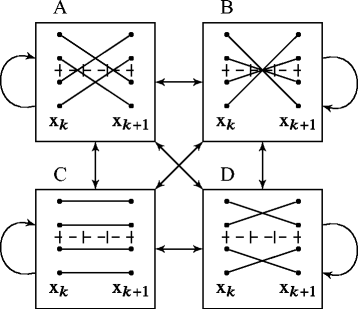
State machine for unconstrained 4-ASK symbol transitions
-
xk+1 can be reconstructed based on the current M+1 ADC output samples in case x k is known at the receiver, or x k can be reconstructed in case xk+1 is known (“forward”)
-
Possible ambiguity with transitions in state D (“ambiguity1”)
-
Possible ambiguity with transitions in state C (“ambiguity2”).

4.2 A state machine representation for reconstructible ASK sequences
In Section 4.1, it has been shown that only a subset of all possible transmit sequences can be distinguished based on the current ADC output pattern, when the transmit symbols x k are i.i.d.. The problem arises from the fact that the transitions contained in state D cannot be distinguished from the transitions contained in state C or vice versa. In the following, we describe how to avoid this problem by a systematic sequence construction. For this purpose, we model the transmit sequences by a state machine. The state machine is designed such that each possible realization of state transition sequences corresponds to a different output pattern at the receiver, i.e., each realization of the machine corresponds to a reconstructible sequence. We assume that the structure of the state machine is shared with the receiver. A segment of a reconstructible sequence is initiated and terminated with state A. This is due to the fact that with state A, x k and xk+1 are known, which is employed as starting point for backtracking. Moreover, the introduction of an additional constraint allows to some extent the utilization of both ambiguity states for sequence construction. First, one of the ambiguity states, e.g., state C, can be termed as a primary ambiguity state. The primary ambiguity can be considered for sequence construction nearly unconstrained. The residual, state D, is the secondary ambiguity which involves a constraint, e.g., such that after state D is visited only state B or state A is allowed, which retains the sequences segment unique for reconstruction. The corresponding state machine is illustrated in Fig. 3, where the B state subsequent to state D is termed B*. The adjacency matrix, describing the directed connections of the states, is given by

State machine for reconstructible 4-ASK sequences, with dependency on the whole prior sequence, \(P\left (x_{k} \vert x^{k-1}\right)\)
where the first three rows account for the outgoing connections for states A, B, and C, and the last two rows account for the outgoing connections from the states D and B*. The columns represent the incoming states in the order A, B, C, D, and B*. According to [31], the maximum entropy rate of sequences generated by this state machine can be computed with
where λmax is the largest real-valued eigenvalue of Aadj, and \(\boldsymbol {A}_{\text {adj}}^{n}\) describes Aadj raised to the power of n. Furthermore, according to [31] the transition probabilities that maximize the source entropy are computed with
where b j and b i are the ith and jth entry of the right hand eigenvector belonging to the eigenvalue λmax, respectively. The proposed state machine models sequences with infinite memory in terms of channel input symbols when expressing them by the Markov source introduced in Section 2 with a state corresponding to \(\mathrm {s}_{k}=\mathrm {x}_{k-L_{\text {src}}+1}^{k}\). To generate finite memory transmit sequences, a minor modification of the presented state machine is required, which is described in Appendix B. This modification leads, depending on the source memory Lsrc, to a slight reduction of the source entropy rate. However, according to Table 1, we already closely approach the maximum entropy of the state machine with infinite memory given in (20) by considering a memory of Lsrc=4.
5 Runlength-limited sequences
An alternative approach to model transmit sequences which can be uniquely reconstructed at a receiver with a 1-bit ADC is to use runlength-limited (RLL) sequences [32] in combination with FTN signaling. RLL sequences are a natural choice because they convey the information in the distances of zero-crossings or runlengths. As the temporal positions of a change of the signal should be controlled on a more fine-grained time-grid than Ts, we have to choose MTx>1 in (1), which corresponds to FTN signaling.
RLL sequences can be obtained from the so-called \(\left (d,k\right)\)-sequences, where d and k are the parameters which constrain binary sequences. In a \(\left (d,k\right)\)-sequence a 1 is followed by at least d and at most k 0s. The k property is introduced for practical purpose such as clock recovery which is neglected in this work, i.e., we assume \(k=\infty \). The corresponding state machine for a d-constrained sequence is illustrated in Fig. 4. The \(\left (d,k\right)\) sequence is subsequently transformed into a runlength-limited sequence by non-return-to-zero inverted (NRZI) encoding. An example is given as follows
where d=1. According to [31], the maximum entropy rate of such a sequence, which limits the corresponding achievable rate, depends on the adjacency matrix Aadj of the state machine and can be calculated by (19). The adjacency matrix describing the state machine in Fig. 4 is given by

State machine describing d-constrained sequences
where the rows correspond to the current states and the columns correspond to the following state. Furthermore, the transition probabilities for the source with maximum entropy are computed with (21). With this, the maximum achievable rates per symbol are given in Table 2.
The d constraint implies redundancy within the channel input sequence. However, in combination with a higher signaling rate, the RLL sequences can yield a benefit in terms of spectral efficiency for the case of 1-bit quantization at the receiver, which is different from the unquantized FTN [33]. This is due to the fact that the FTN-caused intersymbol interference cannot be corrected by the trellis-based receivers because of the loss of the additional amplitude information due to the 1-bit ADC. In this regard, the sequences need to be well shaped, such that the intersymbol interference does not induce a flip of the sign of current symbols. In this regard, the RLL sequences can tolerate some intersymbol interference, e.g., of the considered channel, at a relatively low cost in redundancy. In addition, the RLL sequences yield a higher concentration of the signal power of the transmit symbol sequence at lower frequencies. Depending on the bandwidth criterion, this might further increase the spectral efficiency. For complex transmit symbol sequences, we consider independent RLL sequences for the real and the imaginary part.
6 Maximization of a lower bound on the achievable rate using an expectation-based Blahut-Arimoto algorithm
In this section, we study a numerical input sequence optimization approach with respect to the achievable rate. In this regard, we discuss a strategy to optimize the transition probabilities of a given Markov source which models the channel input sequences. The set of transmit symbols \(\mathcal {X}\) is given and fixed. The objective of the optimization is an auxiliary channel based lower bound on the achievable rate similar to the one introduced in Section 3. The proposed sequence optimization approach [34] follows the principle of the iterative Markov source optimization suggested in [22]. Rewriting the information rate with the chain rule yields
where we use \(\mathrm {s}_{k}=\mathrm {x}_{k-L-N+1}^{k}\) on the RHS and with
The inequality in (24) holds as conditioning can only decrease entropy and the inequality in (25) holds according to the auxiliary channel lower bound, see Appendix C. The second term on the RHS of (25) can be expressed as
where the RHS can be practically evaluated with very long sequences. Considering a very long sequence, the argument of the limit on the RHS of (26) can be rewritten with the symbol transition probabilities Pi,j and the stationary distributionFootnote 7 μ i as
where \(\overline {(\cdot)}\) denotes the average over the specific state or state transition based on the number of their occurrences in the very long sequence realization. The second sum on the RHS of (27) can be also written as \(\sum _{i,j} \mu _{i} P_{i,j}\overline {(\cdot)}\), such that (27) can be rewritten as \( \sum _{i,j} \mu _{i} P_{i,j} \hat {T}_{i,j}\) with the coefficients
where the denominators account for the number of specific state transitions and states, respectively, occurring in the sequence xn. The quantities \(W\left (s_{k}, s_{k-1} \vert \boldsymbol {y}^{n} \right)\) and \(W\left (s_{k-1} \vert \boldsymbol {y}^{n} \right)\) are computed with the BCJR algorithm [30]. Based on the \(\hat {T}_{i,j}\) notation, the lower bound on the achievable rate in (25) is rewritten as
In the following, it is described how to chose Pi,j for maximizing the RHS of (29). In this regard, the so-called noisy adjacency matrix is given by
With (30), the transition probabilities which maximize the achievable rate are given by
where λmax is the largest real eigenvalue of \(\tilde {\boldsymbol {A}}_{\text {adj}}\) and b i and b j are entries of the corresponding eigenvector. The method is applied iteratively as \(\hat {T}_{i,j}\) itself is a function of Pi,j, where each iteration involves the generation of xn and yn.
Note that this optimization procedure does not take into account the power spectral density (PSD) of the resulting channel input signal. Moreover, the optimization has an influence on the average transmit power and, thus, on the SNR.
7 Numerical results
In this section, we numerically evaluate the achievable rate based on the lower bound in (10). The simulation-based computation of the RHS of (10), i.e., of the argument of the limit, is carried out based on a sequence of length n=106 symbols. Whenever the proposed sequence optimizaton strategy is applied, 19 iterations of the loop in the algorithm described in Section 6 have been carried out. The power containment bandwidth and the SNR are post-computed as the transmit signal bandwidth depends on the individual Markov source.
The correlation of the sequence of input symbols xn depends on the used Markov source and determines the power spectral density of the transmit signal. The coefficients of the discrete-time auto-correlation function of the transmit symbol sequence xn are given by
with the stationary input state distribution μ i . Hence, the corresponding PSD is given by the Fourier transform \( S_{\mathrm {x}}(f)= \frac {M_{\text {Tx}}}{T_{\mathrm {s}}} \sum _{k=-\infty }^{\infty } c_{k} e^{j 2 \pi \frac {k T_{\mathrm {s}} }{ M_{\text {Tx}} }f} \), where the infinite sum can be approximated by considering a very large number of coefficients. Together with the transfer function H(f) of the transmit filter h(t), the PSD of the transmit signal is given by \(S(f)=S_{\mathrm {x}}(f) \left |H(f)\right |^{2} \). In the following, we will refer to the two-sided power containment bandwidth B90% (or B95%), which implies that a certain amount, e.g., 10% (or 5%), of the transmit power is emitted outside the nominal bandwidthFootnote 8.
The power containment bandwidth, e.g., B90%, is used for computing the spectral efficiency as
where Ibpcu is the achievable rate w.r.t. one symbol symbol duration \(\frac {T_{\mathrm {s}}}{M_{\text {Tx}}}\). For numerical evaluation, we define the oversampling factor w.r.t. the power containment bandwidth, e.g., B90%, as
Moreover, also the SNR depends on the power containment bandwidth, e.g., B90%, and is defined as
Note that the transmit power depends on the Markov source modeling the input sequence xn and the transmit filter h(t). In the sequel, if not otherwise stated, we assume the 90% power containment bandwidth (B90%).
For different simulations, we use auxiliary channels with different memory N, cf. (9), as the computational complexity scales with the number of states s k which itself increases exponentially with N.Footnote 9 For computationally extensive cases, e.g., when the length of the channel impulse response L+1 is large because of a high signaling rate as is for MTx=3 or when the input symbol alphabet is large as is for MQAM=256, it is essential to consider an auxiliary channel law with a small N, e.g., N=0, to retain the computability. For the considered scenarios, we have observed that the achievable rate practically approaches its maximum when considering an auxiliary channel law with N≥ξ=MTx. Considering N=ξ=MTx implies that the condition in the channel law corresponds to the exact channel outputs \(\mathbf {y}^{k-1}_{k-N}\), whose time instances match to the noise samples \(\mathbf {n}^{k-1}_{k-\xi }\) which influence the current output y k , cf. (4). Moreover, from our experience, e.g., from [20], the impact on the lower bound of the achievable rate, e.g., when choosing N<ξ, is marginal at medium SNR and vanishes with increasing SNR, which is reasonable because the channel memory on the channel output arises from the noise process. An overview on the considered scenarios with 1-bit quantization at the receiver is given in Table 3.
To evaluate the burden for the use of 1-bit quantization and oversampling, we compare our approach with the channel without output quantization and RRC filtering with a roll-off factor of 0.3. In terms of FTN signaling, we compare with a reference system without quantization and with a roll-off factor equal to 1 and with various compression factors τT, cf. the notation in [33]. Moreover, we compare our results on the spectral efficiency with the AWGN channel capacity, normalized with the power containment bandwidth, assuming a flat spectrum.
7.1 Transmit pulse
Before considering the sequence design, the impact of the transmit pulse shape h(t) is examined in this section. The complexity of the trellis-based receiver scales exponentially with the length of the memory of the channel. In this context, transmit pulses with short duration in time domain are favorable and considered in this work explicitly. Standard transmit pulses are considered, such as the cosine pulse described by
Another widely used transmit pulse is the Gaussian pulse described by
where \(\alpha _{h}=\frac {1}{B_{3\text {dB}} T_{\mathrm {s}}} \sqrt {\frac {\log {2}}{2} }\) and B3dBTs=0.34. As the transmit pulse h(t), the Gaussian pulse with unit energy normalization is considered which is given by \(h_{\text {Gauss}}(t) = \left (\int _{-\infty }^{\infty } p_{\text {Gauss}}^{2}(t) dt \right)^{-\frac {1}{2}} p_{\text {Gauss}}(t)\). As a reference, also the rectangular pulse shape given by
is considered. The achievable rate for 16-QAM modulation with independent and uniformly distributed (i.u.d.) transmit symbols is illustrated in Fig. 5Footnote 10. Taking into account the power spectral density shown in Fig. 6, the spectral efficiency can be computed. The spectral efficiency w.r.t. B90% and w.r.t. B95% are shown in Figs. 7 and 8, respectively. In terms of spectral efficiency the Gaussian pulse and the cosine pulse show a comparable performance. Because the cosine pulse has a shorter duration in time domain, it is considered in the sequel.

Power spectral density for different transmit pulses

The spectral efficiency w.r.t. B90% for different transmit pulses

The spectral efficiency w.r.t. B95% for different transmit pulses
7.2 QAM
Based on the lower bound on the achievable rate in (10), Fig. 9 shows that the use of a higher order transmit symbol alphabet, namely 16-QAM, is beneficial. While with 1-bit quantization and without oversampling just 2 bits per channel use can be achieved (1 bit in the real and 1 bit in the imaginary component), with an increasing oversampling factor M the achievable rate increases. Moreover, it is illustrated that a sophisticated sequence design can further improve the achievable rate significantly compared to i.u.d. input symbols. In this regard, it is shown that the proposed method to model reconstructible sequences (Section 4), which is described for M=3, achieves an achievable rate fairly close to the optimized sequences (Section 6). With the approach based on reconstructible sequences, the achievable rate approaches the input entropy rate of 2·1.7678[bpcu], cf. Table 1, in the high SNR regime, where the factor 2 is due to the use of a complex modulation. The corresponding PSDs are shown in Fig. 10. Note that the sequence optimization depends on the SNR and that the illustrated spectra consider high SNR (30 dB). Figure 11 shows that the achievable rate can be further increased by utilizing even larger modulation alphabets, e.g., 64-QAM or 256-QAM. In this regard, note that the achievable rate for a 256-QAM alphabet is larger than \(2 \log _{2} (M+1)\), for M=2 and M=3.Footnote 11 This is remarkable, because it is higher than the upper limit for the noiseless channel without receive filter described in Appendix D. We explain this by the circumstance that with the receive filter the system impulse response is enlarged, such that new signal evolutions are enabled, leading to more zero-crossing patterns. This is in line with the data processing lemma because the subsequent quantization is a suboptimal processing step. Moreover, it is also remarkable, because \(2 \log _{2} (M+1)\) is the maximum achievable rate for flash ADC based sampling with M comparators. For 64-QAM and 256-QAM, the achievable rate is lower-bounded by the utilization of a simplifying auxiliary channel model with N=0. The sequence optimization only considers a peak power constraint and no bandwidth constraint. Because of this and the circumstance that our SNR definition involves the bandwidth, we expect that at low SNR the actual capacity is higher than that computed with our approach.
The spectral efficiency as defined in (33) is shown in Fig. 12. It can be observed that the spectral efficiency of i.u.d. input sequences might be higher than with optimized input sequences (Section 6) or with reconstructible sequences designed according to the approach presented in Section 4. This effect happens as we do not consider any spectral shaping during the sequence design approaches besides the choice of the pulse shape. In this regard, the bandwidth depends on the sequence design and the spectral efficiency can decrease. However, as the oversampling factor inversely scales with the bandwidth, the sequence design is still superior in comparison to sequences of i.u.d. symbols, as we will point out in detail in Section 7.5.

Spectral efficiency (B90%) versus SNR considering QAM transmit symbols
7.3 PSK
Figure 13 shows the lower bound on the achievable rate in (10) for PSK symbol alphabets and 1-bit quantization and oversampling at the receiver. The PSK input alphabet deserves special attention because the corresponding transmit signal has a relatively low peak to average power ratio, which is favorable in terms of linearity requirements of the transmit power amplifier. The case of 8-PSK modulation is remarkable, because at high SNR, the maximum input entropy of 3 bpcu is almost achievable with M=3.

Achievable rate versus SNR considering PSK transmit symbols
Unlike as for QAM, due to the constant modulus transmit symbols, the average transmit power is not strongly influenced by the applied sequence optimization strategy. However, as discussed for QAM modulation, the nominal bandwidth depends on the PSD of the transmit signal and, thus, on the applied Markov source which describes the transmit symbol sequences. Thus, the SNR in (35) depends on the chosen sequence design, which explains the slight horizontal shift of corresponding markers in Fig. 13.
The corresponding spectral efficiency (B90%) is shown in Fig. 14. In some exceptional cases i.u.d. channel input symbols yield a higher spectral efficiency in comparison to the optimized sequences design. As explained in Section 7.2, in these cases sequence optimization (Section 6) yields an increased bandwidth implying a reduced effective oversampling factor Moversampling. The relation between the effective oversampling factor and the spectral efficiency is evaluated later in Section 7.5. Comparing 16-PSK and 16-QAM in terms of the spectral efficiency, it can be observed that 16-QAM is superior for M=2 and M=3.

Spectral efficiency (B90%) versus SNR considering PSK transmit symbols
7.4 Faster-than-Nyquist signaling
In the following, we evaluate the achievable rate with FTN signaling, i.e., MTx>1, on the one hand for RLL sequences as discussed in Section 5 and on the other hand also for transmit sequences with i.u.d. symbols and for optimized sequences (Section 6) with QPSK and 16-QAM input alphabets. Here, we choose an equal signaling and sampling rate, i.e., M=1.
Regarding the auxiliary channel law utilized for lower-bounding the achievable rate, the maximum can be practically approached by considering N=ξ=MTx. However, we have considered memories of N=1 or N=0, not necessarily N=MTx, to limit the computational complexity.
In Fig. 15, based on (10), lower bounds on the achievable rate per channel use are shown, where a channel use corresponds to a transmit symbol duration \(\frac {T_{\mathrm {s}}}{M_{\text {Tx}}}\). In general, it can be observed that the achievable rate decreases with an increasing compression factor MTx. This behavior is a consequence of the fact that the duration of one channel use is scaled down with MTx. In this regard, the benefit of FTN is not reflected in Fig. 15. However, Fig. 15 allows a comparison of the achievable rate with different sequence design approaches for an equal MTx.

Achievable rate with FTN signaling, M=1, a channel use corresponds to time interval \(\frac {T_{\mathrm {s}}}{M_{\text {Tx}}}\)
Figure 15 confirms that the maximum achievable rate for RLL sequences, cf. Table 2, can be achieved. For a RLL sequence with d=1 and MTx=3, we have observed that the achievable rate does not approach the source entropy rate when using the receive filter in (2) (not shown in Fig. 15). For this special case, we choose a receive filter with a shorter impulse response
which corresponds to a larger receive bandwidth. In the figures, we refer to this exception by the notation wideband Rx. In this case, the achievable rate converges to the source entropy rate. However, due to the larger bandwidth of the receive filter, more noise is captured such that the achievable rate saturates at higher SNR.
Moreover, it can be observed that the optimized sequences (Section 6) yield a slightly larger achievable rate than RLL sequences. Compared to the RLL sequences, the sequence optimization strategy has more degrees of freedom for the construction of zero-crossings. Surprisingly, MTx=3 yields an even larger achievable rate in the high SNR as compared to MTx=2, which is counter intuitive. On one hand, increasing the signaling rate implies a relative expansion of the system impulse response w.r.t. \(\frac {T_{\mathrm {s}}}{M_{\text {Tx}}}\) which in our case strongly attenuates fast signal transitions. This is why at low SNR, MTx=2 holds a benefit in the achievable rate w.r.t. to a channel use in comparison to MTx=3. At high SNR, utilization of MTx=3 can effectively exploit more bandwidth for communication. This is possible due to the fact that the considered transmit pulse is not strictly bandlimited. Finally, the expansion of the system impulse response provides more degrees of freedom which is in general favorable for the construction of zero-crossings.
In addition, a 16-QAM alphabet has been considered for sequence optimization (Section 6) with MTx=2. Due to the additional degrees of freedom, this approach shows a much better performance in terms of achievable rate compared to the other waveforms with MTx=2.
We have compared our results with RRC-matched filtering-based FTN signaling without quantization. The compression in time is such that the transmit pulses have a distance of τT·T x , where T x would be the conventional transmit symbol duration without FTN. We have computed a lower bound on the achievable rate by using a truncation-based auxiliary channel law where we have used for τT=0.5, 0.4, and 0.3 a truncated system impulse response of length (L+1)=3, 5, and 6, respectively.
The PSDs of the different sequence designs are shown in Fig. 16. The consideration of runlength-limited sequences implies that the signal energy is concentrated at lower frequencies. To show the benefits of FTN signaling, we evaluate its performance in terms of the spectral efficiency (B90%) in Fig. 17. This presentation also enables a fair comparison for different compression factors MTx, as the achievable rate is normalized with respect to the 90% power containment bandwidth. In Fig. 17, it can be observed that with increasing MTx and, hence, also equally increasing sampling rate, the spectral efficiency significantly increases for all approaches for the transmit symbol sequence generation. Moreover, Fig. 17 shows that for a given MTx, RLL sequences show a superior performance in comparison to the other approaches in terms of spectral efficiency. This holds even in comparison to the case where the large 16-QAM modulation alphabet is used. The additionally required transmit power in comparison to the unquantized FTN is less than 4 dB when operating at an SNR below 15 dB.

Power spectral density for different FTN sequence designs

Spectral efficiency (B90%) versus SNR, with FTN signaling, M=1
Moreover, by the comparison of Figs. 17 and 12, we make the important observation that the communication based on the FTN signaling scheme requires a significantly lower SNR. This can be explained by the fact that the transmit filter h(t) in (36) is not strictly bandlimited. In this regard, the spectral copies at a signaling rate of \(\frac {1}{T_{s}}\) when MTx=1 implicitly restrict the sequence design which cannot be compensated by a large input alphabet. The faster signaling rate offers more degrees of freedom for the sequence design at higher frequencies. However, in a scenario with strict bandlimitation [23], e.g., by considering Nyquist pulses, this effect vanishes.
7.5 Relation of the spectral efficiency and the oversampling factor in the high SNR limit
Figure 18 illustrates the spectral efficiency (B90%) in the high SNR limit as a function of the effective oversampling factor (34). Alternatively, the 95% power containment bandwidth is considered in Fig. 19. Note that spectral efficiency and also the oversampling factor inversely scale with the bandwidth. The results confirm the intuitive presumption that in case of 1-bit channel output quantization an increase of the sampling rate can yield an increase in spectral efficiency. The illustration shows a fair comparison between the presented approaches because the considered effective oversampling factor takes into account the bandwidth of the transmit signal. The results are compared with the results known from the literature, which have been adapted w.r.t. the power containment bandwidth. We also compare our results with the result on the achievable rate over a bandlimited noiseless channel with 1-bit output quantization in [3], which we could not normalize with the power containment bandwidth as the considered Zakai processes do not have Fourier transformations. Unlike the existing literature on communication over noisy channels with 1-bit quantization at the receiver [5–7] which indicates only moderate benefits from oversampling, the proposed communication schemes show a clear advantage of oversampling in terms of the spectral efficiency. The results are also comparable with the recent results which are based on strictly bandlimited channels with RRC filtering [23]. Moreover, the proposed methods are compared to the maximum achievable rate for systems with a standard flash ADC with Nyquist rate sampling at the receiver with the same number of comparator operations per time interval. For a strictly bandlimited channel, its achievable rate is given by \(2 \log _{2}\left (M_{\text {oversampling}} +1 \right)\), which we normalize w.r.t. the power containment bandwidth based on a frequency flat spectrum. Some of the approaches given in the present work are comparable and even superior in terms of achievable rate in comparison to the flash ADC approach and the analytical results on the noiseless channel given in [3]. Note that pipelined ADCs require less comparators in comparison to the flash ADCs. However, because of the additional inter-stage processing in pipelined ADCs, a comparison is not straightforward.

Spectral efficiency (B90%) versus effective oversampling factor (B90%) in the high SNR limit; for FTN (MTx>1), it holds that M=1

Spectral efficiency (B95%) versus effective oversampling factor (B95%) in the high SNR limit; for FTN (MTx>1), it holds that M=1
8 Conclusions
We have studied the achievable rate for an additive Gaussian noise channel with 1-bit output quantization and oversampling at the receiver, which is promising in terms of a simplification of circuitry and a reduction of the energy consumption at the receiver. As the transmit signal is not strictly bandlimited, we have considered power containment bandwidth criteria with 90% and alternatively 95% power containment. The transmit sequences are constructed based on various QAM and PSK input symbol alphabets and various signaling rates. Concrete sequence designs, namely reconstructible 4-ASK (and with this 16-QAM) sequences and runlength-limited sequences for faster-than-Nyquist signaling rates, are proposed. Furthermore, a sequence optimization strategy is studied which approaches the Markov capacity in the high SNR regime. The performance is evaluated in terms of the achievable rate and the spectral efficiency. We have observed that the proposed approaches outperform the existing methods on communication with 1-bit quantization and oversampling at the receiver. For a number of methods, it has been shown that 1-bit quantization and oversampling at the receiver yields a comparable or even superior spectral efficiency than conventional amplitude quantization using a flash converter with the same number of comparator operations per time interval.
One key observation is that among the proposed methods, the spectral efficiency is maximized by FTN signaling. This suggests that for the channel input signal, the resolution in time is preferable in comparison to the resolution in amplitude. However, it is known for the unquantized case that FTN exploits the excess bandwidth [33], such that it can be expected that the advantage of FTN vanishes for more strict spectral constraints, cf. [23]. In summary, the results show that the use of receivers with oversampled 1-bit quantization is promising. The proposed ideas are a first step to a more complete understanding of the achievable rate and of an optimal transmit sequence design for such channels. Aspects like the robustness of these signaling schemes towards jitter and timing synchronization errors remain for further study. It is shown that the presented methods based on 1-bit quantization and oversampling at the receiver require only 2−3 dB more transmit energy (at 5−10 dB SNR and 90% power containment bandwidth) in comparison to a conventional communication system design with Nyquist sampling and high resolution in amplitude.
9 Appendix A
9.1 The system impulse response for reconstructible sequences
We consider a symmetric system impulse response ranging over 3Ts. With the parameters M=3 and MTx=1, the discrete system impulse response can be described by nine coefficients, by \(\boldsymbol {v}=\left [ v_{4},\ldots,v_{0},\ldots,v_{4}\right ]^{T}\). The output patterns displayed in the different states in Fig. 2 are functions of two consecutive channel input symbols x k and xk+1 taken from a 4-ASK constellation, e.g., \(\mathrm {x}_{k} \in \left \{-3,-1,1,3 \right \}\). Because of the length of the system inpulse response, the neighboring channel input symbols xk−1 and xk+2 are also considered. For the interference from xk−1 and xk+2, we assume a maximum amplitude and distinguish between positive and negative sign. For each transition type A …D, inequalities can be formulated which describe the signal shape according to the desired pattern at the output of the ADC (assuming no noise). Exploiting the symmetry of the impulse response v, its coefficients have to fulfill the following inequalities to be able to apply the state representation in Fig. 3: \(\boldsymbol {B}^{T}_{\textrm {constr.\ i}} \left [ v_{0}, \ldots,v_{4} \right ]^{T} > \boldsymbol {0} \textrm {, for}\ i=\{\mathrm {A},\ldots,\mathrm {D}\}\), where 0 denotes a column vector containing 8 zeros and where the Bconstr. i express the state transition specific constraints and are given by
which describe the combinations of the input symbols. Note that some of the constraints are redundant. Moreover, symmetries have been exploited. Besides the illustrated triangular waveform with \(\left [ v_{0},\ldots,v_{4} \right ]=\left [1, 0.666, 0.333, 0, 0 \right ]\), the waveform with the transmit pulse given in (36) jointly with the assumptions on the receive filter in Section 2 corresponding to the coefficients \(\left [ v_{0},\ldots,v_{4} \right ]=\left [0.9449, 0.759, 0.387, 0.1037, 0.0042 \right ]\) fulfills these constraints.

State machine to generate reconstructible 4-ASK sequences with finite memory
10 Appendix B
10.1 Reconstructable 4-ASK sequences with finite memory
The system model introduced in Section 2 relies on channel input sequences defined by a Markov process where the states correspond to \(\mathrm {s}_{k}=\mathrm {x}^{k}_{k-L_{\text {scr}}+1}\), i.e., the source has finite memory. Differently, in the state machine in Fig. 3, a channel input symbol depends on an infinite number of previous channel input symbols. Thus, we will modify the state machine such that an output symbol just depends on a finite number of Lscr past output symbols. For this purpose, we exclude the state transition from B* to B* in the state machine in Fig. 3. The loss in terms of the source entropy rate can be compensated by introducing further states like B**, B***, etc. This implies that the process returns to state A after passing state D with a maximum number of transitions which can be easily translated into the state representation used for Markov sources in this work. The dashed boxes in Fig. 20 show the state machines for reconstructible sequences for \(L_{\text {scr}}=1, \dots,4\). The corresponding adjacency matrices are given by
11 Appendix C
11.1 A lower bound based on the auxiliary channel law (reverse)
The auxiliary channel lower bound in [29] used in (10) is introduced as
where W(·) is the auxiliary channel law (9). We will show with similar steps as used in [29] that its reverse formulation also applies, also for a conditional mutual information. The RHS of (25) can be written as \({\lim }_{n \to \infty } \frac {1}{n} \sum _{k=1}^{n} \underline {I}_{W}(\mathrm {s}_{k};\mathbf {y}^{n} \vert \mathrm {s}_{k-1})\), and its terms are given by
To show that \(\underline {I}_{W}\left (\mathrm {s}_{k};\mathbf {y}^{n} \vert \mathrm {s}_{k-1}\right)\) lower-bounds \({I}\!\left (\mathrm {s}_{k};\mathbf {y}^{n} \vert \mathrm {s}_{k-1}\right)\), we consider the difference given by
where D(·∥·) is the Kullback-Leibler divergence [35] which is always non-negative [36, Th. 8.6.1].
12 Appendix D
12.1 Upper-bounding the capacity of the noiseless channel without receive filter
We consider a special case with the transmit pulse h(t)=hcos(t), a receive filter with g(t)=δ(t) and n(t)=0, such that the input signal of the ADC is x(t), which is a weighted sum of time shifted transmit pulses h(t). We consider a conventional signaling rate with MTx=1 such that the transmit signal is denoted by
With this, the signal in a time interval of two consecutive symbols xk−1 and x k is given by
which describes a raised or lowered cosine function in the interval with the running time variable τ. Its frequency is such that x(t) has at max one zero-crossing per time interval kTs≤τ<(k+1)Ts. Now, we consider that this signal is quantized with 1-bit and sampling rate \(\frac {M}{T_{\mathrm {s}}}\). The fact that there is at most one zero-crossing in the time interval Ts implies that the maximum output entropy and with this also the capacity are upper-bounded by \(2\log _{2}(M+1)\), where the factor 2 accounts for the complex equivalent.
Notes
A matched filter would also depend on the sequence design, i.e., on the statistical dependencies of the individual x k .
Thus, the input symbols are not placed on the real and imaginary axes which are the thresholds of the applied 1-bit quantizer.
The system impulse response v(t) is normalized implicitly, because it is considered that h(t) has unit energy normalization.
The considered integrate-and-dump receiver is an exceptional case, where the noise correlation can be perfectly described on the sampling grid (D=1), although there is no bandlimitation.
For the computation, symmetries in the input sequences can be exploited to reduce the number of integrations.
The case of QAM sequences follows by using the concept for the real as well as for the imaginary axis.
The stationary distribution μ i can be computed based on Pi,j.
In case of asymmetric spectra, it is considered that the power of the out-of-band radiation is equally splitted into the frequency range towards \(f=\infty \) and the frequency range towards \(f= -\infty \).
This is true as long as L+N>Lsrc holds, cf. the state definition in Sec. 3.1.
Note that the SNR definition contains the bandwidth, which then yields a relatively low SNR for scenarios with hrect(t).
Fig. 5 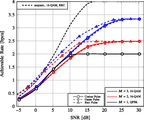
The achievable rate for different transmit pulses
We expect that for M>3 a larger input alphabet is required to obtain an achievable rate larger than \(2 \log _{2} (M+1)\).
Fig. 9 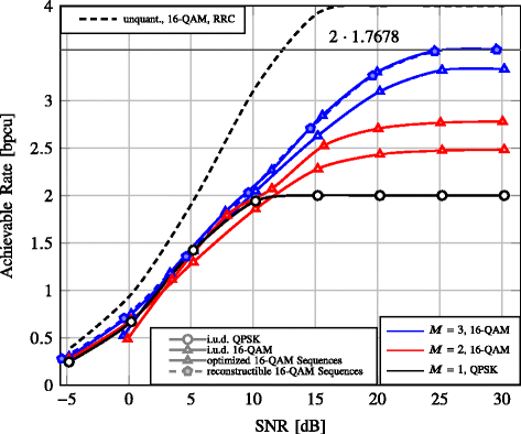
Achievable rate with 1-bit quantization and M-fold oversampling, QAM modulation, and various sequence designs, N=1
Fig. 10 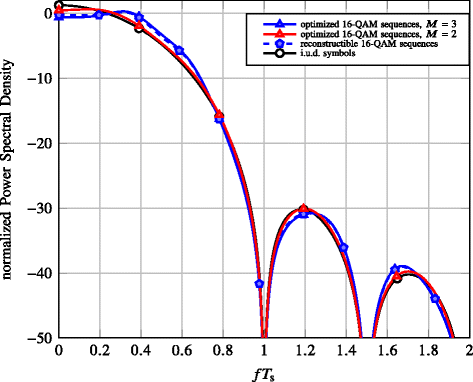
Power spectral density for different sequence designs based on cosine transmit pulses
Fig. 11 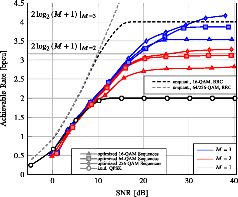
Achievable rate for different oversampling rates and QAM modulation orders; for comparison, upper bound on the achievable rate when using M comparators in a flash ADC with the same number of comparator operations per time interval (horizontal lines)


References
J Singh, O Dabeer, U Madhow, On the limits of communication with low-precision analog-to-digital conversion at the receiver. IEEE Trans. Commun.57(12), 3629–3639 (2009).
EN Gilbert, Increased information rate by oversampling. IEEE Trans. Inf. Theory. 39(6), 1973–1976 (1993).
S Shamai (Shitz), Information rates by oversampling the sign of a bandlimited process. IEEE Trans. Inf. Theory. 40(4), 1230–1236 (1994).
T Koch, A Lapidoth, in Proc. of the IEEE Convention of Electrical and Electronics Engineers in Israel. Increased capacity per unit-cost by oversampling (Eilat, 2010).
W Zhang, A general framework for transmission with transceiver distortion and some applications. IEEE Trans. Commun.60(2), 384–399 (2012).
S Krone, GP Fettweis, in Proc. of the IEEE Sarnoff Symp. Capacity of communications channels with 1-bit quantization and oversampling at the receiver (Newark, 2012).
S Krone, GP Fettweis, in Proc. of the IEEE International Symposium on Personal, Indoor, and Mobile Radio Communications. Communications with 1-bit quantization and oversampling at the receiver: benefiting from inter-symbol-interference (Sydney, 2012).
JE Mazo, Faster-than-Nyquist signaling. Bell Syst. Tech. J.54(1), 1451–1462 (1975).
JB Anderson, F Rusek, V Öwall, Faster-than-Nyquist signaling. Proc. IEEE. 101(8), 1817–1830 (2013).
T Hälsig, L Landau, GP Fettweis, in Proc. of the IEEE Vehicular Technology Conference (Spring). Information rates for faster-than-Nyquist signaling with 1-bit quantization and oversampling at the receiver (Seoul, 2014).
L Landau, S Krone, GP Fettweis, in Proc. of the International ITG Conference on Systems, Communications and Coding. Intersymbol-interference design for maximum information rates with 1-bit quantization and oversampling at the receiver (Munich, 2013).
A Mezghani, JA Nossek, in Proc. IEEE Int. Symp. Inform. Theory (ISIT). On ultra-wideband MIMO systems with 1-bit quantized outputs: performance analysis and input optimization (Nice, 2007), pp. 1286–1289.
A Mezghani, JA Nossek, in Proc. IEEE Int. Symp. Inform. Theory (ISIT). Capacity lower bound of MIMO channels with output quantization and correlated noise (Cambridge, 2012), pp. 1732–1736.
J Mo, RW Heath Jr, Capacity analysis of one-bit quantized MIMO systems with transmitter channel state information. IEEE Trans. Sign. Process.63(20), 5498–5512 (2015).
A Gokceoglu, E Björnson, EG Larsson, M Valkama, in Proc. IEEE Int. Conf. Commun. (ICC). Waveform design for massive MISO downlink with energy-efficient receivers adopting 1-bit ADCs (Kuala Lumpur, 2016), pp. 1–7.
A Gokceoglu, E Björnson, EG Larsson, M Valkama, Spatio-temporal waveform design for multi-user massive MIMO downlink with 1-bit receivers. IEEE J. Sel. Top. Signal Process. 11(2), 347–362 (2016).
J Singh, U Madhow, Phase-quantized block noncoherent communication. IEEE Trans. Commun.61(7), 2828–2839 (2013).
M Stein, S Theiler, JA Nossek, Overdemodulation for high-performance receivers with low-resolution ADC. IEEE Wirel. Commun. Lett.4(2), 169–172 (2015).
G Zeitler, AC Singer, G Kramer, Low-precision A/D conversion for maximum information rate in channels with memory. IEEE Trans. Commun.60(9), 2511–2521 (2012).
L Landau, GP Fettweis, in Proc. of the IEEE Int. Workshop on Signal Processing Advances in Wireless Communications. Information rates employing 1-bit quantization and oversampling (Toronto, 2014).
J Chen, PH Siegel, Markov processes asymptotically achieve the capacity of finite-state intersymbol interference channels. IEEE Trans. Inf. Theory. 54(3), 1295–1303 (2008).
A Kavcic, in Proc. IEEE Glob. Comm. Conf. (GLOBECOM). On the capacity of Markov sources over noisy channels. vol.5 (San Antonio, 2001), pp. 2997–3001.
L Landau, M Dörpinghaus, GP Fettweis, 1-Bit quantization and oversampling at the receiver: communication over bandlimited channels with noise. IEEE Commun. Lett.21(5), 1007–1010 (2017).
T Hälsig, L Landau, GP Fettweis, in Proc. of the IEEE Vehicular Technology Conference (Fall). Spectral efficient communications employing 1-bit quantization and oversampling at the receiver (Vancouver, 2014).
G Singh, L Landau, GP Fettweis, in Proc. of the International ITG Conference on Systems, Communications and Coding. Finite length reconstructible ask-sequences received with 1-bit quantization and oversampling (Hamburg, 2015).
HD Pfister, JB Soriaga, PH Siegel, in Proc. IEEE Glob. Comm. Conf. (GLOBECOM). On the achievable information rates of finite state ISI channels (San Antonio, 2001).
D Arnold, HA Loeliger, in Proc. IEEE Int. Conf. Commun. (ICC). On the information rate of binary-input channels with memory. vol. 9 (Helsinki, 2001), pp. 2692–26959.
Z Zhang, TM Duman, EM Kurtas, Information rates of binary-input intersymbol interference channels with signal-dependent media noise. IEEE Trans. Magn.39(1), 599–607 (2003).
DM Arnold, H-A Loeliger, PO Vontobel, A Kavcic, W Zeng, Simulation-based computation of information rates for channels with memory. IEEE Trans. Inf. Theory. 52(8), 3498–3508 (2006).
L Bahl, J Cocke, F Jelinek, J Raviv, Optimal decoding of linear codes for minimizing symbol error rate (corresp.)IEEE Trans. Inf. Theory. 20(2), 284–287 (1974).
CE Shannon, A mathematical theory of communications. Bell Syst. Tech. J.27:, 379–423 (1948).
KA Schouhamer Immink, Runlength-limited sequences. Proc. IEEE. 78(11), 1745–1759 (1990).
F Rusek, JB Anderson, Constrained capacities for faster-than-Nyquist signaling. IEEE Trans. Inf. Theory. 55(2), 764–775 (2009).
L Landau, M Dörpinghaus, GP Fettweis, in Proc. of the IEEE Int. Conf. on Ubiquitous Wireless Broadband. Communications employing 1-bit quantization and oversampling at the receiver: faster-than-Nyquist signaling and sequence design (Montreal, 2015).
S Kullback, RA Leibler, On information and sufficiency. Ann. Math. Statist.22(1), 79–86 (1951).
TM Cover, JA Thomas, Elements of Information Theory, 2nd edn. (Wiley-Interscience, Hoboken, 2006).
Acknowledgements
We thank the referees for very useful comments.
Funding
This work has been supported in part by the German Research Foundation (DFG) within the Collaborative Research Center SFB 912 “Highly Adaptive Energy-Efficient Computing.”
Availability of data and materials
Not applicable.
Author information
Authors and Affiliations
Contributions
All authors contributed to the conception and design of the study. LL drafted the manuscript and did the simulation work. All authors contributed to the interpretation of the results. MD reviewed and edited the manuscript and helped with the revisions. All authors read and approved the final manuscript.
Corresponding author
Ethics declarations
Competing interests
The authors declare that they have no competing interests.
Publisher’s Note
Springer Nature remains neutral with regard to jurisdictional claims in published maps and institutional affiliations.
Additional information
Parts of this paper have been published at SPAWC 2014, ICUWB 2014, and ICUWB 2015
Rights and permissions
Open Access This article is distributed under the terms of the Creative Commons Attribution 4.0 International License(http://creativecommons.org/licenses/by/4.0/), which permits unrestricted use, distribution, and reproduction in any medium, provided you give appropriate credit to the original author(s) and the source, provide a link to the Creative Commons license, and indicate if changes were made.
About this article

Cite this article
Landau, L.T.N., Dörpinghaus, M. & Fettweis, G.P. 1-bit quantization and oversampling at the receiver: Sequence-based communication. J Wireless Com Network 2018, 83 (2018). https://doi.org/10.1186/s13638-018-1071-z
Received:
Accepted:
Published:
DOI: https://doi.org/10.1186/s13638-018-1071-z