- Research
- Open access
- Published:
A new blind algorithm for channel estimation in OFDM-based amplify-and-forward two-way relay networks
EURASIP Journal on Wireless Communications and Networking volume 2018, Article number: 183 (2018)
Abstract
In this paper, we propose a blind channel estimation algorithm for the amplify-and-forward (AF) two-way relay network (TWRN) which consists of two terminal nodes and one relay node. The orthogonal frequency division multiplexing (OFDM) modulation is adopted for frequency selective channel. Both cyclic prefix (CP) and zero padding (ZP) are considered. The two cascaded channels are estimated in two steps. First, the cascaded channel causing the self-interference is estimated using a proposed power reduction method. Then, the other cascaded channel from source to destination is estimated by subspace method. Closed-form formulas for channel estimates are derived. In addition, we also carry out the theoretical mean square error analysis and derive the approximated Cramer-Rao bounds.
1 Introduction
Research on wireless relay networks became popular since the pioneering work [1] developed low-complexity cooperative diversity strategies. In [1], data streams flow unidirectionally from the source to the relay and then to the destination. This network structure is known as the one-way relay network (OWRN). However, since most communication systems are bidirectional, it is necessary to consider the situation when the source node and the destination node exchange their roles. Such a relay network is known as the two-way relay network (TWRN). In TWRN, the relay treats the received signals in a “network coding”-like manner [2], and the terminals can recover the signal collision since they know their own transmitted signals. As a result, the overall communication rate between two source terminals in TWRN is approximately twice that achieved in OWRN [3].
Despite its throughput advantage, TWRN faces more challenges in terms of transceiver design, relay processing optimization, and transmission protocol development. In [4], the capacity analysis and the achievable rate region for amplify-and-forward (AF) and decode-and-forward (DF) TWRN are explored. In [5], the authors point out that the throughput of AF-TWRN is 1.5 times of DF-TWRN. The distributed space-time code (STC) at relays for both AF-TWRN and DF-TWRN has been developed in [6]. Moreover, the optimal beamforming with full channel knowledge at the multi-antenna relay that maximizes the overall system capacity of AF-TWRN is derived in [7]. In [8], the authors address the problem of robust linear relay precoder and destination equalizer design for multiple-input multiple-output relay systems. In [9], the authors compare several network-coding AF-TWRN and consider imperfect time synchronization. Most existing works on TWRN [2–9] have assumed perfect channel state information (CSI) at the relay node and/or the source terminals. While traditional channel estimation methods can be applied to DF-TWRN, the channel estimation problem for AF-TWRN is more challenging due to the self-interfering signals.
In traditional channel estimation methods for point-to-point systems, they can be divided into two groups: data-aided (DA) [10–17] and non data-aided (blind) [18–26]. In general, DA channel estimation methods differ in the way they interpolate or filter punctual DA least square (DA-LS) channel estimates over data subcarriers. This can be accomplished using time-frequency Wiener filtering [10, 11], which is optimal in the minimum mean square error (MMSE) sense if knowledge of the channel statistics (KCS) is available. On the other hand, channel estimation can be accomplished by elaborating raw estimates in the time domain using a discrete Fourier transform (DFT)-based scheme. In [12], the MMSE channel estimator working in the time domain has been proposed. In order to reduce computational complexity, using the singular value decomposition and several low-rank approximations to the MMSE estimator has been proposed in [13] and [14]. Li et al. [12–14] also require complete KCS. In [15], the authors compare the MMSE approach with maximum likelihood (ML) channel estimation, where complete KCS is not required. This latter approach works well with dense multipath channels and quasi-uniform profiles. In practice, after the inverse DFT (IDFT), not all the channel impulse response (CIR) samples are significant because many may correspond to delays where no propagation channel paths are actually present. Therefore, the authors in [16] exploit this idea to estimate channel. In [17], the authors propose a method to approach the MMSE channel estimation performance, while avoiding the need for a priori KCS.
For blind channel estimation methods, earlier works require either higher order statistics (HOS) of the received data [18] or over-sampling at the receiver [19]. By exploiting linear redundant precoding, only second-order statistics (SOS) of the received data is required and these methods are robust to channel order overestimation [20, 21]. Another popular blind algorithm is the so-called subspace-based algorithm which was originally developed in [19]. The subspace method has simple structure and achieves good performance. In [22], a blind channel identification method by exploiting virtual carriers (VC) is derived. In [23], a generalization in cyclic prefix (CP) systems is proposed. By arranging the received data appropriately, [23] generates a rank-deduction matrix, and thus, subspace method can work. In [24], the authors propose another simpler arrangement of the received data. Pan and Phoong [25] and [26] utilize the repetition method to reduce the number of required received data and consider the existence of VCs.
As in the traditional point-to-point systems, study of channel estimation algorithm is also demanded for AF-TWRN systems [27–34]. DA channel estimation methods for AF-TWRN are proposed in [27–30]. Gao et al. [27] develops an optimal training design for flat-fading environment. The authors also combine their algorithm with orthogonal frequency division multiplexing (OFDM) to estimate the channel impulse responses for frequency selective environment in [28]. The case of multiple-input multiple-output is considered in [29], and [30] provides two channel training algorithms for channel estimation.
On the other hand, [31–34] are blind channel estimation methods. In [31], the authors propose a ML approach to estimate the flat-fading channels blindly, but the transmitted signals are limited to constant modulus modulation. Zhao et al. [32] find a closed-form solution and thus provides a low-complexity ML algorithm. For non-constant modulus modulation, [33] gives an iterative algorithm, which is based on the maximum a posteriori (MAP) approach, and it requires a large number of received blocks. In [34], the authors consider the frequency selective environment. They apply a non-unitary linear precoding at both terminals and derive a blind channel estimation algorithm from SOS of the received signals. However, the use of non-unitary linear precoding leads to degradation in bit error rate (BER) performance.
In this paper, we develop a blind channel estimation algorithm for AF-TWRN under OFDM modulation. Our method consists of two steps. The first step is to estimate the cascaded channel causing the self-interference. Since the terminal knows its own transmitted signal, we choose the method based on power reduction to estimate the channel, which is also named LS method. The self-interference signal can be removed by using the estimated channel. The second step is to estimate the cascaded channel from source to destination. We utilize the rank reduction method, which is also known as subspace-based algorithm [23–26]. This is because subspace methods do not require complete KCS, work well with all multipath channels, and achieve good performance. Closed-form formulas for these two cascaded channel estimates are derived. The theoretical performance analysis and approximated Cramer-Rao bounds (ACRB) are given as well. The proposed method can be applied to both CP-based and zero padding (ZP)-based OFDM systems. Simulation results will be provided to show the performance of the proposed method.
The rest of this paper is organized as follows. The system model for CP-OFDM AF-TWRN is introduced in Section 2. Section 3 describes the proposed algorithm for blind channel estimation. In Section 4, we analyze the performance of the proposed channel estimation methods and the ACRBs. Simulation results are presented in Section 5, and concluding remarks are made in Section 6. The results in Section 3.1 and 3.2 of this paper have appeared in a conference paper [35].
Notation In this paper, E{x} stands for the statistical expectation of the random variable x. The symbols AT, A∗, and A† denote the transpose, the complex conjugate, and the conjugate-transpose of matrix A, respectively. ∥A∥F is the Frobenius norm of matrix A. If A is a square, tr(A) denotes the trace of matrix A. Im is the m×m identity matrix, whereas 0 represents an all-zero matrix with appropriate dimension. \(\jmath =\sqrt {-1}\) is the imaginary unit. Tm(c) and \(\tilde {\mathbf {T}}_{m}(\mathbf {c})\) are two Toeplitz matrices respectively defined as
and
where c=[c1,c2,…,cn]T is an arbitrary vector.
2 System model
Consider a TWRN with two terminal nodes \(\mathbb {T}_{1}\) and \(\mathbb {T}_{2}\), and one relay node \(\mathbb {R}\), as shown in Fig. 1. Each node has one antenna which cannot transmit and receive simultaneously. The channel from \(\mathbb {T}_{i}\) to \(\mathbb {R}\) is denoted as \(\mathbf {f}_{i}=[f_{i,0}^{},f_{i,1}^{},\ldots,f_{i,L}^{}]^{T}\), whereas the one from \(\mathbb {R}\) back to \(\mathbb {T}_{i}\) is denoted as \(\mathbf {g}_{i}=\left [g_{i,0}^{},g_{i,1}^{},\ldots,g_{i,L}^{}\right ]^{T}\) for i=1 and 2. For notational simplicity, we assume that the lengths of f1, f2, g1, and g2 do not exceed L+1.Footnote 1 Similar to most other algorithms, we assume that the channels do not change when the channel estimation is performed.
2.1 OFDM modulation at terminals
Denote the kth OFDM block from \(\mathbb {T}_{i}\) as \(\mathbf {s}_{k}^{(i)}=\left [s_{k,0}^{(i)},s_{k,1}^{(i)},\ldots,s_{k,N-1}^{(i)}\right ]^{T}\), where N is the OFDM block length. The corresponding time domain signal block is obtained from the normalized IDFT as
where W is the N×N normalized DFT matrix with the (m,n)th entry given by \(\frac {1}{\sqrt {N}}e^{-\jmath 2\pi mn/N}\). To maintain the subcarrier orthogonality during the overall transmission, we propose to add a CP of length 2L.Footnote 2 This implicitly requires N≥2L which is nevertheless satisfied by most OFDM systems. Define \(\mathbf {x}_{k,cp}^{(i)}=[x_{k,N-2L}^{(i)},\ldots,x_{k,N-1}^{(i)}]^{T}\). The signal sent out from \(\mathbb {T}_{i}\) is expressed as \(\left [\begin {array}{cc}\mathbf {x}_{k,cp}^{(i)T}&\mathbf {x}_{k}^{(i)T}\end {array}\right ]^{T}\) for i=1 and 2.
2.2 Relay processing
The relay \(\mathbb {R}\) receives the signal [34]
where \(\mathbf {x}_{k-1,isi}^{(i)}\) is the term which causes the inter-symbol interference (ISI):
Moreover, each element in the noise vector nk,r is assumed to be independent and identically distributed (i.i.d.) zero-mean complex white Gaussian.
We assume that the relay \(\mathbb {R}\) employs the amplify-and-forward scheme. It scales rk by the factor of
where Pr is the average transmission power of \(\mathbb {R}\). In the second equality, we have made the assumptions that the transmitted signals \(\mathbf {x}_{k}^{(1)}\), \(\mathbf {x}_{k}^{(2)}\), and the received noise nk,r are uncorrelated with variances \(\sigma _{1}^{2}\), \(\sigma _{2}^{2}\), and \(\sigma _{n_{r}}^{2}\), respectively. Then, the relay broadcasts αrk to both terminals.
2.3 Signal reformulation at terminals
Due to symmetry, we only illustrate the processing at \(\mathbb {T}_{1}\). The (N+2L)×1 vector received at \(\mathbb {T}_{1}\) can be expressed as
where rk−1,isi is similar to (5)
and each element in the noise vector nk,t is assumed to be i.i.d. zero-mean complex white Gaussian, with variance \(\sigma _{n_{t}}^{2}\). Substituting (4) into (7), we have
where h1=α(g1∗f1) and h2=α(g1∗f2) with ∗ being the linear convolution between two vectors by the fact that the multiplication of two Toeplitz matrices is still a Toeplitz matrix. The last term nk,e denotes the equivalent noise
When N≫L, nk,e can be approximated as white noise.
2.4 Data detection at terminals
After removing the first 2L elements of yk in (9), we obtain a vector of size N:
where \(\bar {\mathbf {n}}_{k,e}\) is the last N elements of nk,e. If the cascaded channel h1 is known to \(\mathbb {T}_{1}\), then the first term on the right-hand side of (11) can be removed since \(\mathbb {T}_{1}\) knows its own signal \(\mathbf {x}_{k}^{(1)}\). If h2 is known, the regular OFDM detection can be efficiently performed using fast Fourier transform. So \(\mathbb {T}_{1}\) can recover the data from \(\mathbb {T}_{2}\) if both h1 and h2 are available. Hence, our goal is to estimate h1 and h2. Below, we will show how to blindly estimate these two cascaded channels from the received signal yk.
3 Proposed method for channel estimation
In this paper, we assume that \(\mathbf {x}_{k}^{(1)}\) and \(\mathbf {x}_{k}^{(2)}\) are uncorrelated. Moreover, the transmitted signals and the noises are uncorrelated as well. Under these two assumptions, we propose an algorithm to estimate h1 and h2 blindly. Though our derivations are based on CP-OFDM system, the results can be also extended to ZP-OFDM system. The details will be discussed later.
3.1 The estimation of h 1
Let us look at the received vector \(\bar {\mathbf {y}}_{k}\) in (11). Notice that \(\mathbf {x}_{k}^{(1)}\) is known at \(\mathbb {T}_{1}\). If we have a perfect estimate of h1, then the first term at the right-hand side of (11) can be eliminated completely from \(\bar {\mathbf {y}}_{k}\). Due to uncorrelatedness of \(\mathbf {x}_{k}^{(1)}\), \(\mathbf {x}_{k}^{(2)}\), and \(\bar {\mathbf {n}}_{k,e}\), the power of \(\bar {\mathbf {y}}_{k}\) will be reduced when \(\mathbf {x}_{k}^{(1)}\) is eliminated from \(\bar {\mathbf {y}}_{k}\). Based on this power reduction, we are able to derive a closed-form formula for an estimate of the (2L+1)×1 vector h1, as shown below.
Define a cost function
where \(\bar {\mathbf {y}}_{k}\) is the N×1 vector in (11) and \(\hat {\mathbf {h}}_{1}\) is an estimate of h1. Substituting (11) into (12), we get
Using the assumptions mentioned above to simplify the expression, we have
Obviously, the cost function has the minimum if and only if \(\|\mathbf {h}_{1}-\hat {\mathbf {h}}_{1}\|{~}_{F}^{2}=0\), or equivalently, \(\hat {\mathbf {h}}_{1}=\mathbf {h}_{1}\). Assume that \(\mathbb {T}_{1}\) has collected K blocks. For mean-ergodic processes, the ensemble average (or statistical average) can be well approximated by the time average:
where \(\mathbf {D}\left (\mathbf {s}_{k}^{(1)}\right)\) is a diagonal matrix with the elements of \(\mathbf {s}_{k}^{(1)}\) on the main diagonal, and W2L+1 is the first 2L+1 columns of the DFT matrix W. Let
and
Then, (15) can be rewritten as
where the symbol ⊗ denotes the Kronecker product. The least squares solution of (18) can be calculated as
When K>>1, we have \(\mathbf {S}^{\dag }\mathbf {S}\approx K\sigma _{1}^{2}\mathbf {I}_{N}\) as the modulation symbols are statistically independent. In this case, (19) can be approximated as
where the symbol ⊙ denotes the Hadamard product. Notice that there is no scalar ambiguity in the estimation of h1 since \(\mathbf {s}_{k}^{(1)}\) and \(\bar {\mathbf {y}}_{k}\) are known at \(\mathbb {T}_{1}\).
3.2 The estimation of h 2
In order to estimate the (2L+1)×1 vector h2, we first remove the self-interfering signal from the received vector. Define
Assuming that the estimation of h1 is perfect (i.e., \(\hat {\mathbf {h}}_{1}=\mathbf {h}_{1}\)), from (9) and (21), we have
Note that the vector zk is simply the received vector in a usual CP-OFDM system with channel h2 and transmitted vector \(\mathbf {x}_{k}^{(2)}\). Many blind estimation methods have been proposed for the estimation of h2 from zk. Below, we will adopt the subspace-based algorithm in [24]. Define the re-modulated vector
where \(z_{k,i}^{}\) is the ith entry of zk. That is, \(\tilde {\mathbf {z}}_{k}\) is a (N+2L)×1 vector formed by the last N entries of zk−1 and the first 2L entries of zk. Next, we construct the vector
Substituting (9) and (21) into (24), we have
where \(\tilde {\mathbf {T}}_{N}(\cdot)\) is defined in (2) and ηk is colored noise. The covariance matrix of ηk is [24]
where \(\sigma _{n_{e}}^{2}\) is the average power of nk,e. It can be verified that
with
Carrying out the whitening process on vk, we get the whitened vector \(\mathbf {v}_{k}^{(w)}=\mathbf {R}_{w}^{-1/2}\mathbf {v}_{k}\) and its covariance matrix is
where \(\mathbf {R}_{d}=\mathrm {E}\left \{\mathbf {d}_{k}\mathbf {d}_{k}^{\dag }\right \}\) is the covariance matrix of dk defined in (25). A necessary condition that Rd has full rank is that \(\mathbb {T}_{1}\) collects K≥N blocks. Utilizing eigenvalue decomposition, (27) can be computed as
where Σ is an N×N diagonal matrix and the (N+2L)×N matrix Us spans the signal subspace. On the other hand, the (N+2L)×2L matrix Uo spans the noise subspace. That is,
Let
Then, (29) can be rewritten as
Hence, we can estimate h2 (up to a scalar ambiguity) by calculating the eigenvector corresponding to the smallest eigenvalue of U†U.
In summary, our algorithm is as follows.
-
1.
Estimate h1 by (20).
-
2.
Eliminate the interference from \(\mathbb {T}_{1}\) by (21).
-
3.
Calculate \(\mathbf {v}_{k}^{(w)}=\mathbf {R}_{w}^{-1/2}\mathbf {v}_{k}\) by (24) and (26) and obtain the (N+2L)×2L matrix Uo spanning the noise subspace by eigenvalue decomposition.
-
4.
Estimate h2 (up to a scalar ambiguity) by calculating the eigenvector corresponding to the smallest eigenvalue of U†U.
3.3 A note on the identifiability issue
Note that the estimate of h1 is unique because the cost function in (14) has a unique minimum at \(\hat {\mathbf {h}}_{1}=\mathbf {h}_{1}\). The second channel h2 is estimated by the subspace method. Let us look at the vector zk in (22). When the self-interfering signal is completely eliminated, the remaining part zk is identical to the case of single-input single-output (SISO) CP-OFDM system in [24]. The identifiability issue of this method has been studied in [24]. It has been shown that if h2,0≠0, then the vector h2 is uniquely determined (up to a scalar ambiguity).
3.4 Comparison with an existing work
A blind channel estimation algorithm in OFDM-based TWRN was proposed in [34]. Comparing our method with that in [34], there are two major differences. One is that [34] requires a precoding matrix P, where
A necessary condition on θ is \(-\frac {1}{N-1}\leq \theta \leq 1\). In other words, the kth transmitted vector from \(\mathbb {T}_{i}\) is the precoded vector \(\mathbf {P}\mathbf {s}_{k}^{(i)}\) instead of \(\mathbf {s}_{k}^{(i)}\). Notice that for θ≠0, P is not a unitary matrix. The channel noise can be amplified when the receiver performs the operation P−1. It was shown in [34] that when θ increases from 0 to 1, the mean square error (MSE) of channel estimate decreases. Due to noise amplification, larger θ does not necessarily yield smaller BER, so there exists a compromise between channel estimation error and BER. Another difference between our method and [34] is that there is a 2×2 ambiguity matrix in [34], or equivalently, there are four ambiguity scalars. On the other hand, there is only one ambiguity scalar in our algorithm. In terms of complexity, we can see that the main complexity of our method is the computation of the eigenvalue decomposition of an N×N matrix in (28), whereas the eigenvalue decomposition in [34] is for a (2L+1)×(2L+1) matrix. Hence, our method is more complicated than [34].
3.5 Repeated use of the remodulated vector v k
To obtain Uo in (28), \(\mathbb {T}_{1}\) has to collect K≥N blocks. In OFDM systems, N is usually large. The number of blocks, K, needed for the channel estimation is large. In order to reduce the required block number K, we can use the repetition method proposed in [23, 25, 26]. Define the repetition parameter Q and form the matrix \(\tilde {\mathbf {T}}_{Q}(\mathbf {v}_{k})\), where vk is defined in (24). According to (25), \(\tilde {\mathbf {T}}_{Q}(\mathbf {v}_{k})\) can be represented as
It was shown in [25] that \(\tilde {\mathbf {T}}_{Q}(\boldsymbol {\eta }_{k})\) is colored noise, and its covariance matrix can be calculated as
where we have applied the eigenvalue decomposition in the second equality. Therefore, we need to whiten the matrix \(\tilde {\mathbf {T}}_{Q}(\mathbf {v}_{k})\) by EΛ−1/2E†. Since each vector vk is repeated Q times in (32), the required number of blocks becomes \(K\geq \frac {N-1}{Q}+1\) blocks [23]. Collecting these K blocks, we can follow the procedure in (28)–(31) to estimate h2 (up to a scalar ambiguity).
3.6 Multiple relay nodes
The extension to the case of multiple relay nodes is straight forward as shown in Fig. 2. Suppose that we have M relay nodes \(\mathbb {R}_{1},\mathbb {R}_{2},\ldots,\mathbb {R}_{M}\). Let the channels from \(\mathbb {T}_{i}\) to \(\mathbb {R}_{m}\) be denoted as \(\mathbf {f}_{i}^{(m)}\) and the channels from \(\mathbb {R}_{m}\) to \(\mathbb {T}_{i}\) be denoted as \(\mathbf {g}_{i}^{(m)}\). Then, (4) becomes

System configuration for multiple relay network. It shows the case of multiple relay nodes. Suppose that we have M relay nodes \(\mathbb {R}_{1},\mathbb {R}_{2},\ldots,\mathbb {R}_{M}\). Let the channels from \(\mathbb {T}_{i}\) to \(\mathbb {R}_{m}\) be denoted as \(\mathbf {f}_{i}^{(m)}\) and the channels from \(\mathbb {R}_{m}\) to \(\mathbb {T}_{i}\) be denoted as \(\mathbf {g}_{i}^{(m)}\)
where \(\mathbf {r}_{k}^{(m)}\) is the signal received by relay node \(\mathbb {R}_{m}\) and \(\mathbf {n}_{k,r}^{(m)}\) is the noise at \(\mathbb {R}_{m}\). When \(\mathbb {T}_{1}\) receives the signal, (7) becomes
where αm is the amplification scalar in the relay node \(\mathbb {R}_{m}\). Combining (34) with (35), the received vector at \(\mathbb {T}_{1}\) continues to have the form given in (9), but now the cascaded channels are \(\mathbf {h}_{1}=\sum _{m=1}^{M}\alpha _{m}\left (\mathbf {g}_{1}^{(m)}\ast \mathbf {f}_{1}^{(m)}\right)\) and \(\mathbf {h}_{2}=\sum _{m=1}^{M}\alpha _{m}\left (\mathbf {g}_{1}^{(m)}\ast \mathbf {f}_{2}^{(m)}\right)\), and the equivalent noise nk,e becomes
Hence, the above methods can be applied to the case of multiple relay nodes.
3.7 The case of ZP-OFDM systems
The proposed method can be also applied to TWRN ZP-OFDM system. In this case, 2L zeros are padded at the end of \(\mathbf {x}_{k}^{(i)}\) in (3) instead of adding the cyclic prefix of length 2L. Due to the padded zeros, the received vector does not suffer from ISI. Therefore, (9) can be rewritten as
To estimate h1, we modify the cost function in (12) as
Following a procedure similar to (12)–(20), an estimate of h1 can be obtained by
where \(\tilde {\mathbf {W}}\) is the (N+2L)×(N+2L) normalized DFT matrix with the (m,n)th entry given by \(\frac {1}{\sqrt {N+2L}}e^{-\jmath 2\pi mn/(N+2L)}\), whereas \(\tilde {\mathbf {W}}_{2L+1}\) and \(\tilde {\mathbf {W}}_{N}\) are respectively the first 2L+1 and N columns of \(\tilde {\mathbf {W}}\).
Assume that the estimation of h1 is perfect so that we can eliminate the interference from \(\mathbb {T}_{1}\). Similar to (21), define
Substituting (36) into (39), we have
This form is similar to (25), so we can follow the procedure in (25)–(31) to estimate h2. Note that the noise nk,e is (almost) white. Similar to the previous discussion, a necessary condition is K≥N. To reduce the limitation of a large K, we exploit the repetition method in [26]. That is, we utilize \(\tilde {\mathbf {T}}_{Q}(\mathbf {z}_{k})\) instead of zk to estimate h2, and the necessary condition becomes \(K\geq \frac {N-1}{Q}+1\). In this case, the noise term \(\tilde {\mathbf {T}}_{Q}(\mathbf {n}_{k,e})\) is colored (though nk,e is white) and the covariance matrix is [26]
where D(·) is defined in (15) and Q′= min{Q,N+2L}. Therefore, we need to whiten the matrix \(\tilde {\mathbf {T}}_{Q}(\mathbf {z}_{k})\) by
Following a procedure similar to Section 3.5, one can obtain a blind estimate of h2 (up to a scalar ambiguity).
4 Analysis of MSE performance and Cramer-Rao bound
In this section, we will derive the theoretical MSE about channel estimation for h1 and h2 respectively. In the following analysis, we assume that the channel taps are uncorrelated and the transmitted vectors \(\mathbf {x}_{k}^{(i)}\) are also uncorrelated for different k or i.
4.1 The analysis of h 1 estimate
In the estimation of h1, we regard the signal from \(\mathbb {T}_{2}\) as interference. Since (20) is the least squares solution of (18), the difference between \(\hat {\mathbf {h}}_{1}\) and h1 can be calculated as
where ξk denotes the interference and noise. From (11), we have
where C(h2) is an N×N circulant matrix having \(\left [\begin {array}{cc}\mathbf {h}_{2}^{T}&\mathbf {0}_{1\times (N-2L-1)}\end {array}\right ]^{T}\)as its first column. Assuming that \(\mathbf {x}_{k}^{(2)}\) and nk,e are uncorrelated, the covariance matrix of ξk can be computed as
where D(h2,f) is the N×N diagonal matrix with diagonal entries from the N×1 frequency response vector \(\mathbf {h}_{2,f}=\sqrt {N}\mathbf {W}_{2L+1}\mathbf {h}_{2}\). Then, the covariance matrix of Δh1 can be computed as
where A is a (2L+1)×(2L+1) Toeplitz and Hermitian matrix with \(A_{m,n}=\sum _{l=0}^{2L+m-n}h_{2,l}h_{2,l-m+n}^{*}\) if m≤n and \(A_{m,n}=\sum _{l=m-n}^{2L}h_{2,l}h_{2,l-m+n}^{*}\) if m≥n. Therefore, the theoretical MSE can be calculated as
where \(tr\left \{\mathbf {R}_{\Delta \mathbf {h}_{1}}\right \}\) is the sum of the diagonal elements of \(\mathbf {R}_{\Delta \mathbf {h}_{1}}\phantom {\dot {i}\!}\). Define the signal-to-noise ratio (SNR) as
where the second equality is obtained by using (10). Then, (45) can be written as
Note from the above equation that the MSE is proportional to the signal power from \(\mathbb {T}_{2}\) but inversely proportional to the signal power from \(\mathbb {T}_{1}\) and the number of the received signal blocks. Moreover, for high SNR, the MSE floors at the value of \(\frac {2L+1}{NK}\frac {\sigma _{2}^{2}}{\sigma _{1}^{2}}\|\mathbf {h}_{2}\|{~}_{F}^{2}\).
4.2 The analysis of h 2 estimate
During the estimation of h2 in Section 3.2, it is assumed that the estimate of h1 is perfect. However, the estimation error Δh1 will affect the accuracy of the estimation of h2. From (21), if Δh1≠0, the interference and noise terms can be written as
Next, we look at vk in (25). Following the procedure (21)–(26), the whitened vector \(\mathbf {v}_{k}^{(w)}\) now becomes
where
Recall from the subspace method in Section 3.2 that the estimate \(\hat {\mathbf {h}}_{2}\) is obtained from the noise subspace Uo in (28). Let λ1≤λ2≤⋯≤λN+2L be the eigenvalues of \(\mathbf {R}_{v}^{(w)}\). The noise subspace Uo is the eigenspace corresponding to the smallest 2L eigenvalues λ1,λ2,…,λ2L. The error vector ζk can cause two effects: (i) it perturbs the noise subspace Uo and (ii) it also perturbs the eigenvalues, i.e., λ1+Δλ1,λ2+Δλ2,…,λN+2L+ΔλN+2L. Note that λ2L belongs to the noise subspace Uo and λ2L+1 belongs to the signal subspace Us. Their difference λ2L+1−λ2L is usually large. Nevertheless, the perturbation on eigenvalues may lead to the case λ2L+Δλ2L>λ2L+1+Δλ2L+1, especially when the SNR is low. In this case, the noise subspace will be polluted by the signal subspace and this will cause a large error in the estimation of h2. Below, we derive the MSE by studying the following two cases separately.
Case I: λ2L+Δλ2L<λ2L+1+Δλ2L+1
In this case, we can exploit the first-order approximation of the perturbation to Uo. In [24], the channel estimation error has been derived. However, the theoretical MSE derived in [24] is based on white noise. As the noise ζk is colored, the formula derived in [24] is not applicable. For the case of colored noise ζk, we have derived a new formula and the theoretical MSE of the h2 estimate can be calculated as
where \(\Delta \mathbf {h}_{2}\triangleq \hat {\mathbf {h}}_{2}-\mathbf {h}_{2}\), U♯ is the Moore-Penrose pseudoinverse matrix of U defined in (31), and \(\mathbf {R}_{\zeta }\triangleq \mathrm {E}\{\boldsymbol {\zeta }_{k}\boldsymbol {\zeta }_{k}^{\dag }\}\) is the covariance matrix of ζk and it can be written as
Notice that \(\tilde {\mathbf {T}}_{N}(\Delta \mathbf {h}_{1})\) can be rewritten as
where Ji is defined in (30). Hence, (51) can be rewritten as
where \(\mathbf {R}_{\Delta \mathbf {h}_{1}}\phantom {\dot {i}\!}\) is defined in (44).
Case II: λ2L+Δλ2L≥λ2L+1+Δλ2L+1
In this case, our algorithm cannot find the accurate noise subspace Uo because it has been polluted by signal subspace Us. Thus, we assume that the eigenvector of U corresponding to the smallest eigenvalue is random and uncorrelated to the true cascaded channel h2. Define this unit-norm eigenvector as \(\tilde {\mathbf {h}}_{2}\). The scalar ambiguity can be calculated as \(\alpha =\left (\tilde {\mathbf {h}}_{2}^{\dag }\mathbf {h}_{2}\right)/\left (\tilde {\mathbf {h}}_{2}^{\dag }\tilde {\mathbf {h}}_{2}\right) =\tilde {\mathbf {h}}_{2}^{\dag }\mathbf {h}_{2}\). That is,
The estimation error is \(\Delta \mathbf {h}_{2}=\hat {\mathbf {h}}_{2}-\mathbf {h}_{2}=\left (\tilde {\mathbf {h}}_{2}\tilde {\mathbf {h}}_{2}^{\dag }-\mathbf {I}_{2L+1}\right)\mathbf {h}_{2}\). Hence, the theoretical MSE of the h2 estimate can be calculated as
Since the unit-norm vector \(\tilde {\mathbf {h}}_{2}\) is assumed to be random, \(\mathrm {E}\left \{\tilde {\mathbf {h}}_{2}\tilde {\mathbf {h}}_{2}^{\dag }\right \}\) can be approximated as \(\frac {1}{2L+1}\mathbf {I}_{2L+1}\). Therefore, (54) can be written as
Overall MSE: Utilizing Bayes’ theorem, the theoretical MSE of the h2 estimate can be written as
where Perr is the probability of λ2L+Δλ2L≥λ2L+1+Δλ2L+1 and it can be expressed by
where Q(·) is the Q-function:
The derivation of Perr is given in Appendix Appendix A. Substituting (50) and (55) into (56), the theoretical MSE of the h2 estimate can be represented as
where Rζ is given in (52).
4.3 Approximated Cramer-Rao bound
When we estimate h1, the signal from \(\mathbb {T}_{2}\) can be viewed as interference, and the signal from \(\mathbb {T}_{1}\) can be seen as pilot. To simplify the derivation, we assume that ξk in (42) is white. Hence, an ACRB of h1 estimation is [36]
where W2L+1 and S are defined in (15) and (17), respectively, and \(\sigma _{\xi }^{2}\) is the average power of ξk. From (43), we have \(\sigma _{\xi }^{2}=\sigma _{2}^{2}\|\mathbf {h}_{2}\|{~}_{F}^{2}+\sigma _{n_{e}}^{2}\). Therefore, (59) can be simplified as
Notice that this form is the same as (45).
Next, we consider the ACRB of h2. In [24], the authors have derived an ACRB and concluded that the ACRB is the same as the channel estimation MSE. Hence, from (50), an ACRB of h2 estimation is
In the derivations of the ACRBs, the noises are assumed to be white even though they are actually colored. Therefore, the ACRBs in (60) and (61) are in general larger than or equal to the true Cramer-Rao bounds.
5 Simulation results
In the simulation, we consider a TWRN with one relay node. The channel taps \(f_{i,l}^{}\) and \(g_{i,l}^{}\) are generated as independent and identically distributed zero-mean complex Gaussian random variables with variances equal to 1/9. The order of these channels is L=8, so the order of the cascaded channels is 2L=16. The channels are normalized so that \(\|\mathbf {f}_{1}\|{~}_{F}^{2}=\|\mathbf {f}_{2}\|{~}_{F}^{2}=\|\mathbf {g}_{1}\|{~}_{F}^{2}=\|\mathbf {g}_{2}\|{~}_{F}^{2}=1\). The channel does not change while the channel estimation is performed. The channel noise is additive white Gaussian noise (AWGN), and the transmission symbols are 16-QAM with gray code. The size of the DFT matrix is N=64, and the length of CP is 2L=16. In all plots, we set \(\sigma _{1}^{2}=\sigma _{2}^{2}\) and \(\sigma _{n_{r}}^{2}=\sigma _{n_{t}}^{2}\). The SNR is defined in (46), and the normalized MSE is defined as
where \(\hat {\mathbf {h}}_{i}^{(m)}\) represents the estimated hi in the mth trial. Mc=2000 denotes the total number of Monte-Carlo trials.
First, we look at the MSE performance of the proposed methods. The number of received blocks is K=500. In Fig. 3, we plot the normalized MSEs for h1 and h2. The “simulation” curves of h1 and h2 are obtained by (20) and (31), respectively, whereas the “theory” curves of h1 and h2 are calculated by (47) and (58), respectively. Moreover, we also display the ACRBs of h1 and h2 according to (60) and (61). From Fig. 3, it can be seen that the simulated result, the theoretical MSE, and the ACRB of h1 is close. Moreover, the proposed method can give a good estimate of h1, even at very low SNR of 0 dB. One can see that the MSE floors at \(\frac {2L+1}{NK}=5.3\times 10^{-4}\) at high SNR, and this confirms our analysis in (47). For h2, the MSE performance is worse than that of h1 for SNR< 25 dB, but the MSE of h2 floors at a much smaller value of 1.2×10⁻⁵. This flooring happens at very high SNR, and the estimation error of h1 affects the accuracy of h2 estimate. The gap between numerical and theoretical results is small at high SNR. At low SNR, the gap between simulation result and ACRB becomes very large, but the theoretical curve is still close to the numerical curve. Recall that the theoretical MSE value is a combination of two cases in Section 4.2, and the ACRB of h2 in (61) is equal to the theoretical MSE when we do not consider the perturbation on eigenvalues, i.e., case II in Section 4.2 (case II usually happens at low SNR). Therefore, the difference between the theoretical MSE and ACRB of h2 at low SNR is caused by the perturbation of eigenvalues. From Fig. 3, we conclude that the change of eigenvalue sequence dominates the performance degradation at low SNR. In addition, the assumption of white noise in the derivation of ACRB also affects the accuracy, especially when the SNR is low.

Comparison of the numerical and theoretical normalized MSE for K=500. We plot the normalized MSEs for h1 and h2. The “simulation” curves of h1 and h2 are obtained by (20) and (31), respectively, whereas the “Theory” curves of h1 and h2 are calculated by (47) and (58), respectively. Moreover, we also display the ACRBs of h1 and h2 according to (60) and (61). The number of received blocks is K=500
Next, we compare the performances of our method with the method proposed by Liao et al. in [34]. As mentioned in Section 3.4, Liao’s algorithm has a compromise between channel estimation error and BER. The parameter θ in Liao’s algorithm is set to 0.2, 0.4, 0.6, and 0.8. From [34], it is found that θ=0.4 yields a good BER performance when SNR=25 dB. In Figs. 4 and 5, the number of received blocks is K=500. Figure 4 shows the MSE performances. Since the MSEs of h1 and h2 by Liao’s algorithm are the same, we plot one MSE curve only. From the figure, we see that as θ increases from 0.2 to 0.8, the MSE of Liao’s algorithm decreases. For the estimation of h1, our method is better than Liao’s methods for θ=0.2 and 0.4, but worse than that for θ=0.6 and θ=0.8. As we will see in Fig. 5, the BER performance for θ=0.8 is not good due to severe noise amplification. For h2, Liao’s method is better at low SNR whereas our method is better at high SNR. In Fig. 5, we show BER performances. Zero-forcing equalizers are used at the receiver. The “perfect compensation” represents the case that the channel taps are perfectly known at the receiver. It is seen that among the four curves of θ=0.2, 0.4, 0.6, 0.8, Liao’s method has the best BER performance when θ is set as 0.4 for SNR=25 dB. Though the MSE of Liao’s method is the smallest when θ=0.8, its BER performance is not good due to the noise amplification problem of the precoding matrix. These results are matched with [34]. From Fig. 5, we see that the proposed algorithm outperforms Liao’s methods when SNR≥15 dB, and the performance of our method is close to the perfect compensation.

Comparison of the normalized MSE for K=500. We compare the normalized MSE performances of our method with the method proposed by Liao et al. in [34]. The parameter θ in Liao’s algorithm is set to 0.2, 0.4, 0.6, and 0.8. The number of received blocks is K=500

Comparison of the BER for K=500. We compare the BER performances of our method with the method proposed by Liao et al. in [34]. The parameter θ in Liao’s algorithm is set to 0.2, 0.4, 0.6, and 0.8. The number of received blocks is K=500
Figures 6 and 7 show the simulation results when the number of blocks is K=50. In this case, K<N, and thus, the estimation of h2 by (31) does not work. We exploit the repetition method discussed in Section 3.5 to solve this issue. We set the repetition parameter Q=10, and the necessary condition \(K\geq \frac {N-1}{Q}+1\) is satisfied. In Fig. 6, the MSE performance is shown. We can observe that the repetition method is extremely useful when the terminal receives few blocks. On the other hand, h1 estimation by (20) and Liao’s algorithm are based on the power reduction, so there is no limitation on the number of blocks K. From the figure, we see that the proposed method outperforms Liao’s algorithms with θ=0.2 and 0.4 for all SNR. In Fig. 7, the performance is measured by BER. It can be seen that the proposed algorithm performs better than Liao’s method when SNR≥15 dB. Comparing Fig. 7 with Fig. 5, we find that the BER performance degrades when K reduces from 500 to 50. This is due to the larger channel estimation errors for K=50 and imperfect interference cancelation by h1 using (21).

Comparison of the normalized MSE for K=50. We compare the normalized MSE performances of our method with the method proposed by Liao et al. in [34]. The parameter θ in Liao’s algorithm is set to 0.2, 0.4, 0.6, and 0.8. The number of received blocks is K=50

Comparison of the BER for K=50. We compare the BER performances of our method with the method proposed by Liao et al. in [34]. The parameter θ in Liao’s algorithm is set to 0.2, 0.4, 0.6, and 0.8. The number of received blocks is K=50
Finally, we compare the proposed algorithm for CP-OFDM and ZP-OFDM systems. In Fig. 8, the solid curves and the dashed curves represent the MSEs for CP-OFDM and ZP-OFDM, respectively. We can find that the performances are almost the same. In other words, our method works well for both CP and ZP systems.

Comparison of the normalized MSE for CP-OFDM and ZP-OFDM systems for K=500. We compare the proposed algorithm for CP-OFDM and ZP-OFDM systems. The solid curves and the dashed curves represent the MSEs for CP-OFDM and ZP-OFDM, respectively. The number of received blocks is K=500
6 Conclusions
In this paper, we propose a blind channel estimation method in OFDM-based amplify-and-forward two-way relay networks. The first cascaded channel h1 is estimated by the power reduction method whereas the second cascaded channel h2 is estimated by the subspace method. Close-form formulas are derived. We also analyze the theoretical performance and derive the ACRBs for channel estimation. Our algorithm can be applied to both CP-OFDM and ZP-OFDM systems, and it can use repetition method to handle the case of few received blocks. Simulation results verify our analysis.
7 Appendix A
7.1 A proof of (57)
To simplify our derivation, we utilize the fact that this condition usually occurs at low SNR. From (47) and the simulation in Section 5, it can be seen that the estimate of h1 is still quite accurate at low SNR, so the second term nk,e in (48) is dominant. Let λ1≤λ2≤⋯≤λN+2L be the eigenvalues of \(\mathbf {R}_{v}^{(w)}\) and the corresponding unit-norm eigenvectors are respectively b1,b2,…,bN+2L. By (27) and (52), \(\mathbf {R}_{v}^{(w)}\) can be expressed by
Since the received signals are finite and the second term in (48) is dominant, we have the following approximation:
and the corresponding eigenvalues become λ1+Δλ1,λ2+Δλ2,…,λN+2L+ΔλN+2L. Notice that N is a Hermitian matrix with mean 0. For large K, the central limit theorem indicates that the diagonal entries of N are real normal distributed and the other entries are circularly symmetric complex normal distributed [37]. According to the result in [38], all entries of N have the same variance \(\frac {1}{K}\sigma _{n_{e}}^{4}\).
From matrix theory [39], the eigenvalue perturbation Δλi can be approximated as \(\mathbf {b}_{i}^{\dag }\mathbf {N}\mathbf {b}_{i}\). Then, the mean is
and the variance is
Because \(\mathbf {R}_{w}^{-1/2}\boldsymbol {\eta }_{k}\) is white, all entries of N are uncorrelated, so the last term E{N(j,l)N∗(m,n)} is equal to \(\frac {1}{K}\sigma _{n_{e}}^{4}\delta (j-m)\delta (l-n)\), where δ(·) is the Kronecker delta function. Thus, (65) can be rewritten as
The last equality holds since \(\mathbf {b}_{i}^{\dag }\mathbf {b}_{i}=1\) for i=1,2,…,N+2L.
Notice that N is normal distributed and bi is constant, so the random variable Δλi is normal distributed as well. It means that the probability of λ2L+Δλ2L≥λ2L+1+Δλ2L+1 can be computed as
Notes
The proposed method can be applied to the more general case of different channel lengths by simply using an appropriate cyclic prefix length.
Fig. 1 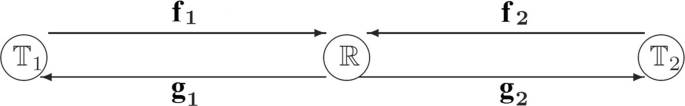
System configuration for two-way relay network. It shows a two-way relay network with two terminal nodes \(\mathbb {T}_{1}\) and \(\mathbb {T}_{2}\), and one relay node \(\mathbb {R}\). Each node has one antenna which cannot transmit and receive simultaneously. The channel from \(\mathbb {T}_{i}\) to \(\mathbb {R}\) is denoted as fi, whereas the one from \(\mathbb {R}\) back to \(\mathbb {T}_{i}\) is denoted as gi for i=1 and 2
If \(\mathbb {T}_{1}\) and \(\mathbb {T}_{2}\) add CP of length L, then the relay needs to carry out the operations of OFDM symbol timing synchronization, CP removal, and CP insertion. In order to simplify the tasks of the relay, \(\mathbb {T}_{1}\) and \(\mathbb {T}_{2}\) add CP of length 2L.

Abbreviations
- ACRB:
-
Approximated cramer-rao bound
- AF:
-
Amplify-and-forward
- AWGN:
-
Additive white Gaussian noise
- BER:
-
Bit error rate
- CIR:
-
Channel impulse response
- CP:
-
Cyclic prefix
- CSI:
-
Channel state information
- DA:
-
Data-aided
- DF:
-
Decode-and-forward
- DFT:
-
Discrete fourier transform
- HOS:
-
Higher order statistics
- IDFT:
-
Inverse discrete fourier transform
- i.i.d.:
-
Independent and identically distributed
- ISI:
-
Inter-symbol interference
- KCS:
-
Knowledge of the channel statistics
- LS:
-
Least squares
- MAP:
-
Maximum a posteriori
- ML:
-
Maximum likelihood
- MMSE:
-
Minimum mean square error
- MSE:
-
Mean square error
- OFDM:
-
Orthogonal frequency division multiplexing
- OWRN:
-
One-way relay network
- SISO:
-
Single-input single-output
- SNR:
-
Signal-to-noise ratio
- SOS:
-
Second-order statistics
- STC:
-
Space-time code
- TWRN:
-
Two-way relay network
- VC:
-
Virtual carrier
- ZP:
-
Zero padding
References
JN Laneman, DNC Tse, GW Wornell, Cooperative diversity in wireless networks: efficient protocols and outage behavior. IEEE Trans. Inf. Theory. 50(12), 3062–3080 (2004).
S Katti, S Gollakota, D Katabi, Embracing wireless interference: analog network coding. Comput. Sci. Artif. Intell. Lab. Tech. Rep (2007).
B Rankov, A Wittneben, Spectral efficient signaling for half-duplex relay channels. Annual Conference on Signals, Systems, and Computers, 1066–1071 (2005).
B Rankov, A Wittneben, Achievable rate regions for the two-way relay channel. International Symposium on Information Theory (ISIT), 1668–1672 (2006).
P Popovski, H Yomo, Wireless network coding by amplify-and-forward for bi-directional traffic flows. IEEE Commun. Lett. 11(1), 16–18 (2007).
T Cui, F Gao, T Ho, A Nallanathan, Distributed space-time coding for two-way wireless relay networks. International Conference on Communications (ICC), 3888–3892 (2008).
R Zhang, Y-C Liang, CC Chai, S Cui, Optimal beamforming for two-way multi-antenna relay channel with analogue network coding. IEEE J. Sel. Areas Commun. 27(5), 699–712 (2009).
C Xing, S Ma, Y-C Wu, Robust joint design of linear relay precoder and destination equalizer for dual-hop amplify-and-forward MIMO relay systems. IEEE Trans. Signal Process. 58(4), 2273–2283 (2010).
MW Baidas, AB MacKenzie, RM Buehrer, Network-coded bi-directional relaying for amplify-and-forward cooperative networks: a comparative study. IEEE Trans. Wirel. Commun. 12(7), 3238–3252 (2013).
P Hoeher, S Kaiser, P Robertson, Two-dimensional pilot symbol aided channel estimation by Wiener filtering. IEEE Int. Conf. Acoust. Speech Signal Process. (ICASSP). 3:, 1845–1848 (1997).
P Hoeher, S Kaiser, P Robertson, Pilot-symbol-aided channel estimation in time and frequency. IEEE Global Telecommunications Conference, 90–96 (1997).
Y Li, LJ Cimini, NR Sollenberger, Robust channel estimation for OFDM systems with rapid dispersive fading channels. IEEE Trans. Commun. 46(7), 902–915 (1998).
O Edfors, M Sandell, Beek van de JJ, SK Wilson, PO Borjesson, OFDM channel estimation by singular value decomposition. IEEE Trans. Commun. 46(7), 931–939 (1998).
O Edfors, M Sandell, Beek van de JJ, SK Wilson, PO Borjesson, Analysis of DFT-based channel estimators for OFDM. Wirel. Pers. Commun. 12(1), 55–70 (2000).
M Morelli, U Mengali, A comparison of pilot-aided channel estimation methods for OFDM systems. IEEE Trans. Sig. Process. 49(2), 3065–3073 (2001).
J Oliver, R Aravind, KMM Prabhu, Sparse channel estimation in OFDM systems by threshold-based pruning. IEEE Electron. Lett. 44(13), 830–832 (2008).
S Rosati, GE Corazza, A Vanelli-Coralli, OFDM channel estimation based on impulse response decimation: analysis and novel algorithms. IEEE Trans. Commun. 60(7), 1996–2008 (2012).
O Shalvi, E Weinstein, New criteria for blind deconvolution of non-minimum phase systems (channels). IEEE Trans. Inf. Theory. 36:, 312–321 (1990).
E Moulines, P Duhamel, JF Cardoso, S Mayrargue, Subspace methods for the blind identification of multichannel FIR filters. IEEE Trans. Sig. Process. 43(2), 516–525 (1995).
S Zhou, GB Giannakis, Finite-alphabet based channel estimation for OFDM and related multicarrier systems. IEEE Trans. Commun. 49(8), 1402–1414 (2001).
AP Petropulu, R Zhang, R Lin, Blind OFDM channel estimation through simple linear precoding. IEEE Trans. Wirel. Commun. 3(2), 647–655 (2004).
C Li, S Roy, Subspaced-based blind channel estimation for OFDM by exploiting virtual carriers. IEEE Trans Wirel. Commun. 2(1), 141–150 (2003).
B Su, PP Vaidyanathan, Subspace-based blind channel identification for cyclic prefix systems using few received blocks. IEEE Trans. Signal Process. 55(10), 4979–4993 (2007).
F Gao, Y Zeng, A Nallanathan, T-S Ng, Robust subspace blind channel estimation for cyclic prefixed MIMO OFDM systems: algorithm, identifiability and performance analysis. IEEE J. Sel. Areas Commun. 26(2), 378–388 (2008).
Y-C Pan, S-M Phoong, An improved subspace-based algorithm for blind channel identification using few received blocks. IEEE Trans. Commun. 61(9), 3710–3720 (2013).
B Su, Subspace-based blind and semiblind channel estimation in OFDM systems with virtual carriers using few received symbols. International Workshop on Signal Processing Advances in Wireless Communications (SPAWC), 100–104 (2014).
F Gao, R Zhang, Y-C Liang, Optimal channel estimation and training design for two-way relay networks. IEEE Trans. Commun. 57(10), 3024–3033 (2009).
F Gao, R Zhang, Y-C Liang, Channel estimation for OFDM modulated two-way relay networks. IEEE Trans. Signal Process. 57(11), 4443–4455 (2009).
L Sanguinetti, AA D’Amico, Y Rong, A tutorial on the optimization of amplify-and-forward MIMO relay systems. IEEE J. Sel. Areas Commun. 30(8), 1331–1346 (2012).
CWR Chiong, Y Rong, Y Xiang, Channel training algorithms for two-way MIMO relay systems. IEEE Trans. Signal Process. 61(16), 3988–3998 (2013).
S Abdallah, IN Psaromiligkos, Blind channel estimation for amplify-and-forward two-way relay networks employing M-PSK modulation. IEEE Trans. Signal Process. 60(7), 3604–3615 (2012).
Q Zhao, Z Zhou, J Li, B Vucetic, Joint semi-blind channel estimation and synchronization in two-way relay networks. IEEE Trans. Veh. Technol. 63(7), 3276–3293 (2014).
X Xie, M Peng, B Zhao, W Wang, Y Hua, Maximum a posteriori based channel estimation strategy for two-way relaying channels. IEEE Trans. Wirel. Commun. 13(1), 450–463 (2014).
X Liao, L Fan, F Gao, Blind channel estimation for OFDM modulated two-way relay network. Wireless Communications and Networking Conference (WCNC), 1–5 (2010).
T-C Lin, S-M Phoong, Blind channel estimation in OFDM-based amplify-and-forward two-way relay networks. IEEE International Conference on Acoustics, Speech, and Signal Processing (ICASSP) (2016).
M Morelli, U Mengali, A comparison of pilot-aided channel estimation methods for OFDM systems. IEEE Trans. Signal Process. 49(12), 3065–3073 (2001).
B Picinbono, Second-order complex random vectors and normal distributions. IEEE Trans. Signal Process. 44(10), 2637–2640 (1996).
HJ Larson, BO Shubert, Probabilistic Models in Engineering Sciences, Vols. I and II, first edition (Wiley, New York, 1979).
RA Horn, CR Johnson, Matrix Analysis (Cambridge University Press, Cambridge, 1985).
Funding
This work was supported by the Ministry of Science and Technology, Taiwan, R.O.C., under grant no. 106-2221-E-002-033.
Author information
Authors and Affiliations
Contributions
T-CL and S-MP constructed the theory. T-CL performed simulations and wrote a draft. S-MP modified the paper. Both authors read and approved the final manuscript.
Corresponding author
Ethics declarations
Competing interests
The authors declare that they have no competing interests.
Publisher’s Note
Springer Nature remains neutral with regard to jurisdictional claims in published maps and institutional affiliations.
Rights and permissions
Open Access This article is distributed under the terms of the Creative Commons Attribution 4.0 International License (http://creativecommons.org/licenses/by/4.0/), which permits unrestricted use, distribution, and reproduction in any medium, provided you give appropriate credit to the original author(s) and the source, provide a link to the Creative Commons license, and indicate if changes were made.
About this article

Cite this article
Lin, TC., Phoong, SM. A new blind algorithm for channel estimation in OFDM-based amplify-and-forward two-way relay networks. J Wireless Com Network 2018, 183 (2018). https://doi.org/10.1186/s13638-018-1193-3
Received:
Accepted:
Published:
DOI: https://doi.org/10.1186/s13638-018-1193-3