- Research
- Open access
- Published:
Energy-efficient power allocation for massive MIMO-enabled multi-way AF relay networks with channel aging
EURASIP Journal on Wireless Communications and Networking volume 2018, Article number: 206 (2018)
Abstract
In this paper, we consider a massive MIMO-enabled multi-way amplify-and-forward relay network with channel aging, where multiple users mutually exchange information via an intermediate relay equipped with massive antennas. For this system, we propose an energy-efficient power allocation scheme for the optimization of energy efficiency (EE). Specifically, we firstly derive accurate closed-form expressions of the system sum rate with aged channel state information (CSI) and predicted CSI. Secondly, based on the derived analytical results, a unified power allocation optimization problem with aged/predicted CSI is formulated for maximizing the system EE. To solve this challenging problem, the successive convex approximation technique is invoked to transform the original optimization problem into a tractable concave fractional programming problem. Then, Dinkelbach’s algorithm and Lagrangian dual method are adopted to find the optimal solution. In addition, to strike a balance between the computational complexity and the optimality, the EE maximization problem using the equal power allocation scheme is solved by extreme value theorem, leading to a closed-form optimal solution. Numerical results demonstrate the accuracy of our analytical results and the effectiveness of the proposed algorithms. Moreover, the impact of several important system parameters on the system performance achieved by the proposed algorithms is also illustrated.
1 Introduction
With the unprecedented growth of mobile data traffic volumes, the carbon emission of information and communication technologies is becoming an increasingly serious problem. Internationally, several academic and industrial research projects have been dedicated to maximize the overall network capacity and improve the energy efficiency (EE) of wireless communication systems (i.e., minimizing the amount of energy required to transmit data) [1–4]. More recently, as one of the major candidate technologies for fifth-generation (5G) wireless systems, massive multiple-input multiple-output (MIMO) has received tremendous attention from both academic and industry in wireless fields [5, 6].
More specifically, it was shown in [7] that massive MIMO systems (equipped with a very large number of antennas) are capable of achieving three orders of magnitude EE gains compared with single-antenna systems. The energy-efficient design of massive MIMO systems has emerged as a new research trend for 5G wireless communications [8, 9]. For example, in [10], the EE was analyzed in massive MIMO systems, under the effect of a general transceiver hardware impairments. In [11], the EE was maximized in a multi-user massive MIMO system, and the optimal system parameters (includes the number of base station (BS)’s antennas and users). In [12], the BS density, transmit power levels and number of antennas are optimized for maximizing EE in massive MIMO-enabled heterogeneous networks.
As another promising approach, multi-way relay networks (MWRNs) have recently received plenty of research interest [13, 14]. In general, as compared to one-way relay networks (OWRNs) and two-way relay networks (TWRNs), MWRNs are capable of achieving higher capacity and spectral efficiency (SE) and thus can be employed to effectively deal with the ever increasing demand for higher data rate and SE in a multi-user scenario. Therefore, the integration of massive MIMO and MWRN is regarded as a promising network architecture to meet the significant demand for mobile data applications. Additionally, it was shown in [15] that using simple relay transceivers (e.g., linear zero-forcing (ZF) transceiver), a multi-way MIMO relay system is capable of significantly alleviating the interference among different data streams/user equipments (UEs). Furthermore, similar to the observations in massive MIMO-enabled OWRNs [16] and TWRNs [17, 18], it was shown in [19] that by invoking a large-scale antenna array-equipped relay and a low-complexity ZF transceiver, the SE of MWRNs is also proportional to the number of relay antennas. At present, the existing related research on massive MIMO-enabled MWRNs mainly focused on analyzing the performance limits in various specific system configurations [19–24]. For instance, in [19], the asymptotic signal-to-interference-plus-noise ratio (SINR) of massive MIMO-enabled MWRNs was studied. Later on, the authors of [20] further analyzed the asymptotic SINR and average error rate performance and obtained the optimal pilot sequence length for maximizing the SE of multi-cell massive MIMO-enabled MWRNs. Moreover, the SE and asymptotic SINR of massive MIMO-enabled MWRNs are first analyzed with maximum-ratio processing, and then the same authors derived a closed form expression of the SE of massive MIMO-enabled MWRNs with ZF processing.
Moreover, prior works [19–22] considered the effect of channel imperfection due to channel estimation (CE), but ignored another important aspect of practical channel impairments known as channel aging, which refers to the phenomenon affected by the relative movement of users. This scenario is of high practical value in urban environments, where users move rapidly within a geographical area. Despite its significance, very few works have investigated its impact on the performance of massive MIMO systems. For point-to-point massive MIMO system, the impact of channel aging on the SINR performance was firstly studied by assuming matched filtering [25]. The impact of channel aging was lately investigated with ZF precoders [26] and minimum mean square error (MMSE) receivers [27]. For massive MIMO relay system, the asymptotic impact of channel aging on the performance of massive MIMO-enabled MWRNs was studied in [23]. Later on, the analysis was extended to the multi-cell massive MIMO-enabled MWRNs scenario for simultaneous wireless information and power transfer [24]. To the best of the authors’s knowledge, there is a paucity of contributions on energy-efficient transmission strategies of massive MIMO-enabled MWRNS, considering the effect of channel aging. It is challenging to extend the existing energy-efficient designs conceived for single-hop massive MIMO systems [10–12] to massive MIMO-enabled relay systems. Due to this fact, compared to single-hop transmission schemes, both signal processing schemes and the performance analysis of massive MIMO-enabled relay systems are fundamentally dependent on the more complex two-hop channels. Therefore, it is important to design energy-efficient transmission strategy for massive MIMO-enabled relay systems. Furthermore, the consideration of channel aging is of paramount importance because it can provide the robustness against the practical setting of user mobility that results to delayed and degraded channel state information (CSI).
Motivated by the above discussions, in this paper, we investigate low-complexity energy-efficient power allocation strategies for a massive MIMO-enabled MWRN with channel aging. Footnote 1 We assume that the CSI is estimated relying on the MMSE criterion, and the relay employs the low-complexity linear ZF transceivers. The main contributions of this paper are summarized as follows.
-
We respectively derive closed-form expression of the achievable sum rate (SR) for aged and predicted CSI, which enables us to efficiently evaluate the system performance, thus facilitating the energy-efficient power allocation strategies.
-
Based on the derived closed-form expressions, we formulate a unified optimization problem that optimizes power allocation of all UEs for maximizing the system EE, subject to limited transmit power, and minimum quality-of-service (QoS) constraints. Because of the intractable non-convexity of the formulated optimization problem, the successive convex approximation (SCA) technique is involved to transform the non-convex problem into a concave fractional programming (CFP) problem, which is then efficiently solved by Dinkelbach’s algorithm and Lagrangian dual method.
-
Furthermore, to strike a balance between the computational complexity and the optimality, a closed-form power control algorithm is provided under the assumption of equal power allocation (EPA) among multiple UEs, without requiring complicated iterative algorithms.
-
By simulation, the impact of the maximal transmit power, of the QoS constraint, and of the transmit power of each pilot symbol on the optimum EE is quantified. Moreover, our numerical results show that the EPA scheme-based power optimization strategies strike an attractive tradeoff between the achievable EE performance and the computational complexity imposed.
The remainder of this paper is organized as follows. The system model is described in Section 3. In Section 4, the closed-form expressions for SR are derived under aged and predicted CSI scenarios. In Section 5, we present the energy-efficient power allocation optimization problem under different performance criterions and constraints. The power allocation strategies are provided in Section 6, and the simulation results are given in Section 7. Finally, the conclusions are made in Section 8.
Notations: We use uppercase and lowercase boldface letters for denoting matrices and vectors, respectively. (·)∗, (·)T, and (·)H denote the conjugate, transpose, and conjugate transpose, respectively. ||·||, tr{·}, \(\mathbb {E}[\cdot ]\), Cov(·), and Var[·] stand for the Euclidean norm, the trace of matrices, the expectation, covariation, and variance operators, respectively. The diag{x} denotes a diagonal matrix with the vector x being its diagonal entries, and the operators modN(x) denote the modulo N of x. [A]i,j represents the entry at the i-th row and the j-th column of a matrix A. Finally, \(\mathcal {CN}(\mathbf {0},\mathbf {\Theta })\) denotes the circularly symmetric complex Gaussian distribution with zero mean and the covariance matrix Θ.
2 Method
This paper studies the energy-efficient power allocation problem of massive MIMO-enabled multi-way relay systems, under channel aging. The performance of the proposed framework was in depth examined through a series of simulation experiments including different system parameters, whereas the superiority of the proposed approach was clearly demonstrated by comparing it with other research works in the literature. Specifically, it has been shown that the different implementations of the proposed algorithm succeed in providing considerably higher EE in all different system settings while at the same time maintaining QoS at high levels. Moreover, the impact of normalized Doppler shifts fDTS (i.e., channel aging) on the system achievable rate is also illustrated. The simulation code was written in MATLAB.
3 System model and transmission scheme
As shown in Fig. 1, we consider a massive MIMO-enabled AF MWRN with non-pairwise ZF transmission,Footnote 2 where K spatially distributed single-antenna UEs (UEk, k∈{1,⋯,K}) exchange their information-bearing signals in K time slots among one another via a shared relay (R) equipped with M antennas.Footnote 3 Without loss of significant generality, we assume that the number of relay antennas is greater than the number of UEs served at the same time-frequency resources (i.e., M>K). The system operates over a bandwidth of B Hz and the channels are static within the time-frequency coherence blocks composed of T=BCTC data symbols, where BC and TC are the coherence bandwidth and coherence time, respectively. It is assumed that the channel coefficients do not change within one-symbol duration, but vary slowly from symbol to symbol. We assume that the relay operates on the half-duplex TDD mode. Each coherence interval is divided into three time phases, i.e., the CE phase, the multiple-access and broadcast phases. The multiple-access phase consists of only one time slot, whereas the broadcast phase contains K−1 time slots.
3.1 Data transmission
In the multiple-access phase, all K UEs simultaneously transmit their signals xU[ n] to the relay. These signals can be expressed as \(\mathbf {x}_{\mathrm {U}}[\!n]=\mathbf {P}_{\mathrm u}^{1/2}\mathbf {s}[\!n]\in \mathbb {C}^{K\times 1}\), where s[ n]=[s1[ n],…,sK[ n]]T is the information-bearing symbol vector with \(\mathbb {E}\left [\mathbf {s}[\!n]\mathbf {s}^{H}[\!n]\right ]=\mathbf {I}_{K}\) and Pu=diag{p1,⋯,pk,⋯,pK}, pk is the transmit power of the kth UE. The received signal \(\mathbf {y}_{\mathrm {R}}\in \mathbb {C}^{M\times 1}\) at the relay is given by
where \(\mathbf {G}[\!n]\in {\mathbb C}^{M\times K}\) represents the channel matrix from K UEs to the relay and nR[ n] denotes the additive white Gaussian noise (AWGN) that obeys \(\mathcal {CN}\left (\mathbf {0},\sigma _{\mathrm r}^{2}\mathbf {I}_{M}\right)\) at the relay.
To be specific, the channel matrix G[ n] can be expressed as
where \(\mathbf {H}[\!n]\in {\mathbb C}^{M\times K}\) is the small-scale fading (SSF) channel matrix and their entries obey independent identically distributed (i.i.d.) Gaussian distribution as \(\mathcal {CN}\left (0,1\right)\). D is a K×K diagonal matrix with [D]k,k=βk, which models the large-scale fading (LSF) capturing both path-loss and shadowing fading effects. Moreover, βk is assumed to remain constant for all n and is assumed to be known a priori as it changes very slowly compared with SSF channel coefficients.
In the broadcast phase, the relay simply performs transceive processing, which firstly detects the signals received and transmitted to all UEs in K−1 subsequent time slots. Here, we consider an intermediate jth (j∈{1,⋯,K−1}) time slot of the broadcast phase for the sake of exposition. In the context, the relay transmitted signal in the jth time slot of the broadcast phase is given by
where Fj[ n]=W2[ n]πjW1[ n] is the combined beamforming matrix at the relay, W1[ n] is a ZF detection matrix, and W2[ n] is a ZF precoding matrix. Moreover, πj is the permutation matrix employed at the relay in the jth time slot of the broadcast phase, which is designed to ensure that the kth (k∈{1,⋯,K}) UE, receives the signal from the k′th UE, with k′=modK(k+j). Specifically, πj is constructed as πj=(πo)j, and the K×K primary permutation matrix, πo, can be written as
where ek denotes a column vector of length K with 1 in the kth position and 0 in every other position. 𝜗j is the amplification factor designed to constrain the long-term relay transmit power pr, which is given as follows.
Then, the received signal vector at K UEs in the jth time slot of the broadcast phase can be written as follows.
where nu[ n] is the AWGN vector satisfying \(\mathbf {n}_{\mathrm {u}}[\!n]\sim {\mathcal {CN}}\left (\mathbf {0}, \sigma _{\mathrm {u}}^{2}\mathbf {I}_{K}\right)\). The aforementioned broadcast phase continues until the completion of all K−1 relay transmissions in K−1 consecutive time slots.
Substituting (1) and (3) into (6), the received signal at the kth UE in the jth time slot of the broadcast phase is expressed as
where gk[ n] is the k-th column of G[ n] and nu,k[ n] is the k-th element of nu[ n].
3.2 Channel estimation
The relay estimates the channel coefficients by transmitting orthogonal pilot sequences. All K UEs simultaneously transmit their pilot sequences of τr(τr≥K) symbols to the relay. The received pilot matrix at the relay is given by
where pp is the transmit power of each pilot symbol and \(\mathbf {Z}[\!n]\in {\mathbb {C}}^{M\times \tau _{\mathrm {r}}}\) is a noise matrix whose elements are i.i.d \({\mathcal {CN}}\left (0,\sigma _{\mathrm {r}}^{2}\right)\). \(\boldsymbol {\Phi }\in \mathbb {C}^{K\times \tau _{\mathrm {s}}}\) is the pilot sequence matrix transmitted from K UEs, satisfying ΦΦH=IK. Correlation of the received signal X[ n] with \(\frac {1}{\sqrt {\tau _{\mathrm {r}} p_{{\mathrm {p}}}}}\boldsymbol {\Phi }^{H}\) obtains
Therefore, the noisy observation of the channel vector from kth UE to the relay is expressed as
where \(\tilde {\mathbf {z}}_{k}[\!n]\) are the kth columns of the matrix \(\widetilde {\mathbf {Z}}[\!n]=\mathbf {Z}[\!n]\boldsymbol {\Phi }^{H}\). Since ΦΦH=IK, \(\tilde {\mathbf {z}}_{k}[\!n]\sim {\mathcal {CN}}\left (\mathbf {0},\sigma _{\mathrm r}^{2}\mathbf {I}_{M}\right)\).
Exploiting the MMSE criterion [28], the estimate of gk[ n], \(\widehat {\mathbf {g}}_{k}[\!n]\) is distributed as
where \(\widehat {\beta }_{k}=\frac {\tau _{{\mathrm {r}}}p_{{\mathrm {p}}}\beta _{k}^{2}}{\sigma _{\mathrm r}^{2}+{\mathrm \tau _{{\mathrm {r}}}}p_{{\mathrm {p}}}\beta _{k}}\).
Due to the orthogonality property of MMSE estimation, gk[ n] can be decomposed into
where \(\tilde {\mathbf {g}}_{k}[\!n]\sim {\mathcal {CN}}\left (\mathbf {0},\left ({\beta }_{k}-\widehat {\beta }_{k}\right)\mathbf {I}_{M}\right)\) is the CE error and is uncorrelated with \(\widehat {\mathbf {g}}_{k}[\!n]\).
3.3 Channel aging
To analyze the impact of channel aging, in our analysis, we adopt an autoregressive model of order 1 for approximating the temporally correlated fading channel coefficient. As such, the channel vectors for the k-th UE at time n+1 can be expressed as [25]
where \(\boldsymbol {\epsilon }_{k}[n+1]\sim \mathcal {CN}\left (\mathbf {0},\left (1-\alpha ^{2}\right)\beta _{k}\mathbf {I}\right)\) is a temporally uncorrelated complex Gaussian random process. We denote α=J0(2πfDTS) as a temporal correlation parameter, where J0(·) is the zero-order first-kind Bessel function. TS is the channel sampling duration and \(f_{\mathrm D}=\frac {vf_{c}}{c}\) is the maximum Doppler frequency shift, where v, fc, and c are the UEs’ velocity, carrier frequency, and the speed of light, respectively. Without loss of generality, we assume that all users move with the same velocity. As a result, the time variation does not depend on the user index. While this seems not realistic, we stay very near to the practical case by considering the worst-case scenario where we set all users with the velocity corresponding to the most varying user.
To this end, a model accounting for the combined effects of the CE error and channel aging effect can be expressed as
where \(\boldsymbol {\xi }_{{\mathrm {a}},k}[n+1]\sim {\mathcal {CN}}\left (\mathbf {0},\tilde {\beta }_{{\mathrm a},k}\mathbf {I}_{M}\right)\) is mutually independent of \(\bar {\mathbf {g}}_{{\mathrm {a}},k}[n+1]\sim {\mathcal {CN}}\left (\mathbf {0},\bar {\beta }_{{\mathrm {a}},k}\mathbf {I}_{M}\right)\) with \(\bar {\beta }_{{\mathrm {a}},k}=\alpha ^{2}\widehat {\beta }_{k}\), \(\tilde {\beta }_{{\mathrm a},k}\,=\,\beta _{k}-\alpha ^{2}\widehat {\beta }_{k}\). Obviously, the combined error ξa,k[n+1] consists of both the CE error and aged CSI effects.
3.4 Channel prediction
Channel prediction is an important approach to alleviate the channel aging effect [29–31]. In this subsection, we focus on predicting gk[n+1] based on the current and previous received training signals. The detailed procedure for predicting gk[n+1] is given as follows.
We adopt a Wiener predictor. Then, gk[n+1] is predicted according to \(\bar {\mathbf {x}}_{k}[\!n]\), where
with p being the predictor order. The predicted CSI is provided as follows.
where the optimal p-th linear Wiener predictor is given as [31]
Specifically, we have δ(p,α)=[1,α,⋯,αp] and
with
According to [30], the covariance matrix of \(\bar {\mathbf {g}}_{{\mathrm {p}},k}\left [n+1\right ]\) is given by α2Θk(p,α), where
Thus, the real channel can be decomposed as [31]
where ξp,k[n+1] is the channel prediction error vector with covariance matrix βkIM−α2Θk(p,α), which is independent of \(\bar {\mathbf {g}}_{{\mathrm p},k}\left [n+1\right ]\). According to [29], it can be obtained that
According to the result in ([31], Lemma 2), Θk(p,α) is a scaled identity matrix of size M×M, which can be straightforwardly shown as follows.
with \(\bar {\beta }_{{\mathrm p,}k}\,=\,\frac {1}{M}{\mathrm tr}\left (\alpha ^{2}\boldsymbol {\Theta }_{k}(p,\alpha)\right)\), \(\tilde {\beta }_{{\mathrm p,}k}\,=\,\frac {1}{M} {\text {tr}}\left (\beta _{k}\mathbf {I}_{M} \!-\right. \!\left.\alpha ^{2}\boldsymbol {\Theta }_{k}(p,\alpha)\right)\).
4 Performance analysis for achievable sum rate
In this section, we consider two different scenarios, i.e., aged and predicted CSI. We first provide a unified achievable SR expression for two scenarios. Next, we derive closed-form expressions for achievable SR under aged and predicted CSI scenarios, which are desirable for the subsequent energy-efficient optimization problem formulation.
We assume that the temporal correlation parameter α and the LSF channel matrix D are known a priori at the relay. Hence, we can have the following CSI
Then, the ZF-receive matrix W1[n+1] and ZF-transmit matrix W2[n+1] are respectively expressed as
where \(\bar {\mathbf {G}}[n+1]\triangleq [\bar {\mathbf {g}}_{1}[n+1],\cdots,\bar {\mathbf {g}}_{K}[n+1]]\).
After the imperfect self-interference cancelation (SIC), the received signal at the kth UE of the jth time slot of the broadcast phase can be rewritten as
where \(\lambda _{k}\,=\,\textbf {g}_{k}^{T}[n+1]\mathbf {F}_{j}[n+1]\textbf {g}_{k}[\!n]-\bar {\textbf {g}}_{k}^{T}[n+1]\mathbf {F}_{j}[n+1] \bar {\textbf {g}}_{k}[n+1]\) is the SIC coefficient for the kth UE.
From (26), the ergodic achievable rate of the kth UE in the jth time slot of the broadcast phase can be expressed as
where
with \({\mathrm DS}_{k}^{(j)}\triangleq \vartheta _{j}^{2}p_{k^{\prime }} \left |\mathbf {g}_{k}^{T}[n+1]\mathbf {F}_{j}[n+1]\mathbf {g}_{k^{\prime }}[n+1]\right |^{2}, {\mathrm RSI}_{k}^{(j)}\triangleq \vartheta _{j}^{2}p_{k}|\lambda _{k}|^{2}, {\mathrm NU}_{k}\triangleq \left |n_{{\mathrm u},k}[n+1] \right |^{2}, {\mathrm IUI}_{k}^{(j)}\triangleq \vartheta _{j}^{2}p_{i} \left |\mathbf {g}_{k}^{T}[n+1]\mathbf {F}_{j}[n+1]\mathbf {g}_{i}[n+1] \right |\) and \({\mathrm NR}_{k}^{(j)}\triangleq \vartheta _{j}^{2} \left |\mathbf {g}_{k}^{T}[n+1]\mathbf {F}_{j}[n+1]\mathbf {n}_{{\mathrm R}}[n+1] \right |\).
However, further derivation of (27) is difficult because of the intractability to carry out the ensemble average analytically. Instead, we adopt another technique to derive a worst-case lower bound of achievable rate. According to [32], we can rewrite \(y_{{\mathrm u},k}^{(j)}[n+1]\) as
with
In (29), the first part \(\vartheta _{j}\sqrt {p_{k^{\prime }}}\mathbb {E} \left [\mathbf {g}_{k}^{T}[n+1]\mathbf {F}_{j}[n+1]\right. \left.\mathbf {g}_{k^{\prime }}[n+1]\right ] s_{k^{\prime }}[n+1]\) is considered as “desired signal,” and the second term \(\tilde {n}_{k}[n+1]\) is considered as “effective noise,” uncorrelated with the first term. Therefore, by approximating the effective noise as independent Gaussian noise of the same variance [32], we can obtain the statistical CSI based achievable rate of the kth UE in the jth time slot of the broadcast phase as
with
where \(\text {SI}_{k}^{(j)}\), \(\text {UI}_{k}^{(j)}\), \(\text {NR}_{k}^{(j)}\), and NUk denote the residual self-interference after SIC, the inter-user interference, the amplified noise from the relay, and the noise at kth UE, respectively, i.e.,
Remark 1
The above worst-case lower bound of achievable rate in (31) is obtained by assuming that UEk uses only statistical information of the channel gains (i.e., \(\mathbb {E}\left [\mathrm {g}_{k}^{T}[n+1]\mathbf {F}_{j}[n+1]\mathbf {g}_{k^{\prime }}[n+1]\right ]\)) to decode the signal transmitted by \(UE_{k^{\prime }}\). By contrast, the ergodic rate in (27) is obtained by a sophisticated receiver, i.e., UEk knows perfectly \(\mathrm {g}_{k}^{T}[n+1]\mathbf {F}_{j}[n+1]\mathbf {g}_{k^{\prime }}[n+1]\). In Section 8, it is demonstrated via simulations that the performance gap between the achievable SRs given by (31) and (27) is rather small in massive MIMO-enabled MWRNs. It is clear that (31) is a very useful metric for obtaining the achievable rate in practical applications where CSI is not available.
Accordingly, the statistical CSI-based achievable SR of the considered system with aged and predicted CSI is uniformly given as
In the following theorems, two accurate closed-form expressions for the worst-case lower bound of achievable SR are derived under aged and predicted CSI scenarios.
Theorem 1
For ZF transceivers, with aged CSI, the worst-case lower bound of achievable SR in the considered massive MIMO-enabled MWRNs is given by
where the closed-form formula of \(\mathcal {R}_{\mathrm {a}k}^{(j)}\) is defined as
in which
where k′′=modK(K+k−j), i′′=modK(K+i−j), \(\mu _{1}=\frac {1}{M-K-1}\), \(\mu _{2}=\frac {(2+(M-K)(M-K-3))}{(M-K)(M-K-1)^{2}(M-K-3)}\) and \(\mathcal {A}_{\mathrm {a}j}={\sum \nolimits }_{k=1}^{K}\bar {\beta }_{\mathrm {a},k}^{-1}\bar {\beta }_{\mathrm {a},k^{\prime \prime }}^{-1}\).
Proof
Please see Appendix 1. □
For predicted CSI, a closed-form expression for the statistical CSI-based achievable SR is derived as follows.
Theorem 2
For ZF transceivers, with predicted CSI, the worst-case lower bound of achievable SR in the considered massive MIMO-enabled MWRNs is given by
where \(\widehat {\mathcal {R}}_{\mathrm {p}k}^{(j)}\) is derived as
in which
where \(\mathcal {A}_{\mathrm {p}j}={\sum \nolimits }_{k=1}^{K}\bar {\beta }_{\mathrm {p},k}^{-1}\bar {\beta }_{\mathrm {p},k^{\prime \prime }}^{-1}\).
Proof
Since the proof follows similar lines as the proof of Theorem 1, it is omitted. □
Remark 2
Through Theorems 1 and 2, two simple closed-form expression of the SR of the considered system have been derived. The advantage of these expressions are that it only depends on the LSF channel coefficients and the configurable system parameters. Thus, complicated calculations involving large-dimensional matrix variables that represent the SSF channel coefficients are avoided. In this way, the computational complexity which relates to the SSF-based signal processing is greatly reduced. It is underlined that these closed-form expressions establish an explicit functional relationship between the SR, the transmit powers of UEs, thus facilitating the introduction of the following novel energy-efficient resource allocation methodology.
5 EE optimization problem formulation
In the EE optimization, we employ a realistic power consumption model similar to those used in [11, 33]. The total power consumption of the considered system can be quantified as
where PPA is the power consumed by power amplifiers (PAs) given as
in which ηPA,U∈(0,1) and ηPA,R∈(0,1) are the efficiency of PAs at the UEs and at the relay, respectively. PC denotes the total circuit power consumption, to be more specific, we have
in which \(P_{\text {CE}}=M\frac {\log _{2}\left (\tau _{\mathrm {r}}\right)R_{\text {flops}}}{\eta _{\mathrm {C}}}\) is the power consumed for CE at the relay, Rflops is the floating-point operations per second (flops) per antenna for each user, and ηC is the power efficiency of computing measured in flops/W. \(P_{\text {LP}}=2M\frac {\left (K+K^{2}\right)R_{\text {flops}}}{\eta _{\mathrm {C}}}\) is the power consumed for the ZF-receive detector and ZF-transmit precoder. PRR is the other baseband processing power (such as ADC/DAC, modulation/demodulation) at each antenna, PcR and PcU are the power consumed at circuit components of each antenna at the relay and each UE, respectively, and Pf is the fixed power consumption at the relay.
The power consumption in (41) can be rewritten as
where \(\upsilon _{1}\triangleq \frac {\left (1-\frac {\tau _{\mathrm {r}}}{T}\right)}{\eta _{\mathrm {PA,U}}}\), \(P_{\text {fixed}}=\frac {\frac {\tau _{\mathrm {r}}}{T}Kp_{\mathrm {p}}}{\eta _{\mathrm {PA,U}}}+\frac {\left (1-\frac {\tau _{\mathrm {r}}}{T}\right)\left (K-1\right)p_{\mathrm {r}}}{\eta _{\text {PA},{\mathrm {R}}}}+KP_{\text {cU}}+P_{\text {CE}}+P_{\text {LP}}+M\left (P_{\text {RR}}+P_{\text {cR}}\right)+P_{\mathrm {f}}\).
Given the values of the other system parameters, the EE ηEE [bits/Joule] under aged and predicted CSI scenarios is unifiedly defined as
where
with \(\rho _{i,k}^{(j)}\), \(\mu _{k}^{(j)}\) are constant value (independent of transmit powers), which are different for aged CSI and predicted CSI. More precisely,
-
For aged CSI, \(\rho _{k,i}^{(j)}=p_{\mathrm {r}}\left (\mu _{1}\tilde {\beta }_{\mathrm {a},i}\bar {\beta }_{\mathrm {a},k^{\prime }}^{-1}+\mu _{1}\tilde {\beta }_{\mathrm {a},k}\bar {\beta }_{\mathrm {a},i^{\prime \prime }}^{-1}+\right. \left.\mu _{2}\tilde {\beta }_{\mathrm {a},i}\tilde {\beta }_{\mathrm {a},k}\mathcal {A}_{\mathrm {a}j}\right)+ \sigma _{\mathrm {u}}^{2}\left (\mu _{1}\bar {\beta }_{\mathrm {a},i^{\prime \prime }}^{-1}+\mu _{2}\tilde {\beta }_{\mathrm {a},i}\mathcal {A}_{\mathrm {a}j}\right)\), \(\mu _{k}^{(j)}=p_{\mathrm {r}}\left (\mu _{1}\sigma _{\mathrm {r}}^{2}\bar {\beta }_{\mathrm {a},k^{\prime }}^{-1}+\mu _{2}\sigma _{\mathrm {r}}^{2}\tilde {\beta }_{\mathrm {a},k}\mathcal {A}_{\mathrm {a}j}\right)+ \mu _{2}\sigma _{\mathrm {u}}^{2}\sigma _{\mathrm {r}}^{2}\mathcal {A}_{\mathrm {a}j}\).
-
For predicted CSI, \(\rho _{k,i}^{(j)}\,=\,p_{\mathrm {r}}\left (\mu _{1}\tilde {\beta }_{\mathrm {p},i}\bar {\beta }_{\mathrm {p},k^{\prime }}^{-1}+\mu _{1}\tilde {\beta }_{\mathrm {p},k}\bar {\beta }_{\mathrm {p},i^{\prime \prime }}^{-1}+\right. \left.\mu _{2}\tilde {\beta }_{\mathrm {p},i}\tilde {\beta }_{\mathrm {p},k}\mathcal {A}_{\mathrm {p}j}\right)+ \sigma _{\mathrm {u}}^{2}\left (\mu _{1}\bar {\beta }_{\mathrm {p},i^{\prime \prime }}^{-1}+\mu _{2}\tilde {\beta }_{\mathrm {p},i}\mathcal {A}_{\mathrm {p}j}\right)\), \(\mu _{k}^{(j)}=p_{\mathrm {r}}\left (\mu _{1}\sigma _{\mathrm {r}}^{2}\bar {\beta }_{\mathrm {p},k^{\prime }}^{-1}+\mu _{2}\sigma _{\mathrm {r}}^{2}\tilde {\beta }_{\mathrm {p},k}\mathcal {A}_{\mathrm {p}j}\right)+\mu _{2}\sigma _{\mathrm {u}}^{2}\sigma _{\mathrm {r}}^{2}\mathcal {A}_{\mathrm {p}j}\).
Remark 3
In (45), the pre-log factor \(\left (1-\frac {\tau _{\mathrm {r}}}{T}\right)\) is due to the fact that during each coherence interval of T symbols, we spend τr symbols for pilot-based CE. Moreover, the numerator K−1 of the pre-log factor \(\frac {K-1}{K}\) is due to the fact that any user node receives signals from other K−1 user nodes, while the denominator K follows by the single time slot in the multiple-access phase and K−1 time slots used for full-data exchange in the broadcast phase.
It is seen from (45) that the EE ηEE is a function of the transmit powers of K UEs, \(\left \{p_{k}\right \}_{k=1}^{K}\). How to wisely allocate the transmit power among the K UEs is crucial for achieving the optimum EE in the context of green communications. Hence, the energy-efficient power allocation is formulated as the following optimization problem:
where the objective function ηEE is defined by (45), and pmax is the maximum transmit power of each UE. The constraints C1 and C2 are the boundary values for the transmit powers of K UEs. The constraint C3 guarantees the transmission link quality by satisfying the minimum QoS requirement R0 for each UE at each time slot of the broadcast phase. Here, R0 denotes the required achievable rate for all UEs.
6 Energy-efficient power allocation algorithm
6.1 Optimal power allocation (OPA) scheme
It is easy to observe that (47) is not a CFP optimization problem, because the numerator of the objection function ηEE and the QoS constraints C3 are non-convex with respect to \(\left \{p_{k}\right \}_{k=1}^{K}\). Therefore, (47) cannot be directly solved by classic fractional programming tools. To overcome this difficulty, we employ the SCA technique proposed in [34–36] to sequently approximate \({\mathcal {R}}_{k}^{(j)}\) by using the following inequality:
The above inequation is tight at a particular value \(z_{k,j}=\bar {z}_{k,j}\) when the approximation constants ak,j and bk,j are chosen as
Motivated by the above convexity approximation, we employ the inequality (48) to approximate \(\widehat {\mathcal {R}}_{k}^{(j)}\), where zk,j corresponds to \(\phantom {\dot {i}\!}\widehat {\gamma }_{k,j}=\frac {p_{\mathrm {r}}p_{k^{\prime }}}{{\sum \nolimits }_{i=1}^{K}p_{i}\rho _{k,i}^{(j)}+\mu _{k}^{j}}\). Then, the variable change \(p_{k}=2^{q_{k}}\phantom {\dot {i}\!}\), for ∀k was used. Finally, we arrive at the following approximated optimization problem
where Q=diag{q1⋯,qk⋯,qK}, \(P_{\text {tot}}\left (\mathbf {Q}\right)=\upsilon _{1}\sum _{k=1}^{K}2^{q_{k}}+P_{\text {fixed}}\) and
with \(a_{k,j}=\frac {\bar {\gamma }_{k}^{(j)}}{1+\bar {\gamma }_{k}^{(j)}}\) and \(b_{k,j}=\log _{2}\left (1+\bar {\gamma }_{k}^{(j)}\right)-\frac {\bar {\gamma }_{k}^{(j)}}{1+\bar {\gamma }_{k}^{(j)}} \log _{2}\bar {\gamma }_{k}^{(j)}\) being the approximation constants computed as (49), where \(\bar {\gamma }_{k}^{(j)}=\frac {p_{\mathrm {r}}2^{q_{k^{\prime }}}}{{\sum \nolimits }_{i=1}^{K}2^{q_{i}}\rho _{k,i}^{(j)}+\mu _{k}^{j}}\). For any fixed ak,j and bk,j, it can be easily verified that (51) is convex with respect to \(\left \{ q_{k}\right \}_{k=1}^{K}\).Footnote 4 Therefore, the optimization problem (50) is a CFP problem with a quasi-concave objective function \(\widetilde {\eta }_{\text {EE}}(\mathbf {Q})\)Footnote 5 and convex constraints, which can be transformed into a convex optimization in a subtractive by the Dinkelbach’s method as follows [37].
where
Here, λ is a non-negative parameter, it can be noted that when λ→0, it implies that the energy-efficient problem (52) is degenerated to an optimization problem for the SE maximization. The optimal factor λ∗ (i.e., the optimal objective function value of (50)) works as the optimal EE for the system. For fixed parameters ak,j, bk,j, and λ, the optimization problem (52) is a convex optimization problem, which can be efficiently solved using standard convex optimization tools, e.g., CVX [38]. Next, we derive an iterative algorithm for solving this optimization by applying the Lagrangian dual method.
Thus, the dual problem associated with the primal problem (52) can be written as
where μ={μk},∀k are the Lagrangian multipliers associated with the transmit power constraints C2′. while ψ={ψk,j},∀k,j are the Lagrangian multipliers for QoS constraints C3′.
In the following, we solve the dual problem (54) using Lagrangian dual approach, which alternates between a subproblem (inner problem), updating the power allocation variables Q by fixing the Lagrangian multipliers μ, ψ, and a master problem (outer problem), updating the Lagrangian multipliers μ, ψ for the obtained solution of the inner problem Q∗. The Lagrangian dual approach is outlined as follows.
The optimization problem (54) is in a standard concave form, which can be efficiently solved by using standard optimization techniques and KKT conditions [38]. Thus, to obtain the optimal power allocation for users, we take the partial derivative of (54) with qk, k=1,⋯,K, and equate the results to zero, thus the power allocation at the (m+1)th iteration is updated as follows.
where [x]+= max{0,x}.
Since the dual problem in (54) is differentiable, the gradient method may be readily used for updating the Lagrangian dual variables μk and ψk,j,∀k,j as follows [39].
where ε1(m) and ε2(m) are the step sizes used for moving in the direction of the negative gradient for the Lagrangian multipliers μk and ψk,j, respectively. The updated Lagrange multipliers are used for updating the power allocation policy. We repeat this process until convergence. The detailed iterative procedure is summarized in Algorithm 1.

To get a better insight into the computational complexity of our proposed algorithm, we perform an exhaustive complexity analysis. First, it is assumed that the network factor λ converges in W iterations. The optimization problem (52) consists of K×(K−1) subproblems due to K UEs operating on K−1 effective time slots. Besides, the computational complexity resulted by these constraints C1′−C3′ is \({\mathcal {O}}\left (V^{3}+2\right)\), where V denotes each UE’s power level. Furthermore, the computational complexity of updating Lagrangian dual variables is given as \({\mathcal {O}}\left (K^{\varpi }\right)\) (for example ϖ=2 if the ellipsoid method is used [40]). Let us suppose if the dual objective function (54) converges in \(\mathcal {G}\) iterations, then the total complexity for the proposed OPA scheme becomes \({\mathcal {O}}\left (2W{\mathcal {G}}\left (K-1\right)(K)^{\varpi +2}\left (V^{3}+2\right)\right)\).
6.2 Equal power allocation (EPA) scheme
To strike a balance between the computational complexity and the optimality, we propose another lower-complexity power allocation scheme in this paper, i.e., an EPA scheme among all UEs. The same-level transmit powers of K UEs is set as pk=pu, for ∀k; then, the optimization problem (47) under the EPA scheme is simplified as
where
To solve the above optimization problem (58), we firstly find the feasible region of pu and then find the global extrema values. The detailed steps are shown as follows.
Firstly, we solve the Eq. \({\overline {\mathcal {R}}}_{k}^{(j)}\left (p_{\mathrm {u}}\right)={R}_{0}\) and get the solution \(p_{\mathrm {u},k,j}^{*}\) for ∀k,j. It can be easily determined that \({\overline {\mathcal {R}}}_{k}^{(j)}\left (p_{\mathrm {u}}\right)\) is a monotonically increasing function for pu. Hence, the QoS constraints of (58) can be reset as \(p_{\mathrm {u}}\geq p_{\mathrm {u},k,j}^{*}\) for ∀k,j, i.e.,
where \(p_{\mathrm {u,\max }}^{*}=\max \left \{p_{\mathrm {u,1,1}}^{*}\cdots,p_{\mathrm {u,}k,j}^{*},\cdots p_{\mathrm {u,}K,K-1}^{*}\right \} \). Considering both C5 and (61), the feasible region of pu for (58) becomes \(\left [p_{\mathrm {u},\max }^{*},p_{\max }\right ]\). If pu,max∗>pmax, the optimization problem becomes infeasible. Namely, there is no solution of pu satisfying the QoS constraints, so the algorithm should adjust pmax. If pu,max∗<pmax, (58) is feasible on \(\left [p_{\mathrm {u},\max }^{*},p_{\max }\right ]\).
Once feasible, we can find the global maximum of \(\overline {\eta }_{{\text {EE}}}\left (p_{{\mathrm {u}}}\right)\) in \(\left [p_{\mathrm {u},\max }^{*},p_{\max }\right ]\). To be more specific, it can be readily proved that \(\overline {\eta }_{{\text {EE}}}\left (p_{{\mathrm {u}}}\right)\) is quasi-concave in pu and therefore has a unique stationary point \(\overline {p}_{\mathrm {u}}\), which coincides with its global maximizer and can be found from the first-order derivative (i.e., \(\frac {\partial {\overline \eta }_{{\text {EE}}}\left (\overline {p}_{{\mathrm {u}}}\right)}{\partial \overline {p}_{\mathrm {u}}}=0\)). Then, since \(\overline {\eta }_{{\text {EE}}}\left (p_{{\mathrm {u}}}\right)\) is strictly increasing for \(p_{\mathrm {u}}\leq \overline {p}_{\mathrm {u}}\) and strictly decreasing for \(p_{\mathrm {u}}> \overline {p}_{\mathrm u}\). Therefore, the solution of (58), \(p_{\mathrm {u}}^{*}\) is obtained as follows.
Remark 4
Compared to the optimization problem (47), where K variables \(\left \{p_{k}\right \}_{k=1}^{K}\) are optimized, the new formulation (58) only uses pu as the optimization variable. Hence, the computational complexity of the EPA scheme in (58) is significantly lower than that of the OPA scheme solving (47). Moreover, the OPA scheme based (47) is solved by the iterative Dinkelbach’s algorithm and Lagrangian dual method, which requires a complexity of \({\mathcal {O}}\left (2W{\mathcal {G}}\left (K-1\right)(K)^{\varpi +2}\left (V^{3}+2\right)\right)\), the EPA scheme based (58) can obtain a closed-form optimal solution by comparing extreme values and boundary values of the optimization problem (58), without iteration. In contrast to OPA scheme, the computational complexity of the EPA scheme can be negligible.
7 Numerical results
In this section, we evaluate the EE performance of the considered massive MIMO-enabled MWRN that uses the proposed energy-efficient power allocation strategies, and demonstrate the accuracy of our analytical results as well as the impacts of several relevant parameters on the optimum EE via numerical simulations. Several key simulation parameters are set as Table 1 [11, 33]. Assume that the relay coverage area is modeled as a disc and the relay is located at the geometric center of the disc. Furthermore, all UEs are assumed to be randomly and uniformly distributed in the circular cell with a radius R, we assume that no UE is closer to the relay than Rmin, and the log-normal shadowing \(\xi _{k}\sim \ln {\mathcal {N}}\left (0,\sigma _{k}^{2}\right)\).
7.1 Accuracy of analytical results
In this subsection, we evaluate the accuracy of analytical results given in (35) with aged CSI, as well as in (38) with predicted CSI for different fDTS and p. We use normalized Doppler shifts fDTS to characterize channel aging. Larger normalized Doppler shifts correspond to large CSI delays (i.e., the more serious channel aging effect). We choose \(\sigma _{\mathrm {r}}^{2}=\sigma _{\mathrm {u}}^{2}=1\) and τr=K. For the clarity of analysis, we assume that the EPA scheme used at UEs is considered, i.e., pk=pu. All the simulated values are obtained by averaging over 106 independent Monte Carlo channel realizations.
Figure 2 shows the system’s achievable SR versus the number of antennas at the relay M for different normalized Doppler shifts fDTS. It can be clearly seen from Fig. 2 that the relative performance gaps between the analytical results (35) (marked as Analytical) and the simulated values (27) (marked as Simulated) are very small, which demonstrates analytical results’ accuracy. In addition, we can see a intuitive result that channel aging degrades the system’s achievable SR. Again, it is noted that increasing the number of relay antennas M improves the system’s achievable SR, as expected. This observation also implies that, when fDTS is relatively large, the contribution of the increasing of M diminishes quickly.

The system’s achievable SR versus the number of relay antennas M for different normalized Doppler shifts fDTS. K=20, pu=20 dBm, pr=40 dBm, and pp=40 dBm
We now investigate the benefits of channel prediction on the achievable SR in Fig. 3. As can be readily, our analytical results (38) are in perfect agreement with the simulated curves (27), demonstrating the accuracy of analytical results. In addition, it is noted that, as the normalized Doppler shift fDTS becomes large, the achievable SR loss increases significantly. Apparently, when the channel prediction order grows large, the achievable SR gain improves considerably. We also observe that, when the channel aging effect is less severe (i.e., fDTS is small), channel prediction becomes more important. Finally, it can be observed that, the predicted CSI case achieves a higher SR than the current CSI (no channel aging) case when fDTS is small, while its performance degrades substantially when fDTS is large and becomes worse than that with the current CSI case.

The system’s achievable SR versus the normalized Doppler shifts fDTS for different prediction order p. K=20, M=128, pu=20 dBm, pr=40 dBm, and pp=40 dBm
7.2 Optimality of the proposed optimization strategy
In Fig. 4, we show the convergence behavior of the proposed power allocation strategies (including both the OPA and the EPA schemes) under different channel prediction orders p. It can be observed that the EEs of the OPA scheme (by solving (47)) are monotonically increased with the iteration number, then converge to the optimal EE value after only a few iterations. In addition, in order to further demonstrate the effectiveness of the proposed schemes, a performance comparison is given with other algorithm (i.e., Charnes-Cooper transformation (CCT)-based method) for power allocation in [41]. From Fig. 4, we can observe that the OPA scheme with the CCT-based method is slightly superior to the proposed OPA scheme with lower iterations, but the CCT-based method involves perspective transformations, which increases the computational complexity.

Convergence and optimality of the proposed power allocation strategies, under different prediction orders p. pp=40 dBm, M=128, K=20, R0=4 bit/s/Hz, pmax=24 dBm and pr=40 dBm
At the same time, the lower-complexity EPA schemes for solving (58) achieve near-optimum performances, dispensing with any iteration. Moreover, it can be observed that the obtained EE performances of the EPA schemes are slightly worse those of the OPA schemes. Finally, in order to valid the accuracy of the derived lower bound and the optimality of the proposed power allocation strategies, in Fig. 4, we provide a performance benchmark that correspond to solving the problem (47) via the high-complexity brute-force searching relying on the ergodic achievable SR in (27). From Fig. 4, we can see that the EEs of the proposed methods are slightly inferior to the benchmarks, and this is mainly because the proposed schemes are sub-optimal methods which involve iterations and convex approximation. When using OPA scheme, K variables \(\left \{p_{k}\right \}_{k=1}^{K}\) must be optimized. By contrast, with EPA scheme, we only need to optimize the single variable pu. Furthermore, the OPA scheme obtains the optimal power allocation solution in virtue of the complicated iterative Dinkelbach’s algorithm and Lagrangian dual method. The EPA scheme can obtain a closed-form optimal solution by only comparing extreme values and boundary values of the optimization problem (58), without iteration. Hence, compared with the the OPA scheme, the computational complexity of the EPA scheme is significantly reduced. Therefore, the EPA scheme is a good choice in terms of the tradeoff between the achievable EE performance and the computational complexity. Finally, numerical results also reveal that higher prediction order can obtain the improvement of EE performance.
Figure 5 illustrates the optimum EE achieved by the proposed power allocation strategies versus the transmit power constraint pmax. It is observed that the OPA scheme slightly outperforms the EPA scheme in terms of the optimum EE achieved. Furthermore, we can see that, when pmax≤26 dBm, the optimum EEs achieved by these proposed schemes can be substantially improved as pmax increases. This observation suggests that at this region [10,26]dBm, increasing the available power budget is an energy-efficient choice. However, when pmax≥26 dBm, the optimum EEs of the proposed power allocation scheme converge to a certain stable level. This important observation suggests that, when pmax is large enough, the increasing of transmit power may not be a good choice from the perspective of EE. Finally, it is observed that the smaller fSTD achieves a higher EE for either power allocation strategy. This is rather expected, since the smaller fSTD means the less serious channel aging effect, and the EE loss becomes smaller accordingly.

The optimum EE versus the transmit power constraint, pmax, under different normalized Doppler shifts fDTS. K=20, M=128, pr=40 dBm, R0=4 bit/s/Hz and pp=40dBm
Figure 6 illustrates the impact of the QoS threshold R0 on the optimum EEs achieved by the proposed power allocation schemes. It can be readily noted that when R0≤ 4 bit/s/Hz, each optimum EE remains unchanged. This happens because when R0 takes small values, it is easy to satisfy the link’s QoS requirement. This observation suggests that, at the low QoS requirement region R0≤ 4 bit/s/Hz, we can make the best use of all the available power to achieve the maximum EE, without having to waste more power on unfavorable links. Meanwhile, when R0≥ 4 bit/s/Hz, the optimum EEs decrease as R0 increases. This is due to the fact that when R0 increases, an excess fraction of power has to be allocated to compensate for disadvantageous links, which results in a degradation of optimum EE. In other works, a higher minimum rate R0 is satisfied at the expense of a reduction of the optimum EE.

The optimum EE versus the QoS constraint, R0, under different normalized Doppler shifts fDTS. K=20, M=128, pr=40 dBm, pmax=24dBm and pp=40 dBm
In Fig. 7, we show the impact of the transmit power of each pilot symbol pp on the optimum EEs achieved by the proposed power allocation schemes. From these results and as it was expected, it can readily be observed that the the optimum EEs of all schemes increases with increasing pp. Moreover, as pp grows large, the growth of the achievable EE gradually slows down and saturates to the value that relies on perfect CSI estimation. This implies that although the system with high transmit power of each pilot symbol (i.e., pp=50 dBm) is capable of improving the CE accuracy, then achieves a better EE performance, the extremely high CE accuracy is not a wise choice at the cost of consuming more power.

The optimum EE versus the transmit power of each pilot symbol, pp, under different normalized Doppler shifts fDTS. K=20, M=128, pr=40 dBm, R0=4 bit/s/Hz, and pmax=24dBm
8 Conclusions
In this paper, we have provided the performance analysis of the system’s achievable SR and proposed low-complexity power allocation strategies for maximizing the EE of a massive MIMO-enabled MWRN with channel aging. Specifically, we derived closed-form expressions for the system’s achievable SR with/without channel prediction. Based on the derived analytical results, a unified power allocation optimization problem is established, under the transmit power and QoS constraints. Owing to the non-convexity of the objective function and QoS constraints, the original non-convex problem is sequently approximated as a solvable CFP problem with the aid of the SCA technique, which can be efficiently solved by the Dinkelbach’s algorithm and Lagrangian dual method. Moreover, we have proposed a closed-form power control algorithm for the lower-complexity EPA scheme. The impacts of normalized Doppler shifts fDTS, channel prediction order, and other relevant system parameters on the SR and EE performance are investigated via numerical simulations, which have verified the accuracy of our analytical results, and confirmed the effectiveness of the proposed power allocation schemes.
9 Appendix 1
10 Proof of Theorem 1
With aged CSI, \(\bar {\mathbf {g}}_{k}\left [n+1\right ]\sim {\mathcal {C}N}\left (\mathbf {0},\bar {\beta }_{{\mathrm a},k}\mathbf {I}_{K}\right)\) is independent of \({\boldsymbol \xi }_{{\mathrm a},k}\left [n+1\right ]\sim {\mathcal {C}N}\left (\mathbf {0},\tilde {\beta }_{{\mathrm a},k}\mathbf {I}_{K}\right)\).
where
with \({\widetilde {\mathbf {G}}}[n+1]=\left [{\boldsymbol {\xi }}_{{\mathrm {a}},1}[n+1],\cdots,{\boldsymbol {\xi }}_{{\mathrm {a}},K}[n+1]\right ]\).
-
Compute \(\varPsi _{1}^{(j)}\): According to the definition of Fj[n+1], we have
where \(\mu _{1}=\frac {1}{M-K-1}\) and k′′=modK(K+k−j). (a) results from the property Tr{AB}=Tr{BA}. As to the detailed derivation of (b), we use the identity as follows [44]: \(\boldsymbol {\Omega }\triangleq \left (\bar {{\mathbf {G}}}^{H}[n+1]\bar {\mathbf {G}}[n+1]\right)^{-1}\) is an inverted Wishart matrix, i.e., \({\boldsymbol {\Omega }}\sim {\mathcal {W}}_{K}^{-1}\left (M+K+1,\widehat {\mathbf {D}}_{{\mathrm {a}}}^{-1}\right)\)with \(\widehat {\mathbf {D}}_{{\mathrm {a}}}^{-1}={\text {diag}}\left \{ \bar {\beta }_{{\mathrm {a}},1}^{-1},\cdots,\bar {\beta }_{{\mathrm {a}},K}^{-1}\right \} \). Hence, we have [45]
-
Compute \(\varPsi _{2}^{(j)}\): Since \(\bar {\mathbf {G}}[n+1]\) and \(\widetilde {\mathbf {G}}[n+1]\) are independent, we
obtain
in which
where m′′=modK(K+m−j), \(\mu _{2}=\frac {(2+(M-K)(M-K-3))}{(M-K)(M-K-1)^{2}(M-K-3)}\) and \({\mathcal {A}}_{{\mathrm {a}} j}={\sum \nolimits }_{k=1}^{K}\bar {\beta }_{{\mathrm {a}},k}^{-1}\bar {\beta }_{{\mathrm {a}},k^{\prime \prime }}^{-1}\). The detailed derivation of (c) is given as follows [45]:
and for m≠k
According to (71) and (68), we get
-
Compute \(\varPsi _{3}^{(j)}\): Similarly, according to (68), we can obtain
Substituting (65), (71), and (72) into (8), we have
-
Derive \(\widehat {\mathcal {R}}_{k}^{(j)}\): From (31), we need to compute \({\mathbb E}\left [{\mathbf {g}}_{k}^{T}[n+1]\mathbf {F}_{j}[n+1]{\mathbf {g}}_{k^{\prime }}[n+1]\right ]\), \({\text {SI}}_{k}^{(j)}\), \({\text {UI}}_{k}^{(j)}\), \({\text {NR}}_{k}^{(j)}\), NUk, and \({\text {Var}}\left [{\mathbf {g}}_{k}^{T}[n+1]\mathbf {F}_{j}[n+1]\textbf {g}_{k^{\prime }}[n+1]\right ]\).
-
Compute \({\mathbb E}\left [{\mathbf {g}}_{k}^{T}[n+1]\mathbf {F}_{j}[n+1]{\mathbf {g}}_{k^{\prime }}[n+1]\right ]\): We have
with
where (d) results from the independence between \(\bar {\mathbf {g}}_{i}[n+1]\) and ξa,j[n+1] for ∀i,j. Hence, we have
-
Compute \({\mathrm Var}\left [\boldsymbol {{\mathrm {g}}}_{k}^{T}[n+1]\mathbf {F}_{j}[n+1]\mathbf {g}_{k^{\prime }}[n+1]\right ]\): According to the definition of variance, we have
where \(\varsigma _{k,j}=\mathbf {g}_{k}^{T}[n+1]\mathbf {F}_{j}[n+1]\mathbf {g}_{k^{\prime }}[n+1]\), \(\mathbb {E}\left [\left |\varsigma _{k,j}\right |^{2}\right ]\) can be decomposed into the following parts:
with
According to (77)–(79), we obtain
-
Compute \({\text {SI}}_{k}^{(j)}\): We have
where (e) results from the property \(\bar {\mathbf {g}}_{k}^{T}[n+1] \mathbf {F}_{j}[n+1] \bar {\mathbf {g}}_{k}[n+1]={\boldsymbol {e}}_{k}^{T}{\boldsymbol {\pi }}_{j}{\boldsymbol {e}}_{k}=0\), and
Substituting (82) into (81), we obtain
-
Compute \({\text {UI}}_{k}^{(j)}\): Following the same methodology used for computing \(\mathbb {E}\left [|\lambda _{k}|^{2}\right ]\), we can easily derive
with
where i′′=modK(K+i−j).
According to (84) and (85), we can obtain
Therefore, we can conclude
-
Compute \({\mathrm NR}_{k}^{(j)}\): We have
with
Substituting (90) into (89), we can obtain
-
Compute NUk: We have
Substituting (73), (76), (80), (83), (88), (91), and (92) into (32), we can obtain (35) after some simple algebraic manipulations. Thus, the proof of Theorem 1 is complete.
Notes
Although we respectively studied the resource allocation for EE maximization in the massive MIMO-enabled OWRNs and MWRNS in [42, 43], the works in [42, 43] only considered the channel estimation (CE) error and ignored the effect of channel aging. Contrast to the transmission schemes proposed in [42, 43], the performance analysis and power allocation algorithms in this paper have stronger robustness over the practical communication scenario.
This setup is general enough to model a variety of communication scenarios. Certain practical applications such as multimedia teleconferencing via a satellite or mutual data exchange between sensor nodes and the data fusion center in wireless sensor networks require mutual data exchange among more than just two terminals.
Fig. 1 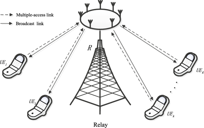
An illustration of the massive MIMO-enabled MWRN model in which the relay helps multiple users to simultaneously exchange messages
In this paper, for simplicity and tractability, we assumed that the direct link between any two UEs is ignored due to severe path loss. This assumption has been widely made in multi-way relay systems [13, 14], and it is easily extended to complex system models with a direct communication link between two UEs.
The log-sum-exp is convex [38].
The numerator is concave, and the denominator is convex [38].

Abbreviations
- 5G:
-
Fifth-generation
- AWGN:
-
Additive white Gaussian noise
- BS:
-
Base station
- CCT:
-
Charnes-Cooper transformation
- CE:
-
Channel estimation
- CFP:
-
Concave fractional programming
- CSI:
-
Channel state information
- EE:
-
Energy efficiency
- EPA:
-
Equal power allocation
- LSF:
-
Large-scale fading
- MIMO:
-
Multiple-input multiple-output
- MMSE:
-
Minimum mean square error
- MWRN:
-
Multi-way relay network
- OPA:
-
Optimal power allocation
- OWRN:
-
One-way relay network
- QoS:
-
Quality-of-service
- SCA:
-
Successive convex approximation
- SE:
-
Spectral efficiency
- SINR:
-
Signal-to-interference-plus-noise ratio
- SR:
-
Sum rate
- SSF:
-
Small-scale fading
- TWRN:
-
Two-way relay network
- UE:
-
User equipment
- ZF:
-
Zero-forcing
References
I. Chih-Lin, C. Rowell, S. Han, Z. Xu, G. Li, Z. Pan, Toward green and soft: a 5G perspective. IEEE Commun. Mag. 52(2), 66–73 (2014).
Z. Hasan, H. Boostanimehr, V. Bhargava, Green cellular networks: a survey, some research issues and challenges. IEEE Commun. Surv. Tutorials. 13(4), 524–540, Fourth Quarter (2011).
C. Han, T. Harrold, S. Armour, I. Krikidis, S. Videv, PM. Grant, H. Haas, J. Thompson, I. Ku, CX. Wang, TA. Le, M. Nakhai, J. Zhang, L. Hanzo, Green radio: radio techniques to enable energy-efficient wireless networks. IEEE Commun. Mag. 49(6), 46–54 (2011).
Y. Chen, S. Zhang, S. Xu, G. Li, Fundamental trade-offs on green wireless networks. IEEE Commun. Mag. 49(6), 30–37 (2011).
F. Rusek, D. Persson, BK. Lau, E. Larsson, T. Marzetta, O. Edfors, F. Tufvesson, Scaling up MIMO: opportunities and challenges with very large arrays. IEEE Signal Process. Mag. 30(1), 40–60 (2013).
EG. Larsson, O. Edfors, F. Tufvesson, TL. Marzetta, Massive MIMO for next generation wireless systems. IEEE Commun. Mag. 52(2), 186–195 (2014).
HQ. Ngo, E. Larsson, T. Marzetta, Energy and spectral efficiency of very large multiuser MIMO systems. IEEE Trans. Commun. 61(4), 1436–1449 (2013).
L. Lu, G. Y. Li, A. L. Swindlehurst, A. Ashikhmin, R. Zhang, An overview of massive MIMO: benefits and challenges. IEEE J. Sel. Topics Signal Process. 8(5), 742–758 (2014).
S. Buzzi, I. Chih-Lin, T. E. Klein, H. V. Poor, C. Yang, A. Zappone, A survey of energy-efficient techniques for 5G networks and challenges ahead. IEEE J Sel. Areas in Commun. 34(4), 697–709 (2016).
E. Björnson, J. Hoydis, M. Kountouris, M. Debbah, Massive mimo systems with non-ideal hardware: energy efficiency, estimation, and capacity limits. IEEE Trans. Inf. Theory. 60(11), 7112–7139 (2014).
E. Bjornson, L. Sanguinetti, J. Hoydis, M. Debbah, Optimal design of energy-efficient multi-user MIMO systems: Is massive MIMO the answer?IEEE Trans. Wireless Commun. 14(6), 3059–3075 (2015).
E. Björnson, L. Sanguinetti, M. Kountouris, Deploying dense networks for maximal energy efficiency: small cells meet massive mimo. IEEE J. Sel. Areas Commun. 34(4), 832–847 (2016).
D. Gündüz, A. Yener, A. Goldsmith, HV. Poor, The multiway relay channel. IEEE Trans. Inf. Theory. 59(1), 51–63 (2013).
Y. Tian, A. Yener, in Proc. IEEE Int. Symp. on Inf. Theory (ISIT). Degrees of freedom for the MIMO multi-way relay channel (IEEEIstanbul, 2013), pp. 1576–1580.
G. Amarasuriya, C. Tellambura, M. Ardakani, Multi-way MIMO amplify-and-forward relay networks with zero-forcing transmission. IEEE Trans. Commun. 61(12), 4847–4863 (2013).
H. A. Suraweera, H. Q. Ngo, T. Q. Duong, C. Yuen, E. G. Larsson, in Proc. IEEE Int. Conf. on Commun. (ICC). Multi-pair amplify-and-forward relaying with very large antenna arrays (IEEEBudapest, 2013), pp. 1–6.
H. Cui, L. Song, B. Jiao, Multi-pair two-way amplify-and-forward relaying with very large number of relay antennas. IEEE Trans. Wireless Commun. 13(5), 2636–2645 (2014).
S. Jin, X. Liang, K-K. Wong, X. Gao, Q. Zhu, Ergodic rate analysis for multipair massive MIMO two-way relay networks. IEEE Trans. Wireless Commun. 14(3), 1480–1491 (2015).
G. Amarasuriya, H. V. Poor, in Proc 2014 IEEE 25th Annual, Int. Symp. on Personal, Indoor, and Mobile Radio Commun. (PIMRC). Multi-way amplify-and-forward relay networks with massive MIMO (IEEEWashington DC, 2014), pp. 595–600.
Kudathanthirige D.P., G. A. A Baduge, Multicell multiway massive MIMO relay networks. IEEE Trans. Veh. Technol. 66(8), 6831–6848 (2017).
C. D. Ho, H. Q. Ngo, M. Matthaiou, T. Q. Duong, in Proc. IEEE Int. Conf. on Recent Advances in Signal Processing, Telecommunications Computing (SigTelCom). Multi-way massive MIMO relay networks with maximum-ratio processing (IEEEDa Nang, 2017), pp. 124–128.
C. D. Ho, H. Q. Ngo, M. Matthaiou, T. Q Duong, On the performance of zero-forcing processing in multi-way massive MIMO relay networks. IEEE Commun.Lett. 21(4), 849–852 (2017).
G. Amarasuriya, H. V. Poor, in Proc 2015 IEEE Int. Conf. on Commun. (ICC). Impact of channel aging in multi-way relay networks with massive MIMO (London, UK, 2015), pp. 1951–1957.
G. Amarasuriya, E. G. Larsson, H. V. Poor, Wireless information and power transfer in multiway massive MIMO relay networks. IEEE Trans. Wireless Commun. 15(6), 3837–3855 (2016).
K. T. Truong, R. W. Heath, Effects of channel aging in massive MIMO systems. J. Commun. and Netw. 15(4), 338–351 (2013).
A. K. Papazafeiropoulos, T. Ratnarajah, in Proc. IEEE Wireless Commun. and Netw. Conf. (WCNC). Linear precoding for downlink massive MIMO with delayed CSIT and channel prediction (IEEEIstanbul, 2014), pp. 809–914.
A. K. Papazafeiropoulos, T Ratnarajah, in Proc. IEEE Conf. on Acoustics, Speech and Signal Process. (ICASSP). Uplink performance of massive MIMO subject to delayed CSIT and anticipated channel prediction (IEEEFlorence, 2014), pp. 3162–3165.
H. Q. Ngo, H. Suraweera, M. Matthaiou, E. Larsson, Multipair full-duplex relaying with massive arrays and linear processing. IEEE J. Sel. Areas Commun. 32(9), 1721–1737 (2014).
S Zhou, G. B Giannakis, How accurate channel prediction needs to be for transmit-beamforming with adaptive modulation overrayleigh MIMO channels?IEEE Trans. Wireless Commun. 3(4), 1285–1294 (2004).
A. K. Papazafeiropoulos, T. Ratnarajah, Deterministic equivalent performance analysis of time-varying massive MIMO systems. IEEE Trans. Wireless Commun. 14(10), 5795–5809 (2015).
C Kong, C. Zhong, A. K. Papazafeiropoulos, M. Matthaiou, Zhang Z, Sum-rate and power scaling of massive MIMO systems with channel aging. IEEE Trans. Commun. 63(12), 4879–4893 (2015).
J. Jose, A. Ashikhmin, T. L. Marzetta, S Vishwanath, Pilot contamination and precoding in multi-cell TDD systems. IEEE Trans. Wireless Commun. 10(8), 2640–2651 (2011).
W. Liu, A. Zappone, C. Yang, E. Jorswieck, in Proc. IEEE Int. Works. on Signal Process in Advances in Wireless Commun. (SPAWC). Global EE optimization of massive MIMO systems (IEEEStockholm, 2015), pp. 221–225.
B. R. Marks, G. P. Wright, A general inner approximation algorithm for nonconvex mathematical programs. Oper. Res. 26(4), 681–683 (1978).
J. Papandriopoulos, J. S. Evans, Scale: a low-complexity distributed protocol for spectrum balancing in multiuser DSL networks. IEEE Trans. Inf. Theory. 55(8), 3711–3724 (2009).
A. Zappone, E. Jorswieck, Energy efficiency in wireless networks via fractional programming theory. Found. Trends Commun. Inf. Theory. 11(3–4), 185–396 (2015).
W Dinkelbach, On nonlinear fractional programming. Manag. Sci. 13(7), 492–498 (1967).
S. Boyd, L. Vandenberghe, Convex optimization (Cambridge University Press, Cambridge, United Kingdom, 2004).
W. Yu, R Lui, Dual methods for nonconvex spectrum optimization of multicarrier systems. IEEE Trans. Commun. 54(7), 1310–1322 (2006).
H. Zhang, Y. Liu, M. Tao, Resource allocation with subcarrier pairing in OFDMA two-way relay networks. IEEE Wireless Commun. Lett. 1(2), 61–64 (2012).
M. Naeem, K. Illanko, A. Karmokar, A. Anpalagan, M Jaseemuddin, Decode and forward relaying for energy-efficient multiuser cooperative cognitive radio network with outage constraints. IET Commun. 8(5), 578–586 (2014).
F. Tan, T. Lv, S Yang, Power allocation optimization for energy-efficient massive MIMO aided multi-pair decode-and-forward relay systems. IEEE Trans. Commun. 65(6), 2368–2381 (2017).
F. Tan, T. Lv, P. Huang, Global energy efficiency optimization for wireless-powered massive MIMO aided multiway af relay networks. IEEE Trans, Signal Process. 66(9), 2384–2398 (2018).
K. V. Mardia, JT. Kent, J. M. Bibby, Multivariate analysis (Academic press, London, United Kingdom, 1979).
Inverse Wishart distribution (2018). Available https://en.wikipedia.org/wiki/Inverse-Wishartdistribution.
Funding
This work was supported by the National Natural Science Foundation of China (61471135, 61671165); the Guangxi Natural Science Foundation (2016GXNSFGA380009); the PhD Research Startup Fund of Guilin University of Electronic Technology (UF17048Y); the Fund of Key Laboratory of Cognitive Radio and Information Processing (Guilin University of Electronic Technology), China; and the Guangxi Key Laboratory of Wireless Wideband Communication and Signal Processing (CRKL160105, CRKL170101).
Author information
Authors and Affiliations
Contributions
FT was responsible for mathematical derivation, numerical simulation, and paper writing. HC was responsible for problem formulation and paper revision. FZ was responsible for problem and result discussion. XL was responsible for model validation and result check. All authors read and approved the final manuscript.
Corresponding author
Ethics declarations
Competing interests
The authors declare that they have no competing interests.
Publisher’s Note
Springer Nature remains neutral with regard to jurisdictional claims in published maps and institutional affiliations.
Additional information
Authors’ information
Fangqing Tan received the M.Eng. degree in communication and information systems from Chongqing University of Post and Telecommunications, China, in 2012, and the Ph.D. degree in communication and information systems from Beijing University of Posts and Telecommunications, China, in 2017. He is currently a lecturer with the School of Information and Communication, Guilin University of Electronic Technology, Guilin, China. His research interests include massive MIMO systems, cooperative communications, and energy-efficient wireless communications. Hongbin Chen received the B.Eng. degree in electronic and information engineering from Nanjing University of Posts and Telecommunications, Nanjing, China, in 2004 and the Ph.D. degree in circuits and systems from South China University of Technology, Guangzhou, China, in 2009. From October 2006 to May 2008, he was a Research Assistant with the Department of Electronic and Information Engineering, Hong Kong Polytechnic University, Hong Kong. From March to April 2014, he was a Research Associate with the same department. From May 2015 to May 2016, he was a Visiting Scholar with the Department of Electrical and Computer Engineering, National University of Singapore, Singapore. He is currently a Professor with the School of Information and Communication, Guilin University of Electronic Technology, Guilin, China. His research interests include energy-efficient wireless communications. Feng Zhao received the Ph.D. degree in communication and information systems from Shandong University, China in 2007. Now, he is a Professor with the School of Information and Communication, Guilin University of Electronic Technology, China. His research interests include wireless communications, signal processing, and information security. Xiaohuan Li received the B.Eng. and M.Sc. degrees from Guilin University of Electronic Technology, China, in 2006 and 2009, respectively, and the Ph.D. degree from South China University of Technology, China, in 2015. He is currently an Associate Professor with the School of Information and Communication, Guilin University of Electronic Technology, China. His research interests include vehicular ad hoc networks.
Rights and permissions
Open Access This article is distributed under the terms of the Creative Commons Attribution 4.0 International License(http://creativecommons.org/licenses/by/4.0/), which permits unrestricted use, distribution, and reproduction in any medium, provided you give appropriate credit to the original author(s) and the source, provide a link to the Creative Commons license, and indicate if changes were made.
About this article

Cite this article
Tan, F., Chen, H., Zhao, F. et al. Energy-efficient power allocation for massive MIMO-enabled multi-way AF relay networks with channel aging. J Wireless Com Network 2018, 206 (2018). https://doi.org/10.1186/s13638-018-1222-2
Received:
Accepted:
Published:
DOI: https://doi.org/10.1186/s13638-018-1222-2