Optimizing radio resources for multicasting on high-altitude platforms

Abstract

High-altitude platforms (HAPs) are quasi-stationary aerial wireless communications platforms meant to be located in the stratosphere, to provide wireless communications and broadband services. They have the ability to fly on demand to temporarily or permanently serve regions with unavailable infrastructure. In this paper, we consider the development of an efficient method for resource allocation and controlling user admissions to multicast groups in a HAP system. Power, frequency, space and time domains are considered in the problem. The combination of these many aspects of the problem in multicasting over an OFDMA HAP system were not, to the best of our knowledge, addressed before. Due to the strong dependence of the total number of users that could join different multicast groups on the possible ways we may allocate resources to the different multicast groups, it is important to consider a joint user to multicast group assignments and radio resource management across the groups. From the service provider’s point of view, it would be in its best interest to be able to admit as many users as possible, while satisfying their quality of service requirements.

The problem turns out to be a mixed integer non-convex non-linear program for which branch and bound solution framework is guaranteed to solve the problem. Branch and bound (BnB) can be also used to obtain sub-optimal solutions with desired quality. Even though branch and bound is guaranteed to find the optimal solution, the computational cost could be extremely high, which is why we considered different types of enhancements to BnB. Mainly, we consider reformulations by linearizing a specific set of quadratic constraints in the derived formulation, as well as the application of different branching techniques to find the one that performs the best. Based on the conducted numerical experiments, it was concluded that linearization, applied for at least 100 presolving rounds, and cloud branching achieve the best performance.

1 Introduction to high-altitude platforms

Delivering high-capacity services over wireless medium presents challenges, since the spectrum is limited and the demand for its access is constantly growing. For terrestrial cellular networks, the solution is to decrease the transmission range of a base station (BS) and deploy more base stations which require backhaul interconnections. Clearly, this is a costly and difficult proposition, especially for areas with hostile geographical nature. This pressure on the radio spectrum requires moving higher in frequency to K/Ka bands (26–40 Ghz), which are less heavily congested and can provide significant bandwidth. The main problem with working in K/Ka bands is that line-of-sight (LOS) or quasi-LOS propagation is needed [1].

The visibility problem can be solved using satellite technology, which is a well-established alternative to terrestrial infrastructures that is able to serve wide areas with a cellular coverage, thus implementing frequency reuse paradigms. Geostationary Earth orbit (GEOs) satellites are located at about 36 thousand kilometers away from the earth’s surface. Due to the large distance from the earth’s surface, GEOs have huge antenna footprints that can cover entire continents providing services to millions of users. However, being far away from the earth’s surface also has major drawbacks, mainly due to the very critical free-space path loss and large propagation delays. The solution to these problems require large antennas and sophisticated architectures and protocols at the customer receivers. Furthermore, technological constraints for on-board antennas prevent the possibility of optimizing the cell dimension on the ground, thus potentially lowering frequency reuse efficiency and, consequently, overall capacity. Another type of satellites is the Low Earth Orbit (LEO) satellites which overcomes many of the drawbacks specific to GEO satellites as they are much nearer to the earth’s surface (200–1600 km). However, a single LEO satellite based system would not be suitable for real-time transmission since the satellite is frequently out of visibility. In such a system, only store and forward techniques could be used. If continuous coverage is required, then an entire constellation of LEO satellites must be used. Obviously this is too costly, and necessitates that efficient handover schemes be used among the satellites.

A potential solution for these problems that has been adopted is carrying communications relay payloads and operating in a quasi-stationary position in the stratosphere layer of the atmosphere. LOS propagation paths can be provided to most users, with modest free space path loss and propagation delays, thus enabling services that take advantage of the best features of both wireless terrestrial and satellite communications. The platforms that carry these payloads were called high-altitude platforms (HAPs) [2].

HAPs are quasi-stationary aerial platforms that are meant to be located at a height of 17–22 km above earth’s surface in the stratosphere layer. Many of their pros are a combination of those in both, terrestrial wireless and satellite communication systems. Some of those pros are [3]:

• Their ability to fly on demand to temporarily or permanently serve regions with unavailable telecommunications infrastructure.

• A single HAP has a large area coverage that can go up to 150 km compared to a single terrestrial cellular base station (BS) whose maximum radius, for macro cells, is in the range of 20–30 km.

• Low propagation delays compared to satellites which implies better perceived quality of service (QoS) by the users for real-time applications like voice and video.

• Stronger received signal strengths as compared to satellites and hence user terminals need not be bulky.

• Deployment time is low since one platform and ground support are sufficient to start the service.

• Much less ground-based infrastructure compared to terrestrial cellular networks.

For the same allocated bandwidth in a specified area, terrestrial systems require a large number of base stations. On the other hand, GEO satellites have cell size limitations due to large footprints on the earth’s surface and non-geostationary satellites face handover problems and the need to deploy the entire constellation, thus requiring high launching costs to place them in orbits. In this case, HAPs seem to be an attractive choice.

2 Recent works in HAPs

Among the recent works in the area of HAPs, is the work done by Sudheesh et al. in [4]. In their paper, they show how spatial multiplexing could be performed to boost the spectral efficiency. They state that in a single HAP system with multiple antennas on-board, spatial multiplexing cannot typically be achieved due to high correlation between paths. Therefore, they proposed the use of multiple spatially separated HAPs to perform precise beamforming. Due to the high altitudes and imperfect stabilization, it is challenging to acquire accurate channel state information (CSI), that is necessary for precise beamforming. For this, the authors realize an interference alignment technique based on a multiple antenna tethered balloon that could be deployed and used as a relay between the multiple HAPs and the ground stations. In particular, a multiple-input multiple-output X network was considered in [4], and the capacity for that network was obtained in close form. The authors showed that a maximum sum-rate was obtained.

In [5], Xu et al. proposed a geometry based HAP channel model that considers the statistical and geometry properties of terrestrial environments comprehensively for the purpose of efficient deployment of HAPs. Based on their proposed channel model, they also derived the LOS transmission probability of air-to-ground communication and performed the analysis for the path loss. They also proposed an algorithm that maximizes the efficiency, in terms of the ratio of the radius of HAP footprint to inter-HAP distance. In [6], Dong et al. treated HAPs as mobile base stations and considered a method for their placement with guarantees on QoS and user demands in a constellation of multiple interconnected HAPs. They established QoS metrics by considering the information isolation, integrity, rate and availability. The user demand has been modeled by considering the broadband size, the population distribution density, and scale factor of the HAP network users. Based on the network coverage model, they gave out the design vector of HAPs layout optimization, i.e., number of HAPs, downlink antenna area, power of payload, longitude of HAP and latitude of HAP. Moreover, in [6] a nonlinear, nonconvex, and non-continuous combinatorial optimization model was proposed. This was solved by an improved artificial immune algorithm.

In [7], Zhang et al. considered UAV-enabled mobile relaying. They studied a system in which a UAV is deployed to assist in the information transmission from a ground source to a ground destination with their direct link blocked. In their paper, they study two problems, spectrum efficiency and energy efficiency maximization for that system and revealed their trade-off with the UAV’s propulsion energy taken into account. The type of motion that they considered is circular, and the type of relaying is a decode and forward in a time-division duplex mode. They derived the optimal solutions for both problems and showed that energy efficiency maximization requires a larger circular trajectory radius than spectral efficiency maximization. Their numerical results showed performance gain for mobile relay in circular trajectory over static relaying with a fixed relay.

In [8], the design of an active electronically steerable antenna array (AESA) enabling broadband line-of-sight communication from HAPs was investigated. The array is constructed using a multitude of single chip multi-channel beamforming modules capable of switched bi-directional amplitude and phase conditioning at Ka-band enabling sharing of aperture between transmitting and receiving functions. In [9], the authors describe the development and test of an electrically steerable phased array antenna for implementation in multilayer circuit board architecture. The arrays were designed for use in HAPs demonstrations to support RF links to mechanically steered user terminals. They achieved measured performance results for K-band 256 element receive arrays.

A very recent survey [10] on airborne communications (ACNs) provides a perspective on general procedures of designing ACNs, including HAPs. The paper surveyed primary mechanisms and protocols for the design of ACNs concerning low altitude platforms, high-altitude platforms and integrated ACNs. It discussed specific characteristics such as highly dynamic network topologies, high network heterogeneity, weakly connected communication links, complex radio frequency (RF) propagation model, and platform constraints (e.g., size, weight and power) in ACNs. The authors of the paper emphasized that these three areas are building blocks for the architecture of ACNs. This architecture fastens together with a broad range of technologies from control, networking and transmissions.

3 Radio resource allocation and admission control for multicasting in HAPs (Methods)

There are many aspects involved in wireless communication networks that have an impact on performance [11–13]. Just like any wireless network, one of these crucial issues is that a HAP needs to manage its radio resources as efficiently as possible in order to gain the maximum desired benefit. This benefit could be the system data capacity, number of users that could be served in the system, throughput fairness among the system’s users, packet losses etc. One of the aspects that radio resource allocation (RRA) has a direct impact on is the admission of users in the system. Simply, the availability of resources determines how many users can be admitted, or served in the system. The radio resources that need to be managed for a HAP having multiple antennas using orthogonal frequency division multiple access (OFDMA) are the following:

• 1. The radio power

• 2. The frequency subchannels

• 3. The time slots over the subchannels

• 4. The antennas (antenna selection)

Choosing which users to admit into the system affects the total number admitted. This is because the users have different channel conditions due to their different positions and also due to the random nature of the radio channel. For example, if a user is in a location where the received signal quality is poor, and it is to be admitted into the system, it would need considerable radio power to compensate for the channel attenuation. This could lead to little remaining power that is insufficient to admit other users. If that user would have not been admitted, the HAP might have been able to serve a larger number of users with good channel conditions. This is a simple example considering power only. It grows much more complex when subchannels, time slots and antenna selections are to be allocated too.

Multicasting is the transmission of the same information to a group of users instead of transmitting the same information to each user individually (unicasting). This type of transmission saves a lot of radio resources as compared to unicasting, and is therefore, usually the method used to transmit same information to a group of users in any network. We can have more than one multicasting session in a HAP system and each user may want to join more than one session at the same time. Each multicast session transmits its data on the same set of subchannels, time slots, and antennas with the same power level for all users in the multicast group. RRA is needed for admission control (AC) of multicast sessions so that efficient admission decisions are made for users wishing to join different multicasting groups.

Since aeronautically reliable platforms and their flight regulations are still in the development phase, the amount of published research for telecommunication services over HAPs, particularly RRA and AC, is limited compared to other wireless systems, let alone RRA and AC for multicasting in specific. Moreover, most of the big research projects for HAP like SHARP, Skynet, StratSat, HALO,CAPANINA, Helinet, and HAPCOS [14–19] started their activities between 2000-2006, a time in which the most popular wireless interface in wireless telecommunications research was code division multiple access (CDMA) based Universal Mobile Telecommunications System(UMTS). Therefore, most of the published research in RRA and AC was for CDMA based HAPs. Orthogonal Frequency Division Multiplexing (OFDM) is one of the possible techniques to be used for transmission between the HAP and the users due to its well known capabilities in mitigating wireless channel impairments that result from high mobility and high transmission speeds [20]. Hence, the multiple access scheme that is expected to be used in HAPs is OFDMA. Therefore, we believe that more research in HAPs should be done considering this type of interface.

3.1 Differences between rRA in HAP systems and terrestrial cellular systems

RRA over a multicellular HAP system differs from conventional terrestrial cellular systems mainly due to an inherent graceful high centralization in the HAP. In the downlink, there is one common source of RF power for all the cells of a given HAP, while for a group of contiguous cells of a terrestrial cellular system, each cell has a separate BS each with independent RF power source. The same is true for the spectrum, where for the HAP the entire spectrum is shared among the HAP’s cells while in conventional terrestrial cellular systems every cell uses a portion of the spectrum, depending on the frequency reuse pattern, to minimize inter-cell interference.

Also, a single HAP has the ability to have global knowledge of the channel gains of the users in all its cells at all subchannels. This is possible since all users in the HAP service area acquire CSI with just one transmitting entity, which is the HAP. On the other hand for terrestrial cellular systems, CSI is acquired by the users in each cell with that cell’s BS only. Therefore, for global CSI to be achieved at all BSs, a broadcast transmission for each BS’s CSI over its backhaul links would be required. This is a lot of overhead signaling that would burden the network and is hence not usually performed, leading to suboptimality in multicellular RRA of terrestrial cellular systems. Furthermore, the time needed to exchange information until global CSI is achieved for a given region of a terrestrial cellular system is not guaranteed to facilitate dynamic multicellular RRA at a frame by frame basis before the CSI information at each terrestrial BS change.

A HAP can thus use the global CSI information it has about all users, and the fact that it has one common power and spectrum source, to centrally perform more flexible radio allocations at the HAP with full awareness of the inter-cell interference levels instantaneously on a dynamic frame by frame basis. Conventional terrestrial cellular systems either would perform RRA locally at a single cell level, or if multicellular RRA is desired a distributed approach with heavy exchange of CSI would be needed.

Finally, the beams of the antennas co-located on the HAP interfere with each other, as illustrated in Fig. 1 for a single HAP system. The interference to a user in a particular cell is due to the reception of unwanted transmissions at boresight angles greater than angles that subtend the neighbor cell footprints through the mainlobes and side lobes of their antennas [21]. The collocation of the antennas allows the HAP to centrally perform electronic cell resizing by controlling the antenna beam-widths and pointing angles in an RRA problem, depending on the user distribution and/or density in a given cell, to dynamically control co-cell interference. This is not readily possible in conventional terrestrial cellular systems.

Fig. 1

Interference in a single HAP system

3.2 Motivations for the proposed aC-RRA scheme

This paper studies and proposes a novel admission control and radio resource allocation scheme for a single HAP system with antennas on-board. Derivations for the mathematical formulations are done and suitable problem specific and structure oriented solution methodologies are used. The problem considered in this paper is joint AC-RRA for an OFDMA based HAP system with multiple multicasting sessions of heterogenous priorities at each user, in the downlink. The users have heterogeneous priorities from the service provider point of view. The QoS requirements of the admitted users and their associated multicast groups’ requirements must be met, or they should not be admitted in the first place. The QoS requirements considered in this paper are the signal-to-interference-noise-ratio (SINR) of a multicast session for each user and the session’s minimum and maximum data capacity constraints for all the multicast groups. In our earlier works in [22–24], we considered maximizing the spectrum utilization by serving the largest number of users on all the available frequency-time slots. In the extended problem in this paper, we consider maximizing the number of highest priority users admissions, to their most favored sessions each.

We briefly highlight the differences between the system model we had in our earlier works [22–24] and an extended one that we consider in this paper. From now on, we will be referring to the system model in [22–24] as the primary problem (P-Prob), in which:

• 1. The concept of “cells” was adopted where each user falling within the foot print of antenna beam is associated with that antenna only. Hence, a user can only receive from one antenna at most and any possible antenna beam overlaps are not exploited.

• 2. A user can request, and hence can only receive sessions being transmitted in the cell in which the user resides.

• 3. All users assumed the same level of priority to the service provider, and all the sessions a given user requested were all of equal importance.

• 4. The spectrum utilization, i.e., the number of users each frequency-time slot can serve, was the objective to be maximized.

The extended problem (E-Prob), which this paper focuses on, considers the following:

• 1. More flexibility by allowing transmission of a multicast session to the users in a group on more than one antenna simultaneously given an acceptable level of SINR is met for all users in the group.

• 2. A user can request, and hence receive, sessions being transmitted in any overlapped adjacent cell of the HAP service area, hence exploiting the possible antenna beam overlaps.

• 3. Each user is assumed to have heterogeneous priority levels for different multicast sessions. Also from the service provider’s point of view, the user priorities could be heterogeneous.

• 4. The objective is to maximize the total number of admitted users with highest priorities, each to the sessions of highest priority to the user.

P-Prob was the first part of our research work that was published in [22–24]. Since that problem was very rich and considered many different aspects that were not considered together, by other researchers in previous works for HAPs (to the best of our knowledge), we decide to go deeper in the same problem after including the extensions mentioned above to see if we could achieve an improvement. Since there could be many ways to formulate the same problem, we preferred to try to find a formulation that could be solved more efficiently than the one we obtained for P-Prob in [24]. We were successful in obtaining a much smaller formulation which we believe is an important achievement as any algorithm’s computational effort is always function in the formulated problem size, for the same problem class.

Formulating the problem using much smaller number of variables and constraints is an important step to reduce the computational effort and memory requirements by the HAP computing hardware on-board. Figure 2 shows all the different aspects that contribute to the computational effort and memory requirements of solving an optimization problem for multicasting joint AC-RRA. As we show in the figure in a general sense, the key factors of a formulation are the problem’s type (e.g., linear, integer, mixed integer liner), and the presence of any special structure (e.g., knapsack, transportation, quadratic, convex), the most suitable algorithm (e.g., dynamic programming, Dijktra’s algorithm, feasible directions method, branch and bound) in terms computational efficiency can be determined. Also, as Fig. 2 shows, any algorithm’s complexity is function in the problem size fed to it, and the relative numbers of different types of variables and constraints. When we have integer and continuous variables, the impact of integer variables on the computational effort is much stronger as compared to the continuous variables. The same saying goes for nonlinear constraints versus linear constraints. Therefore, since our earlier formulation for P-Prob in [22–24] has a huge number of binary variables and non-linear constraints, the huge reduction in their numbers that we achieve in this paper for E-Prob would have crucial impact on the computational complexity encountered in solving the problem.

Fig. 2

Illustration of all the factors that contribute to the computational effort and memory requirements in solving an AC-RRA optimization problem

Since we are able to greatly reduce the problem size, we are able to extend the system model (to E-Prob) while still having a far much smaller formulation than that we obtained and solved for in P-Prob in [24]. Hence the aspect that we consider in comparing the two system models, P-Prob and E-Prob, is the formulation size for each. This explained in Section 7.

Other than our earlier works in [22–24], we have not seen similar models in the HAP literature, probably due to their high complexity, which was the reason we decided to take a step in the direction of combining the following into one problem in this paper:

• 1. Power allocation to multicast groups

• 2. Subchannel allocation

• 3. Time scheduling

• 4. Multiple antenna selection

• 5. User to multicast group assignments

• 6. Heterogeneous user priorities

• 7. Reusing spectrum

3.3 Scope and contribution of the paper

For the derived efficient formulation for E-Prob in this paper, a branch and bound framework is proposed in which we use linear outer approximation by McCormick underestimators as a relaxation for the formulated mixed binary quadratically constrained program [25] and mixed integer linear programming techniques. Different branching schemes for the branch and bound scheme are used and their performances are evaluated by numerical experiments [26]. Also, a reformulation technique that linearizes a certain type of quadratic constraints in the formulation is used and computational experiments are conducted to evaluate the performance with and without the reformulation linearization scheme. Domain propagation methods, separating cuts and heuristics are also used in the BnB framework for solving the formulation of E-Prob [27], but are not be discussed in this paper. For those, we refer the reader to the first author’s thesis [28].

The parameters used for performance comparison in computational experiments are the following:

• 1. The duality gap

• 2. The number of branch and bound (BnB) nodes needed

• 3. The number of iterations needed

• 4. The average number of iterations per BnB node

• 5. The number of instances for which a feasible solution is found

• 6. The time needed to find the first feasible solution

• 7. The value of the objective function

4 Multicasting in a single HAP system: an efficient formulation and an extended problem

4.1 System model

In this section, the extended system model (E-Prob), for AC-RRA for multicasting over an OFDMA based HAP system is provided. A simple standalone HAP architecture [3] is considered for this paper. A user is allowed to request and receive and admitted to receive sessions, that are not only being transmitted within the cell it resides in, but also those being transmitted in neighboring cells, if the signal-to-interference-ratio is acceptable. This means that after the admission is done, a user can belong to multicast groups in different cells across the service area.

The main difference between E-Prob and P-Prob is that we no longer adopt the concept of user association to “cells” as in terrestrial cellular systems. Instead, a multicast group could actually receive transmission on more than one antenna on different frequency-time slots simultaneously. P-Prob did not allow that since it adopted the concept of cells where a user can receive only from the antenna that illuminates the cell in which the user resides. In P-Prob, a group of users that receive the same multicast session in different cells were considered to be separate groups while in E-Prob, all users receiving the same multicast session are considered in the same group regardless of the antennas they are receiving on. The second difference is that P-Prob considered that a user can only receive multicast sessions being transmitted in the cell it resides. If a user would like to receive a session that is being transmitted in another cell but is not currently being transmitted in the cell it belongs to, they would not be able to. In E-Prob however, a user can receive a multicast session being transmitted in a neighboring cell, if it is not being transmitted in the cell in which the user resides in. This is possible as indicates in Fig. 1, if the two transmissions on antennas i and j are performed on separate sets of frequency-time slots. The possibility increases for users near the cell boundaries, especially antennas footprints do not have deterministic contours outside which the received power is zero and hence the received powers from each could be overlapping in certain areas as Fig. 3 shows. Finally, E-Prob considers different multicast session priorities for user-to-session admissions, where each user could have different priority levels for the service provider, and each session has different levels of priority for different users. We aim at maximizing the number of highest priority user-to-session admissions, instead of giving all the users homogeneous priority levels as in P-Prob.

Fig. 3

Illustration of the HAP antenna beam overlaps

The set of users that get admitted to receive a multicast session m are considered a multicast group with the same index of the session, m. The HAP has multiple antennas over which the multicast streams are transmitted to the service area. A user can request to receive more than one session and hence may be admitted to (allowed to receive) one or more of the requested sessions. This means that after the admission is done, a user can belong to more than one multicast group. Any two multicast sessions may not be transmitted on the same resource trio combination (i,c,t) to avoid inseparable signal interference, where i is the antenna index, c is the subchannel index and t is the time slot index. For a frequency-time slot (c,t) to be assigned to a particular user to receive session m on antenna i, it has to satisfy a minimum SINR threshold $\gamma ^{th}_{m,i}$ to guarantee an acceptable bit-error-rate performance. $\gamma ^{th}_{m,i}$ could be different across the sessions and antennas depending on the possibly different modulation and channel coding schemes. The main notations used for mathematically formulating the problem, are provided in Table 1.

Table 1 Notation definitions for E-Prob formulation

Figure 4 shows the power p_m,i,c,t for session m being assigned to the trio (i,c,t). The antenna, frequency and time resources are represented graphically by three dimensions where the antenna dimension is not necessarily orthogonal to the frequency-time plane due to the possibility of antenna foot print overlaps. Orthogonality here means the absence of interference between any pair of trios (i,c,t) represented by the small cubes in the figure. HAP power is allocated to each of the trio cubes for the different multicast sessions being transmitted to the service area. The “cubes" are assigned to the different multicast groups and the users in the HAP service area are assigned to these groups according to their priority value ρ_m,k, quality of service (QoS) requirements and availability of resources.

Fig. 4

Illustration of the multicasting AC-RRA in E-Prob

For E-Prob, there are two definitions associated with a group’s data capacity. The minimum capacity of the group is defined as:

$$\label {minCap} \hat{R}^{min}_{m}=\sum_{i=1}^{S}\sum_{c=1}^{C}\sum_{t=1}^{T}r^{min}_{m,i,c,t}, $$

(1)

where $r^{min}_{m,i,c,t}$ is the capacity of session m over the trio (i,c,t) for the user with the minimum SINR on (i,c,t) and is given as:

$$ r^{min}_{m,i,c,t}=\frac{\Delta B \Delta T}{F}log\left(1+\underset{k}{min}~x_{m,i,k,c,t}\right), $$

(2)

where ΔB is the subchannel bandwidth, ΔT is the time slot duration, F is the OFDMA frame length duration and x_m,i,k,c,t either:

• Takes the value of the SINR of the user k on the trio combination (i,c,t) if the user gets to receive session m,

• Takes a very large number $\hat {M}$ (theoretically infinity) if user k does not get to receive session m but some other users do, or

• Zero if no users in the service area are assigned to receive session m.

hence x_m,i,k,c,t can be expressed as

$$ x_{m,i,k,c,t}=\frac{p_{m,i,c,t}\left [g_{i,k,c,t}+\left(1-\phi_{m,k}\right)\hat{M} \right]}{\sum_{m=1}^{M}\sum_{\forall i^{\prime}\neq i}^{}g_{i^{\prime},k,c,t}p_{m,i^{\prime},c,t}+\sigma^{2}}. $$

(3)

where g_i,k,c,t is the channel gain on each antenna-frequency-time trio combination (i,c,t) for user $\mathit {k}, \hat {M}$ is an arbitrarily large number whose value is considered as infinity, and ϕ_m,k is a binary variable indicating user-to-session admission for user k.

The channel gains g_i,k,c,t depend upon the instantaneous values of large scale fading and small scale fading. In a HAP system, large scale fading is a result of free space path loss and attenuation due to rain and clouds [29]. Small scale fading is acceptably modeled as Ricean fading due to the presence of line of sight rays from the HAP to most of the locations in the HAP service area [1]. The channel gain g_i,k,c,t between base station (antenna) i and user k on the frequency-time slot (c,t) can hence be given as:

$$ g_{i,k,c,t}= \left (\frac{\check{C}_{light}}{4 \pi d_{k}f_{c}}\right)^{2}.G_{H}\left (\varpi_{i,k}\right). G_{k}^{u}. \frac{1}{A\left(d_{k}\right)}.\varphi_{k,c,t} $$

(4)

where

• G_H(ϖ_i,k) is the gain seen at an angle ϖ_i,k between user terminal k and antenna i boresight axis and is defined by [21]

  $$ {G_{H}\left(\varpi_{i,k}\right)={Ap}_{eff}\cdot cos\left(\varpi_{i,k}\right)^{n}\frac{32log2}{2\left(2arccos\left(\sqrt[n]{0.5}\right)\right)^{2}}} $$

  (5)

  where Ap_eff is the antenna’s efficiency, n is the rate of roll-off for the raised cosine function.

• d_k is the distance between the HAP and user terminal k, $\check {C}_{light}$ is the speed of light and f_c is the carrier frequency.

• A(d_k) is the attenuation due to clouds and rain. This depends on the distance between the HAP and each user k in the service area.

• $G_{k}^{u}$ the antenna’s gain of user terminal k.

• φ_k,c,t is the Ricean small scale gain in frequency-time slot (c,t) for user terminal k.

We also define the maximum capacity of a multicast group as:

$$ \hat{R}^{max}_{m}=\sum_{i=1}^{S}\sum_{c=1}^{C}\sum_{t=1}^{T}r^{max}_{m,i,c,t}, $$

(6)

where $r^{max}_{m,i,c,t}$ is the data capacity of session m over the trio combination (i,c,t) which is defined to be the data capacity of the user with maximum SINR on (i,c,t) and is given as:

$$ r^{max}_{m,i,c,t}=\frac{\Delta B \Delta T}{F}log\left(1+\underset{k}{max}~t_{m,i,k,c,t}\right), $$

(7)

where t_m,i,k,c,t either:

• Takes the value of the SINR of user k on the trio combination (i,c,t) if the user gets to receive session m, or

• Is zero if user k does not get to receive session m.

hence t_m,i,k,c,t can be expressed as:

$$ t_{m,i,k,c,t}=\frac{g_{i,k,c,t}p_{m,i,c,t}\phi_{m,k}}{\sum_{m=1}^{M}\sum_{\forall i^{\prime}\neq i}^{}g_{i^{\prime},k,c,t}p_{m,i^{\prime},c,t}+\sigma^{2}}. $$

(8)

4.2 Key differences in the fundamental equations that describe e-Prob and p-Prob

In our earlier work in [24], since the spatial dimension was not considered (i.e., multiple antenna reception in areas of overlaps were not considered), the data rate for a multicast group m was defined as:

$$ \hat{R}_{m}=\sum_{c=1}^{C}\sum_{t=1}^{T}r^{min}_{m,i,c,t} $$

(9)

which did not sum the data rates on the different antennas as Eqs. (1) and (6) do for E-Prob. This ruled out the possible advantage that users in a group in cell i can receive a session being transmitted on one antenna illuminating a neighboring cell, but not being transmitted in the one it resides. It also prohibited a multicast group of users from exploiting the inherent spatial diversity provided by the multiple collocated onboard antennas, where a resource unit is the trio antenna-frequency-time (i,c,t) allowing a group to receive from more than one antenna simultaneously provided SINR is above an acceptable threshold for all the group’s users. In E-Prob, even if the group of users were to receive a session on only one antenna, the system has the flexibility to select which antenna to receive on, as long as more than one antenna stream the session. This was not permitted by the formulation (O) of P-prob in [24], that was based on equation (9). Constraint set C2 of formulation (O) in [24] was given by:

$$ \begin{aligned} z_{m,i,k,c,t,}&=z_{m,i,k,{c}',{t}'},~~~~ \forall c, t:x_{m,i,c,t}=1,\\ \forall {c}', {t}':x_{m,i,{c}',{t}'}&=1, \forall m,i,k \end{aligned} $$

(10)

where:

• N_m,i is the group of multicast users residing in cell i receiving session m and can only receive transmission from antenna i,

• z_m,i,k,c,t is the set of binary decision variables that indicated whether a user k got admitted to receive transmission m from the antenna covering cell i on a frequency-time slot (c,t),

• x_m,i,c,t was a binary decision variable that indicated whether a frequency-time slot (c,t) got assigned for the group N_m,i.

This constraint ensured that the users assigned to receive session m in cell i over a set of frequency time slots should be the same in each of those assigned slots, since in multicasting, the same set of resources are shared by the set of users in the multicast group. The constraint at the same time enforced the set of users receiving session m in cell i, to receive it from the antenna of that cell only, and treated groups receiving the same session in another cell i^′ as a different group $N_{m,i^{\prime }}$. Another constraint set in formulation (O) in [24] that did not take into account antenna selection and possible reception from more than one antenna simultaneously, is constraint set C1 given by:

$$ z_{m,i,k,c,t}=\left\{\begin{array}{lll} {\left \{0,1 \right \}}& \ if~\lambda_{m,i,k}=1, \\ 0& \ \text{otherwise}, \end{array}\right.~~ \forall m,i,k,c,t $$

where λ_m,i,k was a binary constant that indicated whether user k resided in cell i and sent a request to receive session m. Since P-prob considered no cell overlaps, a user could only physically reside in one cell and hence λ_m,i,k was equal to 1 for exactly one i. This also prevented the user from receiving transmission from any other antenna except the one for which λ_m,i,k=1, if the user got admitted.

Note that Eq. (9) was used to impose upper and lower data rate constraints on session m in cell i as

$$ R^{min}_{m}\!\leq\!\sum_{c=1}^{C}\sum_{t=1}^{T}r^{min}_{m,i,c,t}\!\leq\! R^{max}_{m}~~~\forall k:z_{m,i,k,c,t}\neq 0,\forall m,i $$

(11)

which used the data rate $r^{min}_{m,i,c,t}$ to define the data rate of session m in cell i over the frequency-time slot (c,t) as that of the user with the poorest SINR. For the lower data rate constraint, this guarantees that all users in the group receive a data rate greater than the minimum. The definition of a multicast group data rate in Eq. (9) was also used to enforce a maximum rate $R^{max}_{m}$ constraint. However, it was noticed that the upper data rate constraint may not be necessarily satisfied for all users in a multicast group on a particular frequency-time slot if we use the data rate of the user with the poorest SINR in the group to solely describe the group’s data rate. This was the reason we introduced $r^{max}_{m,i,c,t}$ and $\hat {R}^{max}_{m}$ in Eqs. (7) and (6).

In P-Prob, the objective function was given in [24]:

$$ \max\sum_{m=1}^{M}\sum_{i=1}^{S}\sum_{k=1}^{K}\sum_{c=1}^{C}\sum_{t=1}^{T}z_{m,i,k,c,t} $$

(12)

captured the sum of the users for every multicast group N_m,i served by each frequency-time slot (c,t) which we define to be the spectral utilization. The objective function for P-prob did not consider user-session priorities. However, for E-Prob, the next section provides the objective function and interprets it, showing the difference in the objectives, showing that user-session priorities were considered E-Prob.

4.3 Formulation of E-Prob

This section illustrates a very efficient formulation for the extended problem. We achieve a more efficient formulation than we would have had we just directly extended our earlier formulation in [24]. The number of variables and functional constraints in the new formulation are greatly reduced which we believe to be a good achievement, especially that this was achieved for an extended model. Using the newly defined variables ϕ_m,k, θ_m and y_m,i,c,t, the E-Prob problem’s formulation takes into account:

• The same QoS, resource and multicast transmission requirements as in the P-Prob,

• As well as the differences in the extended system model explained earlier in Section 4.1.

The key thing that enabled us to obtain a smaller formulation, is replacing the variable z_m,i,k,c,t in formulation (OP1) in [24] with the two variables ϕ_m,k and y_m,i,c,t. The formulation is given below, and an interpretation for each constraint set is provided right after:

$$ \underset{\phi_{m,k},\theta_{m},y_{m,i,c,t},p_{m,i,c,t}}{max}~~{\sum\limits_{m=1}^{M}}{\sum\limits_{k=1}^{K}}\rho_{m,k} \phi_{m,k} \qquad\qquad ({\mathcal{H}\mathcal{A}\mathcal{P}^{Eff}}) $$

s.t.

$$\begin{array}{*{20}l} &C1: \phi_{m,k} \leq \lambda_{m,k},~~\forall~ m,k\\ &C2:\sum_{m=1}^{M}y_{m,i,c,t} \leq 1,~~\forall i,c,t\\ &C3:\sum_{i=1}^{S}\sum_{c=1}^{C}\sum_{t=1}^{T}y_{m,i,c,t} \geq \phi_{m,k}, ~~\forall m,k\\ &C4:y_{m,i,c,t} \leq \sum_{k=1}^{K}\phi_{m,k},~~\forall ~m,i,c,t\\ &C5:P^{Total}_{PF}y_{m,i,c,t} \geq p_{m,i,c,t},~~\forall m,i,c,t\\ &C6:\sum_{m=1}^{M}\sum_{i=1}^{S}\sum_{i=1}^{C}p_{m,i,c,t} \leq P^{Total}_{PF}, ~~\forall t\\ &C7:p_{m,i,c,t} \geq 0, ~\forall~ m,i,c,t\\ &C8:\frac{g_{i,k,c,t}p_{m,i,c,t}+\left(1-\phi_{m,k}\right)\hat{M}} {\sum_{m=1}^{M}\sum_{i=1}^{S}g_{i^{\prime},k,c,t}p_{m,i^{\prime},c,t}+\sigma^{2}}\\ &\hspace{15pt} \geq y_{m,i,c,t}\gamma^{th}_{m,i},~~~\forall m,i,k,c,t\\ &C9:\sum_{i=1}^{S}\sum_{c=1}^{C}\sum_{t=1}^{T}y_{m,i,c,t} \leq SCT \theta_{m}, ~~~\forall~ m \\ &C10:\sum_{i=1}^{S}\sum_{c=1}^{C}\sum_{t=1}^{T}y_{m,i,c,t} \geq \theta_{m},~~\forall~ m \end{array} $$

$${\begin{aligned} &C11:\theta_{m}R^{min}_{m}\leq \sum_{c=1}^{C}\sum_{t=1}^{T}\sum_{s=1}^{S}\frac{\Delta B \Delta T}{F} log\left (1+\underset{k}{min}~x_{m,i,k,c,t}\right),~\forall m\\ &C12:\sum_{c=1}^{C}\sum_{t=1}^{T}\sum_{s=1}^{S}\frac{\Delta B \Delta T}{F} log\left (1+\underset{k}{max}~t_{m,i,k,c,t}\right) \leq R^{max}_{m},~\forall m \end{aligned}} $$

The formulation that we have at hand at this point is a The interpretation of the objective function and constraints in ${\mathcal {H}\mathcal {A}\mathcal {P}^{Eff}}$ is as follows:

• The objective function represents a weighted sum of all admissions of different users over all sessions. The larger weights force user-to-session admissions of highest priorities as long as the QoS SINR and group data capacity requirements can be satisfied. This is different from the objective function in [22–24] which sums all the users, assuming homogeneous priorities, in all the frequency-time slots across all HAP cells.

• C1 ensures that if user k does not request to receive session m (i.e., λ_m,k=0) then the user can never be assigned to receive it (i.e., ϕ_m,k is set to zero). This constraint set is somehow similar to constraint set D1 of formulation (OP1) in [24] (P-Prob), yet consists of M.K constraints versus M.S.K.C.T in D1 of formulation (OP1) in [24]. The functional difference is that D1 for P-Prob ensures that the user can be admitted to receive session m when:

  • User k is in cell i, and

  • Session m is being transmitted in cell i.

  In E-Prob, we do not have these two restrictions.

• C2 ensures that a given trio combination (i,c,t) can at most be assigned to one multicast group (session). This is equivalent to constraint set D5 of formulation (OP1) in [24], yet consists of a much smaller number of constraints as shown in Section 7.

• C3 ensures that user k can be assigned to multicast group m only when the session gets assigned at least one resource trio combination (i,c,t). This constraint set, besides C4, are both required in ${\mathcal {H}\mathcal {A}\mathcal {P}^{Eff}}$ to connect the two sets of variables ϕ_m,k and y_m,i,c,t. These were not required in formulation (OP1) in [24] since ϕ_m,k and y_m,i,c,t were captured both in a single variable, z_m,i,k,c,t.

• C4 ensures that if no users are assigned to session m, then no resource trios (i,c,t) should be allocated to the group.

• C5 ensures that if the trio combination (i,c,t) is not assigned for session m then the power level assigned for group m on (i,c,t) should be forced to zero. This is equivalent to constraint set D10 in formulation (OP1) in [24]. However, each constraint in C5 of ${\mathcal {H}\mathcal {A}\mathcal {P}^{Eff}}$ has only two variables compared to K+1 variables in each constraint of D10 in formulation (OP1) in [24].

• C6 ensures that the total power at a given time slot assigned for all multicast groups on all antenna-frequency (i,c) pairs, must be limited to the total available HAP power. This is exactly the same constraint as D9 in formulation (OP1) in [24].

• C7 ensures that the power values p_m,i,c,t are all non-negative. This is exactly the same as D11 in formulation (OP1) in [24].

• C8 is a constraint set that enforces the SINR for user k receiving session m to be greater than a threshold value $\gamma ^{th}_{m,i}$ to admit the user to group m. There are three possibilities for this for each of the constraints in the set, which are explained as follows:

  • 1. If the trio combination (i,c,t) is not assigned to session m (i.e., y_m,i,c,t=0), constraint C5 forces the power variable p_m,i,c,t to be zero. This makes the left hand side (L.H.S) in constraint (C8) either equal to the very large number $\hat {M}$, or equal to zero, depending on the value of ϕ_m,k. Both cases satisfy the inequality rendering the constraint redundant.

  • 2. If the trio (i,c,t) is assigned to session m (i.e., y_m,i,c,t=1), but user k is not assigned to receive m (i.e., ϕ_m,k=0), the power variable p_m,i,c,t could take any non-zero value. In this case, the term in the numerator of the R.H.S becomes greater than or equal to the very large number $\hat {M}$ making the constraint redundant.

  • 3. For y_m,i,c,t=1, if user k is to get admitted for session m, then ϕ_m,k=1. In this case, the term on the L.H.S of the constraint equivalent to the SINR for session m to user k since the numerator becomes the product of the power variable p_m,i,c,t times the gain of the user on the trio combination (i,c,t). The R.H.S. also becomes equal to the acceptable threshold value,$\gamma ^{th}_{m,i}$, for session m on antenna i. In this case the SINR constraint over the trio combination (i,c,t) comes into effect for user k and session m.

  Constraint set C8 in ${\mathcal {H}\mathcal {A}\mathcal {P}^{Eff}}$ is functionally equivalent to D3 in formulation (OP1) in [24].

• C9 and C10 together ensure that only if there are any resources being assigned for session m, then this must set the variable θ_m=1, otherwise θ_m=0 is enforced. This is needed for the minimum data capacity constraint C12. Constraint sets C9 and C10 have no equivalent constraint sets in formulation (OP1) in [24].

• C11 ensures the minimum capacity $R^{min}_{m}$ of a multicast session is satisfied. We use the definition of the minimum capacity of a multicast group given in Eq. (1). There are four possibilities for x_m,i,k,c,t (defined by Eq. 3) which are explained as follows:

  • 1. y_m,i,c,t=0 and ϕ_m,k=0. In this case, constraints C5 will force the power variable p_m,i,c,t to be zero which results in, x_m,i,k,c,t=0 and $\underset {k}{min}~x_{m,i,k,c,t}=0$ giving a capacity of zero on the trio combination (i,c,t).

  • 2. y_m,i,c,t=0 and ϕ_m,k=1. This would have exactly the same result as the first case, a capacity of zero on that trio combination (i,c,t) for the same reasons.

  • 3. y_m,i,c,t=1 and ϕ_m,k=0. In this case x_m,i,k,c,t=∞ theoretically, which ensures that for that particular user, its SINR value is never returned by the term $\underset {k}{min~}~x_{m,i,k,c,t}$. There are definitely other users who have ϕ_m,k=1, according to constraint C4, from which the least SINR on (i,c,t) is returned by $\underset {k}{min~}~x_{m,i,k,c,t}$.

  • 4. y_m,i,c,t=1 and ϕ_m,k=1 in this case $x_{m,i,k,c,t}=\frac {p_{m,i,c,t}g_{i,k,c,t}}{\sum _{m=1}^{M}\sum _{\forall i^{\prime }\neq i}^{}g_{i^{\prime },k,c,t}p_{m,i^{\prime },c,t}+\sigma ^{2}}$ which is the SINR of the user k and session m over the trio combination (i,c,t). Therefore, $\underset {k}{min}~x_{m,i,k,c,t}$ would return the minimum SINRs of all users in group m over (i,c,t).

  The variable θ_m ensures that the constraint is not in effect in the case that no resources are allocated at all for session m, i.e., θ_m=0. This constraint set extends the lower bound constraint set for C4 in formulation (O) in [24] by summing the data capacity of session m over all the HAP antennas. It is worth noting that for P-Prob, constraint set D2 in formulation (OP1) in [24] enforced all users to receive multicast sessions from only one antenna, which is the antenna that covers the cell they reside in.

• C12 ensures that the maximum capacity of the group or session m, defined by Eq. (6), is satisfied. The possibilities for t_m,i,k,c,t, defined by Eq. (8), are explained as follows:

  • 1. For the case y_m,i,c,t=0, no matter what the value of ϕ_m,k is, the power variable p_m,i,c,t is forced to zero by constraint C5, therefore we get t_m,i,k,c,t=0 ∀ k, and $\underset {k}{max}~t_{m,i,k,c,t}=0$.

  • 2. For the case y_m,i,c,t=1, and user k is not assigned to group m, i.e., ϕ_m,k=0. In this case, t_m,i,k,c,t returns zero but the term $\underset {k}{max}~t_{m,i,k,c,t}$ returns the highest SINR, over (i,c,t), among all users assigned to session/group m. We are sure that if y_m,i,c,t=1 then there is at least one user who has ϕ_m,k=1 according to constraint set C5.

  • 3. For the case y_m,i,c,t=1 and user k assigned to the group m, i.e., ϕ_m,k=1, $t_{m,i,k,c,t}=\frac {p_{m,i,c,t}g_{i,k,c,t}}{\sum _{m=1}^{M}\sum _{\forall i^{\prime }\neq i}^{}g_{i^{\prime },k,c,t}p_{m,i^{\prime },c,t}+\sigma ^{2}}$ and the term $\underset {k}{max}~t_{m,i,k,c,t}$ returns the highest SINR over (i,c,t) among all users assigned to session/group m.

  Constraint set C12 in ${\mathcal {H}\mathcal {A}\mathcal {P}^{Eff}}$ is different from their equivalent upper bound data capacity constraint set C4 in formulation (O) in [24] in two aspects. The first aspect is that C12 in ${\mathcal {H}\mathcal {A}\mathcal {P}^{Eff}}$ utilizes the newly introduced concept of maximum multicast group data capacity mentioned earlier in this paper and given by Eqs. 6 and 7. In this way, it is guaranteed that no user in any multicast group can have a data capacity greater than $R^{max}_{m}$. Constraint set C4 in formulation (O) in [24] on the other hand uses the data capacity of the user with the poorest channel conditions to define the group’s data capacity, and it is that data capacity that is enforced to be no more than $R^{max}_{m}$. This could lead to users with good channel and interference conditions in a group receiving a capacity greater than $R^{max}_{m}$, which constraint set C12 in ${\mathcal {H}\mathcal {A}\mathcal {P}^{Eff}}$ makes sure does not happen. The second difference is that since E-Prob allows the users in a group m to receive the multicast transmission on more than one antenna simultaneously, then the maximum data capacity of the group is obtained by summing all the group’s data capacities over all the antennas. This was not considered in formulation (O) in [24].

It is worth mentioning that the SINR constraint set C8 in ${\mathcal {H}\mathcal {A}\mathcal {P}^{Eff}}$ ensures that for a given multicast session m, no more than one antenna can be used to transmit the session over the same frequency-time slot (c,t). This is possible since in the L.H.S. of the constraint set, the interference terms in the denominator include received copies of the same desired session m from the other antennas of the HAP from which the user is not meant to receive in the frequency-time slot (c,t). The entire constraint set C8 guarantees that if the SINR requirement is satisfied by receiving a session on one antenna in slot (c,t), then this could not be possible simultaneously over any other antenna for slot (c,t) given the assumption $\gamma _{m,i}^{th} \geq 1$.

As we can see, the problem formulation labeled ${\mathcal {H}\mathcal {A}\mathcal {P}^{Eff}}$ is a mixed integer nonlinear program (MINLP), a class of problems which is known to be NP-hard ([30], Chapter 1). The integer variables that we have are all binary in nature, i.e., can only take values of either 0 or 1. Constraint set C8 has a special structure of being a mixed binary quadratic constraint set that consists only of bilinear terms. Constraint sets C11 and C12 are non linear mixed binary constraints with min and max terms respectively that complicate them further. In Section 5 reformulation techniques are used to eliminate the min-max terms and replace those constraints with multivariate polynomial constraints. Then we show how the polynomial constraints are reduced to multivariate quadratic constraints that consist only of bilinear terms in Section 6.

4.4 A cross-layer management for the optimization problem parameters

The formulated optimization problem (${\mathcal {H}\mathcal {A}\mathcal {P}^{Eff}}$) is a cross-layer optimization problem. That is, in the HAP system, these parameters are not managed in one layer. In this section, we outline the management of the parameters of the optimization problem (${\mathcal {H}\mathcal {A}\mathcal {P}^{Eff}}$).

In an evolved packet system (EPS) core, data packets are transported using bearers and tunnels [31]. A default EPS bearer for a user equipment is set up during the attach procedure. Each bearer is associated with a QoS that describes information such as the bearer’s data rate, error rate and delay. Considering that the HAP operates over an LTE system, an important QoS parameter is the QoS class identifier (QCI), which is an 8-bit parameter that defines four other quantities. QCI priority and the target packet-error-rate are among the four quantities ([31], Chapter 13). The priority parameter determines the values of the constants ρ_m,k in (${\mathcal {H}\mathcal {A}\mathcal {P}^{Eff}}$) which are passed to the proposed cross-layer solution procedure in Section 8. The target packet error rate parameter would correspond to an SINR threshold that must be met, hence the target packet error rate parameter determines the value of $\gamma _{m}^{th}$ in (${\mathcal {H}\mathcal {A}\mathcal {P}^{Eff}}$). Another QoS parameter specified in LTE is guaranteed bit rate (GBR) which determines $R_{m}^{min}$. A GBR bearer is also associated with the maximum bit rate (MBR) which is the highest bit rate that the bearer can ever receiver. The parameter MBR hence provides the value of $R_{m}^{max}$ to the proposed cross layer optimization problem.

The channel state information from the physical layer would be the channel gain values g_i,k,c,t on different antennas and frequency-time slots for a user k which will be an input to the cross-layer optimization procedure. The sets of subchannels assigned to the HAP and the total available power $P^{Total}_{PF}$ of the platform are also passed by the physical layer as an input to the cross-layer optimization procedure. The power allocation, subchannel allocation and antenna selection resulting from the solution scheme would be passed to the physical layer. The results of the chosen time slots will be passed to the scheduler in the MAC sublayer. The result of user to group admissions will be passed to the network layer. Figure 5 illustrates input parameters and outputs passed to the different layers for the cross layer optimization problem (${\mathcal {H}\mathcal {A}\mathcal {P}^{Eff}}$).

Fig. 5

Illustration of the inputs and outputs for the cross-layer optimization problem

5 Reducing the formulation ${\mathcal {H}\mathcal {A}\mathcal {P}^{Eff}}$ to a mixed binary polynomial constrained problem

In this section we show how the constraint sets C11 and C12 in ${\mathcal {H}\mathcal {A}\mathcal {P}^{Eff}}$ are replaced by mixed binary polynomial constraints (MBPCs), some of which are quadratic. For constraint set C11 in ${\mathcal {H}\mathcal {A}\mathcal {P}^{Eff}}$, the constraint can be rewritten in the form:

$$ {\begin{aligned} &log\left [\prod_{i=1}^{S}\prod_{c=1}^{C} \prod_{t=1}^{T} \left(1+\underset{k}{min}\frac{p_{m,i,c,t}\left [g_{i,k,c,t}+\left(1-\phi_{m,k}\right)\hat{M} \right ]}{\sum_{m=1}^{M}\sum_{\forall i^{\prime}\neq i}^{}g_{i^{\prime},k,c,t}p_{m,i^{\prime},c,t}+\sigma^{2}}\right)\right]\\ &\qquad\qquad\qquad\,\,\,\,\geq \frac{\theta_{m}R^{min}_{m}F}{\Delta B \Delta T},~~\forall ~m. \end{aligned}} $$

(13)

Taking exponential of 2 for both sides of the constraint, we get:

$$ {\begin{aligned} &\prod_{i=1}^{S}\prod_{c=1}^{C} \prod_{t=1}^{T} \left(1+\underset{k}{min}\frac{p_{m,i,c,t}\left [g_{i,k,c,t}+\left(1-\phi_{m,k}\right)\hat{M} \right]}{\sum_{m=1}^{M}\sum_{\forall i^{\prime}\neq i}^{}g_{i^{\prime},k,c,t}p_{m,i^{\prime},c,t}+\sigma^{2}}\right)\\ &\qquad\qquad\quad\geq 2^{\frac{\theta_{m}R^{min}_{m}F}{\Delta B \Delta T}}, ~~\forall ~m. \end{aligned}} $$

(14)

The right hand side of the constraint can be rewritten to give the constraint:

$$ {\begin{aligned} &\prod_{i=1}^{S}\prod_{c=1}^{C} \prod_{t=1}^{T} \left(1+\underset{k}{min}\frac{p_{m,i,c,t}\left [g_{i,k,c,t}+\left(1-\phi_{m,k}\right)\hat{M} \right ]}{\sum_{m=1}^{M}\sum_{\forall i^{\prime}\neq i}^{}g_{i^{\prime},k,c,t}p_{m,i^{\prime},c,t}+\sigma^{2}}\right)\\ &\qquad\qquad\quad\geq \hat{R}^{min}_{m}\theta_{m}+\left(1-\theta_{m}\right), ~~\forall ~m, \end{aligned}} $$

(15)

where $\hat {R}^{min}_{m}=2^{\frac {R^{min}_{m}F}{\Delta B \Delta T}}$. Then we introduce the auxiliary variables w_m,i,c,t for the terms

$$\left(1+\underset{k}{min}\frac{p_{m,i,c,t}\left [g_{i,k,c,t}+\left(1-\phi_{m,k}\right)\hat{M}\right ]}{\sum_{m=1}^{M}\sum_{\forall i^{\prime}\neq i}^{}g_{i^{\prime},k,c,t}p_{m,i^{\prime},c,t}+\sigma^{2}}\right), $$

which give the following set of equations:

$$ {\begin{aligned} w_{m,i,c,t}&=\underset{k}{min}\left(\frac{p_{m,i,c,t}\left [g_{i,k,c,t}+\left(1-\phi_{m,k}\right)\hat{M} \right ]}{\sum_{m=1}^{M}\sum_{\forall i^{\prime}\neq i}^{}g_{i^{\prime},k,c,t}p_{m,i^{\prime},c,t}+\sigma^{2}}\right)\\ &\qquad\qquad+1, ~~\forall ~m,i,c,t. \end{aligned}} $$

(16)

and the following inequality set becomes valid:

$$ {\begin{aligned} \frac{p_{m,i,c,t}\left [g_{i,k,c,t}+\left(1-\phi_{m,k}\right)\hat{M} \right ]}{\sum_{m=1}^{M}\sum_{\forall i^{\prime}\neq i}^{}g_{i^{\prime},k,c,t}p_{m,i^{\prime},c,t}+\sigma^{2}} \geq w_{m,i,c,t}-1,~~\forall ~m,i,k,c,t. \end{aligned}} $$

(17)

Therefore constraint set C11 can be replaced by:

$$ \prod_{i=1}^{S}\prod_{c=1}^{C} \prod_{t=1}^{T}w_{m,i,c,t} \geq \hat{R}^{min}_{m}\theta_{m}+\left(1-\theta_{m}\right), ~~\forall ~m, $$

(18)

and

$$ {\begin{aligned} \frac{p_{m,i,c,t}\left [g_{i,k,c,t}+\left(1-\phi_{m,k}\right)\hat{M} \right ]}{\sum_{m=1}^{M}\sum_{\forall i^{\prime}\neq i}^{}g_{i^{\prime},k,c,t}p_{m,i^{\prime},c,t}+\sigma^{2}} \geq w_{m,i,c,t}-1,~~\forall ~m,i,k,c,t. \end{aligned}} $$

(19)

where w_m,i,c,t≥1.

For C12, the constraint set can be rewritten in the form:

$$ {\begin{aligned} &log\left [\prod_{i=1}^{S}\prod_{c=1}^{C} \prod_{t=1}^{T} \left(1+\underset{k}{max}\frac{g_{i,k,c,t}p_{m,i,c,t}\phi_{m,k}}{\sum_{m=1}^{M}\sum_{\forall i^{\prime}\neq i}^{}g_{i^{\prime},k,c,t}p_{m,i^{\prime},c,t}+\sigma^{2}}\right)\right ]\\ &\qquad\qquad\quad\qquad \leq \frac{R^{max}_{m}F}{\Delta B \Delta T}, ~\forall~m, \end{aligned}} $$

(20)

taking the exponent of 2 for both sides we get:

$$ {\begin{aligned} &\prod_{i=1}^{S}\prod_{c=1}^{C} \prod_{t=1}^{T} \left(1+\underset{k}{max}\frac{g_{i,k,c,t}p_{m,i,c,t}\phi_{m,k}}{\sum_{m=1}^{M}\sum_{\forall i^{\prime}\neq i}^{}g_{i^{\prime},k,c,t}p_{m,i^{\prime},c,t}+\sigma^{2}}\right)\\ &\qquad\qquad\,\,\quad\leq \hat{R}^{max}_{m},~\forall~ m, \end{aligned}} $$

(21)

where $\hat {R}^{max}_{m}=2^{\frac {R^{max}_{m}F}{\Delta B \Delta T}}$. Then we introduce the auxiliary variables u_m,i,c,t for the terms

$$\left(1+\underset{k}{max}\frac{g_{i,k,c,t}p_{m,i,c,t}\phi_{m,k}}{\sum_{m=1}^{M}\sum_{\forall i^{\prime}\neq i}^{}g_{i^{\prime},k,c,t}p_{m,i^{\prime},c,t}+\sigma^{2}}\right), $$

which gives the following set of inequalities:

$$ {\begin{aligned} u_{m,i,c,t}=1+\underset{k}{max}\left(\frac{g_{i,k,c,t}p_{m,i,c,t}\phi_{m,k}}{\sum_{m=1}^{M}\sum_{\forall i^{\prime}\neq i}^{}g_{i^{\prime},k,c,t}p_{m,i^{\prime},c,t}+\sigma^{2}}\right), ~~\forall ~m,i,c,t, \end{aligned}} $$

(22)

and the following inequality set becomes valid:

$$ {\begin{aligned} \frac{g_{i,k,c,t}p_{m,i,c,t}\phi_{m,k}}{\sum_{m=1}^{M}\sum_{\forall i^{\prime}\neq i}^{}g_{i^{\prime},k,c,t}p_{m,i^{\prime},c,t}+\sigma^{2}} \leq u_{m,i,c,t}-1, ~~\forall ~m,i,k,c,t. \end{aligned}} $$

(23)

Therefore the constraint C12 can be replaced by:

$$ \prod_{i=1}^{S}\prod_{c=1}^{C} \prod_{t=1}^{T}u_{m,i,c,t} \leq \hat{R}^{max}_{m},~\forall~ m, $$

(24)

and

$$ {\begin{aligned} \frac{g_{i,k,c,t}p_{m,i,c,t}\phi_{m,k}}{\sum_{m=1}^{M}\sum_{\forall i^{\prime}\neq i}^{}g_{i^{\prime},k,c,t}p_{m,i^{\prime},c,t}+\sigma^{2}} \leq u_{m,i,c,t}-1, ~~\forall ~m,i,k,c,t. \end{aligned}} $$

(25)

where u_m,i,c,t≥1. The new constraints given by (18), (19), (24) and (25) are all polynomials where the ones given by (19) and (25) are second degree polynomial (quadratic). Therefore replacing constraint sets C11 and C12 in ${\mathcal {H}\mathcal {A}\mathcal {P}^{Eff}}$ with (18), (19), (24) and (25) gives a mixed binary polynomial constraint program (MBPCP). Section 6 shows how this is further reduced to a mixed binary quadratically constrained program (MBQCP).

6 Reduction of the formulation to mixed binary quadratic constraints

Any MBPCP optimization problem maybe reduced to a MBQCP by the introduction of auxiliary variables and constraints to reduce all polynomial degrees to 2. For example a cubic polynomial term x₁x₂x₃ could be modeled as x₁X₂₃ with X₂₃=x₂x₃. Using this simple reformulation technique, the polynomial constraints obtained in the previous section, can be converted to mixed binary quadratic constraints by replacing (18) by the following:

$$\begin{array}{*{20}l} &w_{m,(1)}W_{m,1} \geq \hat{R}^{min}_{m}\theta_{m}+\left(1-\theta_{m}\right), ~~\forall ~m, \\ &W_{m,j}=w_{m,\left(j+1\right)}W_{m,j+1},~ \forall j =1,2,...,n-3,~~\forall ~m, \\ &W_{m,\left(n-2\right)}=w_{m,\left(n-1\right)}w_{m,(n)},~~\forall ~m, \end{array} $$

(26a) (26b) (26c)

where n=S.C.T and j=(i−1).C.T+(c−1).T+t for the set of variables W_m,j while for w_m,(j), j≡(i,c,t). Equality constraints can be replaced by inequality constraints to give:

$$\begin{array}{*{20}l} &w_{m,(1)}W_{m,1} \geq \hat{R}^{min}_{m}\theta_{m}+\left(1-\theta_{m}\right),~~\forall ~m, \\ &W_{m,j} \leq w_{m,\left(j+1\right)}W_{m,j+1},~ \forall j =1,2,...,n-3,~~\forall ~m, \end{array} $$

(27a) (27b)

$$\begin{array}{*{20}l} &W_{m,j} \geq w_{m,\left(j+1\right)}W_{m,j+1},~ \forall j =1,2,...,n-3,~~\forall ~m, \\ &W_{m,n-2}\leq w_{m,\left(n-1\right)}w_{m,(n)},~~\forall ~m, \\ &W_{m,n-2}\geq w_{m,\left(n-1\right)}w_{m,(n)},~~\forall ~m, \end{array} $$

(28a) (28b) (28c)

These sets replace the set of M constraints in (18) with 3M+2M.(S.C.T−3) quadratic constraints and adds M×(S.C.T−2) new variables W_m,j. Similarly the constraint set in (24) can be replaced by:

$$\begin{array}{*{20}l} &u_{m,(1)}U_{m,1} \leq \hat{R}^{max}_{m} ~~\forall ~m, \\ &U_{m,j} \leq u_{m,\left(j+1\right)}U_{m,j+1}~ \forall j =1,2,...,n-3,~~\forall ~m, \end{array} $$

(29a) (29b)

$$\begin{array}{*{20}l} &U_{m,j} \geq u_{m,\left(j+1\right)}U_{m,j+1}~ \forall j =1,2,...,n-3,~~\forall ~m, \\ &U_{m,n-2}\leq u_{m,\left(n-1\right)}u_{m,(n)}~~\forall ~m, \\ &U_{m,n-2}\geq u_{m,\left(n-1\right)}u_{m,(n)}~~\forall ~m. \end{array} $$

(30a) (30b) (30c)

Again, this replaces the M constraints in (24) with 3M+2M.(S.C.T−3) quadratic constraints and adds M×(S.C.T−2) new variables U_m,j.

The optimization problem is now an MBQCP given by:

$$ \underset{\phi_{m,k},\theta_{m},y_{m,i,c,t},u_{m,i,c,t},U_{m,j},w_{m,i,c,t},W_{m,j},p_{m,i,c,t}}{max}~~{\sum\limits_{m=1}^{M}}{\sum\limits_{k=1}^{K}} \rho_{m,k} \phi_{m,k} \qquad\qquad\qquad\qquad\qquad\qquad\qquad\qquad\qquad\qquad ({\mathcal{H}\mathcal{A}\mathcal{P}}^{Eff}_{MBQCP}) $$

s.t.

$$\begin{array}{*{20}l} &\overline{C1}: \phi_{m,k} \leq \lambda_{m,k}, ~~\forall~ m,k\\ &\overline{C2}:\sum_{m=1}^{M}y_{m,i,c,t} \leq 1,~~\forall i,c,t\\ &\overline{C3}:\sum_{i=1}^{S}\sum_{c=1}^{C}\sum_{t=1}^{T}y_{m,i,c,t} \geq \phi_{m,k}, ~~\forall m,k\\ &\overline{C4}:y_{m,i,c,t} \leq \sum_{k=1}^{K}\phi_{m,k},~~\forall ~m,i,c,t\\ &\overline{C5}:P^{Total}_{PF}y_{m,i,c,t} \geq p_{m,i,c,t},~~\forall m,i,c,t\\ &\overline{C6}:\sum_{m=1}^{M}\sum_{i=1}^{S}\sum_{c=1}^{C}p_{m,i,c,t} \leq P^{Total}_{PF}, ~~\forall t\\ &\overline{C7}:p_{m,i,c,t} \geq 0, ~\forall~ m,i,c,t \end{array} $$

$$\begin{array}{*{20}l} &\overline{C8}:\frac{g_{i,k,c,t}p_{m,i,c,t}+\left(1-\phi_{m,k}\right)\hat{M}} {\sum_{m=1}^{M}\sum_{i=1}^{S}g_{i^{\prime},k,c,t}p_{m,i^{\prime},c,t}+\sigma^{2}}\\ &\qquad\geq \ y_{m,i,c,t}\gamma^{th}_{m,i}, ~~~ \forall m,i,k,c,t\\ &\overline{C9}:\sum_{i=1}^{S}\sum_{c=1}^{C}\sum_{t=1}^{T}y_{m,i,c,t} \leq SCT \theta_{m}, ~~\forall~ m \\ &\overline{C10}:\sum_{i=1}^{S}\sum_{c=1}^{C}\sum_{t=1}^{T}y_{m,i,c,t} \geq \theta_{m},~~\forall~ m\\ &\overline{Q1a}:w_{m,(1)}W_{m,1} \geq \hat{R}^{min}_{m}\theta_{m}+\left(1-\theta_{m}\right), ~~\forall ~m \\ &\overline{Q1b}:W_{m,j} \leq w_{m,\left(j+1\right)}W_{m,j+1}~ \forall j =1,2,...,n-3,~~\forall ~m \\ &\overline{Q1c}:W_{m,j} \geq w_{m,\left(j+1\right)}W_{m,j+1}~ \forall j =1,2,...,n-3,~~\forall ~m \end{array} $$

$$\begin{array}{*{20}l} &\overline{Q1d}:W_{m,n-2}\leq w_{m,\left(n-1\right)}w_{m,(n)},~~\forall ~m \\[-4pt] &\overline{Q1e}:W_{m,n-2}\geq w_{m,\left(n-1\right)}w_{m,(n)},~~\forall ~m \\[-4pt] &\overline{Q2}:\frac{p_{m,i,c,t}\left [g_{i,k,c,t}+\left(1-\phi_{m,k}\right)\hat{M} \right ]}{\sum_{m=1}^{M}\sum_{\forall i^{\prime}\neq i}^{}g_{i^{\prime},k,c,t}p_{m,i^{\prime},c,t}+\sigma^{2}} \geq w_{m,i,c,t}-1,\\&\qquad\,\forall ~m,i,k,c,t\\[-4pt] &\overline{Q3a}:u_{m,(1)}U_{m,1} \leq \hat{R}^{max}_{m}, ~~\forall ~m \\[-4pt] &\overline{Q3b}:U_{m,j} \leq u_{m,\left(j+1\right)}U_{m,j+1}~ \forall j =1,2,...,n-3,~~\forall ~m \\[-4pt] &\overline{Q3c}:U_{m,j} \geq u_{m,\left(j+1\right)}U_{m,j+1}~ \forall j =1,2,...,n-3,~~\forall ~m \\[-4pt] &\overline{Q3d}:U_{m,n-2}\leq u_{m,\left(n-1\right)}u_{m,(n)}~~\forall ~m \\[-4pt] &\overline{Q3e}:U_{m,n-2}\geq u_{m,\left(n-1\right)}u_{m,(n)}~~\forall ~m \\[-4pt] &\overline{Q4}:\frac{g_{i,k,c,t}p_{m,i,c,t}\phi_{m,k}}{\sum_{m=1}^{M}\sum_{\forall i^{\prime}\neq i}^{}g_{i^{\prime},k,c,t}p_{m,i^{\prime},c,t}+\sigma^{2}} \\&\quad\quad\leq u_{m,i,c,t}-1 ~~\forall ~m,i,k,c,t\\[-4pt] & \phi_{m,k},\theta_{m},y_{m,i,c,t}~\in \left \{ 0,1\right \} ~\forall~m,i,k,c,t\\[-4pt] &0\leq p_{m,i,c,t} \leq P^{Tot}_{PF},~1\leq w_{m,i,c,t} \leq \hat{R}^{max}_{m},\\&1 \leq W_{m,j} \leq \hat{R}^{max}_{m} ~1 \leq u_{m,i,c,t} \leq \hat{R}^{max}_{m},\\ &0 \leq U_{m,j} \leq \hat{R}^{max}_{m}, ~\forall~m,i,c,t. \end{array} $$

7 Comparison of the formulation sizes with the aid of a numerical example

In this section we illustrate the differences in the sizes of the formulations (OP1) in [24] and ${\mathcal {H}\mathcal {A}\mathcal {P}}^{Eff}_{MBQCP}$. We provide P-Prob’s formulation (OP1) here for reference and comparison:

$$ \max_{z_{m,i,k,c,t},p_{m,i,c,t}}\sum_{m=1}^{M}\sum_{i=1}^{S}\sum_{k=1}^{K}\sum_{c=1}^{C}\sum_{t=1}^{T}z_{m,i,k,c,t} \qquad\qquad ({OP1}) $$

s.t.

$$\begin{array}{*{20}l} &D1:z_{m,i,k,c,t}\leq \lambda_{m,i,k}, ~~~\forall m,i,k,c,t \\[-4pt] &D2:z_{m,i,k,c,t}+z_{m,i,k^{\prime},c^{\prime},t^{\prime}}\leq 1+z_{m,i,k,c^{\prime},t^{\prime}}, \forall m,i; \\[-3pt] &~~~~~~~~~~~~~~~~~\forall k,k^{\prime}:k\neq k^{\prime};\forall c,c^{\prime}:c\neq c^{\prime};\forall t,t^{\prime}:t\neq t^{\prime}\\[-4pt] &D3:z_{m,i,k,c,t}\geq \frac{A_{m}-\Omega }{\frac{g_{i,k,c,t}p_{m,i,c,t}}{\sum_{m=1}^{M}\sum_{\underset{i^{\prime}\neq i}{\forall i^{\prime}\in\mathscr{S}}}g_{i^{\prime},k,c,t}p_{m,i^{\prime},c,t}+\sigma^{2}}-\Omega },\\[-4pt] &~~~~~~~~~~~~~~~~~~~~~~~~~~~~~~~~~~~~~~~~~~~~~~~~~~~~~~~~~~~~~~~~~~~~~~~~~~~\forall m,i,k,c,t \\ &D4:z_{m,i,k,c,t}\!\leq\! \!\frac{B_{m}\left(\sum_{m=1}^{M}\sum_{\underset{i^{\prime}\neq i}{\forall i^{\prime}\in\mathscr{S}}}g_{i^{\prime},k,c,t}p_{m,i^{\prime},c,t}+\sigma^{2}\right)}{g_{i,k,c,t}p_{m,i,c,t}}, \\[-4pt] &~~~~~~~~~~~~~~~~~~~~~~~~~~~~~~~~~~~~~~~~~~~~~~~~~~~~~~~~~~~~~~~~~~~~~~~~~~~\forall m,i,k,c,t \\ &D5:z_{m^{\prime},i,k^{\prime},c,t}\leq 1-z_{m,i,k,c,t},~~~\forall m,k:m^{\prime}\neq m,k^{\prime}\neq k; \\ &~~~~~~~~~~~~~~~~~~~~~~~~~~~~~~~~~~~~~~~~~~~~~~~~~~~~~~~~~~~~~~~~~~~~~~~~~~~\forall i,c,t\\ &D6:\sum_{c=1}^{C}\sum_{t=1}^{T}z_{m,i,k,c,t}\geq z_{m,i,k,c,t}y_{m}^{min},~~~\forall m,i,k,c,t \\ &D7:\sum_{c=1}^{C}\sum_{t=1}^{T}z_{m,i,k,c,t}\leq y_{m}^{max},~~~\forall m,i,k \end{array} $$

(31)

$$\begin{array}{*{20}l} &D8:z_{m,i,k,c,t}\in \left \{ 0,1 \right \},~~~\forall m,i,k,c,t \\ &D9:\sum_{m=1}^{M}\sum_{i=1}^{S} \sum_{c=1}^{C}p_{m,i,c,t}\leq P_{PF}^{total},~~~\forall t \\ &D10: p_{m,i,c,t}\leq P_{PF}^{total}\sum_{k=1}^{k=K} z_{m,i,k,c,t},~~~ \forall m,i,c,t \\ &D11:p_{m,i,c,t}\geq 0,~~~\forall m,i,c,t. \end{array} $$

For the interpretation of the constraints we refer the reader to, [22–24]. Considering (OP1) in [24] first, we see that the number of variables are as follows:

• The number of binary variables, z_m,i,k,c,t, is the product MSKCT

• The number of continuous variables, p_m,i,c,t, is MSCT

• Hence, giving a total number of variables

  $$ {VN}_{OP1}=MSKCT+MSCT. $$

  (32)

The number of constraints (excluding bounds and binary constraints) in each constraint set for (OP1) in [24] are as follows:

• Constraint set D1 comprises MSKCT constraints

• Constraint set D2 comprises MSKCT[CT−1][K−1] constraints

• Constraint set D3 comprises MSKCT constraints

• Constraint set D4 comprises MSKCT constraints,

• Constraint set D5 comprises MSKCT[M−1][K−1] constraints

• Constraint set D6 comprises MSKCT constraints

• Constraint set D7 comprises MSK constraints

• Constraint set D9 comprises T constraints

• Constraint set D10 comprises MSCT constraints

which all add up to

$$ {\begin{aligned} {CN}_{OP1}&=MSKCT\left[CT-1 \right]\left[K-1 \right]\\ &\quad+MSKCT\left[M-1 \right]\left[K-1 \right]\\ &\quad+ 4MSKCT+MSK+MSCT+T. \end{aligned}} $$

(33)

For the formulation ${\mathcal {H}\mathcal {A}\mathcal {P}}^{Eff}_{MBQCP}$, we have the following numbers of variables:

• The numbers of binary variables ϕ_m,k,θ_m,y_m,i,c,t are the MK, M and MSCT respectively giving a total number of binary variables MK+M+MSCT.

• The number of continuous variables:

  • p_m,i,c,t are MSCT,

  • u_m,i,c,t are MSCT,

  • w_m,i,c,t are MSCT

  • U_m,j are M[SCT−2], and

  • W_m,j are M[SCT−2].

  all adding up to 3MSCT+2M[SCT−2] continuous variables.

The number of binary and continuous variables add up to:

$$ {VN}_{\mathcal{HAP}^{Eff}_{MBQCP}}=4MSCT+2M\left [ SCT-2 \right ]+MK+M. $$

(34)

The number of constraints (excluding bounds and binary constraints) in each constraint set for ${\mathcal {H}\mathcal {A}\mathcal {P}}^{Eff}_{MBQCP}$ are as follows:

• Constraint set $\overline {C1}$ consists of MK constraints

• Constraint set $\overline {C2}$ consists of SCT constraints

• Constraint set $\overline {C3}$ consists of MK constraints

• Constraint set $\overline {C4}$ consists of MSCT constraints

• Constraint set $\overline {C5}$ consists of MSCT constraints

• Constraint set $\overline {C6}$ consists of T constraints

• Constraint set $\overline {C8}$ consists of MSKCT constraints

• Constraint set $\overline {C9}$ consists of M constraints

• Constraint set $\overline {C10}$ consists of M constraints

• Constraint set $\overline {Q1a}$ consists of M constraints

• Constraint set $\overline {Q1b}$ consists of M[SCT−3] constraints

• Constraint set $\overline {Q1c}$ consists of M[SCT−3] constraints

• Constraint set $\overline {Q1d}$ consists of M constraints

• Constraint set $\overline {Q1e}$ consists of M constraints

• Constraint set $\overline {Q2}$ consists of MSKCT constraints

• Constraint set $\overline {Q3a}$ consists of M constraints

• Constraint set $\overline {Q3b}$ consists of M[SCT−3] constraints

• Constraint set $\overline {Q3c}$ consists of M[SCT−3] constraints

• Constraint set $\overline {Q3d}$ consists of M constraints

• Constraint set $\overline {Q3e}$ consists of M constraints

• Constraint set $\overline {Q4}$ consists of MSKCT constraints

which all add up to

$$ {\begin{aligned} {CN}_{\mathcal{HAP}^{Eff}_{MBQCP}}&=2MK+SCT+2MSCT+T+8M\\ &\quad+4M\left [SCT-3\right ]+3MSKCT. \end{aligned}} $$

(35)

Finally, both the formulations (OP1) in [24] and ${\mathcal {H}\mathcal {A}\mathcal {P}}^{Eff}_{MBQCP}$ consist of bilinear terms. By counting the bilinear terms in (OP1) in [24] obtained from constraints sets D3 and D4 we get:

$$ N^{BiL}_{\mathcal{HAP}^{Lagrange}_{2}}=M^{2}S^{2}KCT+MSKCT. $$

(36)

Also, by counting the bilinear terms in constraint sets $\overline {C8},\overline {Q1a},\overline {Q2},\overline {Q1b},\overline {Q1c},\overline {Q1d},\overline {Q1e},\overline {Q3a}$, $\overline {Q3b},\overline {Q3c},\overline {Q3d},\overline {Q3e}$, and $\overline {Q4}$ we get:

$$ {\begin{aligned} N^{BiL}_{\mathcal{HAP}^{Eff}_{MBQCP}}&=M^{2}S\left(S-1 \right)KCT\\ &\quad+2MSKCT\left [ 1+M\left (S-1 \right) \right ]\\ &\quad+4M\left [SCT-3 \right ]+6M. \end{aligned}} $$

(37)

We graphically illustrate a comparison of efficiency for the two formulations (OP1) in [24] and ${\mathcal {H}\mathcal {A}\mathcal {P}}^{Eff}_{MBQCP}$ in Figs. 6, 7, 8, 9 and 10. In these figures we compare the number of binary variables, continuous variables, total number of variables, number of constraints and number of bilinear terms for both formulations. We refer to the indices m, i, k, c and t as the problem “dimensions". Therefore there are five dimensions for the problem in both formulations which are the number of multicast sessions, the number of HAP antennas on-board, the number of users in the service area, the number of sub-channels and the number of time slots respectively. We vary the dimensions of the problem as follows:

• The number of multicast sessions M is varied in the range 1−250.

  Fig. 6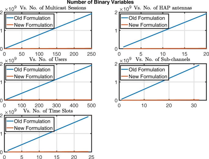

  

  Illustration of the number of binary variables versus the different problem dimensions for (OP1) in [24] (old formulation) and ${\mathcal {H}\mathcal {A}\mathcal {P}}^{Eff}_{MBQCP}$ (new formulation)

  Fig. 7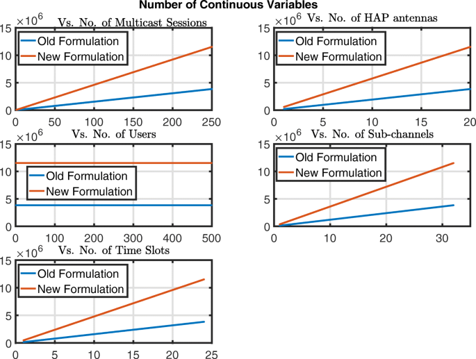

  

  Illustration of the number of continuous variables versus the different problem dimensions for (OP1) in [24] (old formulation) and ${\mathcal {H}\mathcal {A}\mathcal {P}}^{Eff}_{MBQCP}$ (new formulation)

  Fig. 8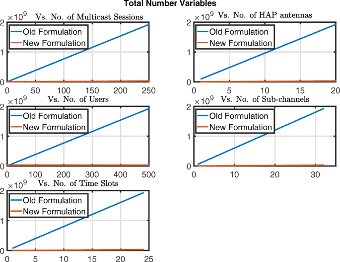

  

  Illustration of the total number of variables versus the different problem dimensions for (OP1) in [24] (old formulation) and ${\mathcal {H}\mathcal {A}\mathcal {P}}^{Eff}_{MBQCP}$ (new formulation)

  Fig. 9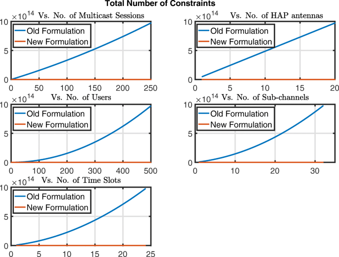

  

  Illustration of the total number of constraints versus the different problem dimensions for (OP1) in [24] (old formulation) and ${\mathcal {H}\mathcal {A}\mathcal {P}}^{Eff}_{MBQCP}$ (new formulation)

  Fig. 10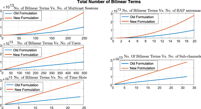

  

  Illustration of the total number of bilinear terms versus the different problem dimensions for (OP1) in [24] (old formulation) and ${\mathcal {H}\mathcal {A}\mathcal {P}}^{Eff}_{MBQCP}$ (new formulation)

• the number of antennas on-board S is varied in the range 1−20.

• the number of users K in the service area is varied in the range 1−500.

• the number of available sub-channels C is varied in the range 1−32.

• the number of available sub-channels T is varied in the range 1−24.

Figures 6, 7, 8, 9 and 10 are comprised of five plots each in which one dimension is varied within its ranges mentioned above and the others are kept fixed at values equal to their maximums in their respective ranges. The results in Fig. 6 show that the number of binary variables for ${\mathcal {H}\mathcal {A}\mathcal {P}}^{Eff}_{MBQCP}$ is way lower than those in (OP1) in [24]. On the other hand in Fig. 7, the number of continuous variables ${\mathcal {H}\mathcal {A}\mathcal {P}}^{Eff}_{MBQCP}$ are almost 4 times those of (OP1) in [24] for the worst case. However by looking at both Figs. 6 and 7, we can see that the number of continuous variables in both formulations are much lower than the binary variables which makes the total number of variables in Fig. 8 almost equivalent to the total number of binary variables. Moreover, it is well known that when there are both binary variables and continuous variables in a problem, the binary variables are the main cause of algorithmic complexity involved in solving the problem. Therefore, comparing the numbers of continuous and binary variables in both formulations, we see that ${\mathcal {H}\mathcal {A}\mathcal {P}}^{Eff}_{MBQCP}$ has a much lower complexity compared to (OP1) in [24].

Taking a look at the number of total constraints in Fig. 9, we see that the number of constraints in formulation ${\mathcal {H}\mathcal {A}\mathcal {P}}^{Eff}_{MBQCP}$ is far lower than (OP1) in [24]. This comes at the cost of up to three times larger number of bilinear terms, in the worst case, for ${\mathcal {H}\mathcal {A}\mathcal {P}}^{Eff}_{MBQCP}$ in all dimensions as Fig. 10 shows. Notice the similar behaviors for both ${\mathcal {H}\mathcal {A}\mathcal {P}}^{Eff}_{MBQCP}$ and (OP1) in [24] in Fig. 10 for each dimension. For the dimensions of the number of multicast sessions, m, and the number of HAP antenna onboard, i, the number of bilinear for both formulations grow quadratically. For the other three dimensions, the growth is linear.

8 Proposed solution method: branching schemes and a presolving linearization-based reformulation

This section explains how formulation ${\mathcal {H}\mathcal {A}\mathcal {P}}^{Eff}_{MBQCP}$ is solved. An approach similar to those in [32] and [27] is used in which, an outer approximation is generated by linear underestimation of the non-convex quadratic constraints to relax the problem’s feasible region. The problem becomes a mixed binary linear program (MBLP) and hence an LP solver can be used in a branch and cut algorithm to solve ${\mathcal {H}\mathcal {A}\mathcal {P}}^{Eff}_{MBQCP}$.The branch-and-bound (BnB) algorithm recursively splits the problem into smaller subproblems, thereby creating a branching tree and implicitly enumerating all potential solutions. At each subproblem, domain propagation is performed to exclude further values from the variables’ domains, and a relaxation may be solved to achieve an upper (dual) bound. The relaxation is then strengthened by adding further valid constraints, which cut off the optimum of the relaxation. Primal heuristics are integrated in the BnB procedure to improve the lower (primal) bound. The solver used for the experiments is Solving Constraint Integer Programs (SCIP) which is capable of solving a non-convex mixed integer quadratically constraint program (MIQCP) to optimality in finite time [33]. The interdependencies between the algorithmic components of SCIP solver are shown in Fig. 11. An explanation for the components used in the experiments done for ${\mathcal {H}\mathcal {A}\mathcal {P}}^{Eff}_{MBQCP}$ are provided in this section and Section 8. The components are the following:

• Presolving

  Fig. 11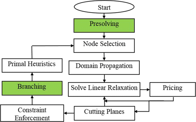

  

  Flowchart illustrating the interrelation between the SCIP solver components used for solving the HAP multicasting AC-RRA problem

• Branching

• Separating cuts

• Domain propagation

• Primal heuristics

The two components considered in this section are the green colored boxes in Fig. 11, which are presolving and branching.

8.1 Presolving reformulation linearization for a particular quadratic constraint set ${\mathcal {H}\mathcal {A}\mathcal {P}}^{Eff}_{MBQCP}$

Presolving is a set of operations invoked before the branch-and-bound algorithm to transform the problem instance to an easier instance to solve. In this section, for the presolving phase for ${\mathcal {H}\mathcal {A}\mathcal {P}}^{Eff}_{MBQCP}$, we consider one of the reformulations in [32] which is a linear reformulation for bilinear terms that are a product of a binary variable $\ddot {x}$ with a linear term, i.e., $\ddot {x}\sum _{j=1}^{k}a_{i}\ddot {y}$. This type of reformulation is applicable to the constraint set $\overline {C8}$ in ${\mathcal {H}\mathcal {A}\mathcal {P}}^{Eff}_{MBQCP}$ where the terms that consist of the product of binary variables and linear terms are $y_{m,i,c,t}\sum _{m=1}^{M}\sum _{i=1}^{S}g_{i^{\prime },k,c,t}p_{m,i^{\prime },c,t}$. The product is replaced by the auxiliary variable z and the linear constraints:

$$ \tilde{p}^{L}y_{m,i,c,t} \leq z \leq \tilde{p}^{U}y_{m,i,c,t}, $$

(38a)

$$ {\begin{aligned} \sum_{m=1}^{M}\sum_{\forall i^{\prime}\neq i}^{}g_{i^{\prime},k,c,t}p_{m,i,c,t}&-\tilde{p}^{L}\left(1-y_{m,i,c,t}\right)\leq z \leq \sum_{m=1}^{M}\sum_{\forall i^{\prime}\neq i}^{}g_{i^{\prime},k,c,t}p_{m,i,c,t}\\ &~~~~~~~~~~~~~~~~~~~~~~~~~~~~~~~~~~~~~~~~~-\tilde{p}^{U}\left(1-y_{m,i,c,t}\right), \end{aligned}} $$

(38b)

where

$$ \tilde{p}^{L}=\sum_{m=1}^{M}\sum_{\forall i^{\prime}\neq i}^{}g_{i^{\prime},k,c,t}\tilde{p}^{L}_{m,i,c,t}, $$

(39a)

$$ \tilde{p}^{U}=\sum_{m=1}^{M}\sum_{\forall i^{\prime}\neq i}^{}g_{i^{\prime},k,c,t}\tilde{p}^{U}_{m,i,c,t}, $$

(39b)

given the local bounds $\tilde {p}^{L}_{m,i,c,t}$ and $\tilde {p}^{U}_{m,i,c,t}$. This reformulation linearizes the constraint set $\overline {C8}$ at the expense of introducing one continuous variable for each constraint in the set, and four linear constraints for each quadratic constraint in $\overline {C8}$. In Section 8.4, the algorithmic performance criteria, with and without, the presolving linearization reformulation explained in this section, for different number of presolving rounds, are presented.

After the presolving phase, the BnB algorithm is invoked. Any reference for ${\mathcal {H}\mathcal {A}\mathcal {P}}^{Eff}_{MBQCP}$ in the rest of this section refers to the instance after going through the presolving phase.

8.2 Branch and bound-based solution framework

The branch and bound scheme is a general framework used in solving non-convex problems, which include MBLPs and MBQLPs, to divide it into smaller problems that can be solved (conquered) and hence is a divide and conquer algorithm [34]. The best local solution across all the subproblems, which are referred to as nodes, is the global solution of the entire problem. Branching is basically the splitting of a subproblem into two or more nodes. Since the discrete variables that we have in ${\mathcal {H}\mathcal {A}\mathcal {P}}^{Eff}_{MBQCP}$ are binary by nature, binary branching is the only choice, i.e., no more than two children nodes for any node in the tree. The root node is the whole problem ${\mathcal {H}\mathcal {A}\mathcal {P}}^{Eff}_{MBQCP}$ before division while the rest of the nodes are smaller subproblems that have either been solved or still need to be solved.

The bounding step avoids complete enumeration of potential solutions of the problem. The better the dual $\ddot {c}_{dual}$ and primal $\ddot {c}_{primal}$ bounds are, the more effective the bounding process in excluding subproblems from solving. The dual bound is found by solving the relaxation $\mathcal {Q}_{relax}$ of a node subproblem $\mathcal {Q}$. The relaxation $\mathcal {Q}_{relax}$ for ${\mathcal {H}\mathcal {A}\mathcal {P}}^{Eff}_{MBQCP}$ is obtained by replacing all the bilinear terms individually by McCormick linear underestimators [32], and by relaxing all the binary variables into the continuous domain [0,1]. Algorithm 1 illustrates the main procedures of a BnB framework. To simplify the notation in the rest of our discussion, and wherever specific reference to certain variables in our formulation ${\mathcal {H}\mathcal {A}\mathcal {P}}^{Eff}_{MBQCP}$ is not required, all the decision variables in ${\mathcal {H}\mathcal {A}\mathcal {P}}^{Eff}_{MBQCP}$ are represented by the decision vector $\ddot {\mathbf {x}}$. Furthermore, an arbitrary decision variable is referred to as $\ddot {x}_{j}$, where $j \in \tilde {N}$ for any variable and if the variable is binary then additionally $j \in \mathcal {B}$, where $\tilde {N}$ is the set of all decision variables and $\mathcal {B}$ is the set of all binary decision variables in ${\mathcal {H}\mathcal {A}\mathcal {P}}^{Eff}_{MBQCP}$.

The input to the algorithm is a presolved instance of ${\mathcal {H}\mathcal {A}\mathcal {P}}^{Eff}_{MBQCP}$ which resembles the root node. If the instance is feasible then the output of the algorithm is the global optimal solution $\ddot {\mathbf {x}}^{\mathcal {HAP}^{Eff}_{MBQCP}}_{opt}$ and the corresponding objective function value $\ddot {c}^{\mathcal {HAP}^{Eff}_{MBQCP}}_{opt}$, otherwise the algorithm concludes that the instance is infeasible. The algorithm is initialized by assigning the root node $\mathcal {HAP}^{Eff}_{MBQCP}$ into the empty node queue $\ddot {\mathcal {L}}$. The Abort procedure is invoked when the node queue is empty to return the best feasible solution found so far $\ddot {\mathbf {x}}_{BFS}$ and its corresponding objective function value $\ddot {c}_{primal}$. If the node queue still has further unprocessed nodes the Select procedure is invoked to choose a node $\mathcal {Q}$ depending on a node selection criterion before it gets removed from the queue. The relaxation of the selected node $\mathcal {Q}_{relax}$ is solved using the simplex algorithm [35] after applying McCormick under-estimators to outer-approximate the non-convex quadratic constraints of ${\mathcal {H}\mathcal {A}\mathcal {P}}^{Eff}_{MBQCP}$. If $\mathcal {Q}_{relax}$ is found infeasible then $\ddot {c}_{dual}$ is assigned the smallest possible value (theoretically −∞) to insure that the node gets pruned in the Bound. Otherwise $\ddot {\mathbf {x}}_{relax}$ becomes the solution of $\mathcal {Q}_{relax}$ and $\ddot {c}_{dual}$ is its corresponding objective function value.

The Bound procedure is responsible for pruning branches from the search tree whose descendant nodes are guaranteed not to include any solutions better than the currently available best feasible solution (incumbent) $\ddot {\mathbf {x}}_{BFS}$. This is known using the simple comparison between the obtained $\ddot {c}_{dual}$ from the Solve procedure and the objective function value $\ddot {c}_{primal}$ for the incumbent. In a maximization problem, like ${\mathcal {H}\mathcal {A}\mathcal {P}}^{Eff}_{MBQCP}$, if the dual (upper) bound is lower than the primal (lower) bound value, this is an indication that any of the descendants of the node can never have any better feasible solutions. If the node gets pruned, the algorithm goes back to the Abort procedure to check if there are any nodes left in the queue $\ddot {\mathcal {L}}$. If no pruning occurs, the Feasibility Check procedure is invoked and sets the solution $\ddot {\mathbf {x}}_{relax}$ of the relaxed subproblem $\mathcal {Q}_{relax}$ as the solution of the $\mathcal {Q}$ itself only if the solution $\ddot {\mathbf {x}}_{relax}$ is feasible to $\mathcal {Q}$. If $\ddot {\mathbf {x}}_{relax}$ is not feasible to $\mathcal {Q}$, the Branch procedure then gets invoked to divide node $\mathcal {Q}$ into further nodes. This happens by selecting an appropriate variable to branch on. Since all the discrete variables in ${\boldsymbol{\mathcal {H}}\boldsymbol{\mathcal {A}}\boldsymbol{\mathcal {P}}}^{Eff}_{MBQCP}$ are binary, then the branching is also binary. After branching takes place, the Abort procedure gets invoked to check whether there are any unprocessed nodes left in $\ddot {\mathcal {L}}$.

The node selection indicated by the Select procedure, the branching rules indicated by Branch and the relaxation whose solution is used in the Bound procedure all have a major impact on how early good feasible solutions can be found and how fast the dual bounds decreases. They all influence the Bound procedure which is expected to prune large parts of the BnB tree. An explanation for different branching rules used in the experiments conducted on ${\mathcal {H}\mathcal {A}\mathcal {P}}^{Eff}_{MBQCP}$ is provided in Section 8.3.

8.3 Branching

Branching is the splitting of a node into two or more nodes by adding new upper and lower bounds on one of the variables which is called the branching variable. By reducing a variables domain, the created children nodes have smaller feasible regions each, which helps reduce the work required to find feasible solutions better than the currently available best feasible solution $\ddot {\mathbf {x}}_{BFS}$.

One advantage of using LP relaxation within BnB is in the branching process. Branching changes the created children subproblems from a parent node $\mathcal {Q}$ by introducing new upper or lower bound to one variable which preserves the dual feasibility of the solution obtained for $\mathcal {Q}_{relax}$. This enables the use of dual simplex using the parent node solution as a warm up start and hence the work done in solving $\mathcal {Q}_{relax}$ counts towards solving the relaxation of its children, which saves a lot of further computational work.

For ${\mathcal {H}\mathcal {A}\mathcal {P}}^{Eff}_{MBQCP}$, the only discrete variables are binary and hence two nodes only are created by branching on binary variables. A score $s^{branch}_{j}$ is calculated for each variable using the equation [36]:

$$ s^{branch}_{j}=max\left \{ \ddot{q}^{0}_{j}, \overline{\epsilon} \right \}max\left \{ \ddot{q}^{1}_{j}, \overline{\epsilon} \right \}, $$

(40)

which measures the improvement in the dual bound by branching on the variable $\ddot {x}_{j}$ for $j \in \mathcal {B}$ where:

• $\mathcal {B}$ is the set of binary variables in ${\mathcal {H}\mathcal {A}\mathcal {P}}^{Eff}_{MBQCP}$,

• $\ddot {q}^{0}_{j}$ is a function that is directly dependent on and proportional to the dual bound improvement $\ddot {\Delta }^{0}_{j}$ over the parent subproblem’s relaxation $\mathcal {Q}_{relax}$ by setting $\ddot {x}_{j}=0$,

• $\ddot {q}^{1}_{j}$ is a function that is directly dependent on and proportional to the dual bound improvement $\ddot {\Delta }^{1}_{j}$ over the parent subproblem’s relaxation $\mathcal {Q}_{relax}$ by setting $\ddot {x}_{j}=1$,

• $\overline {\epsilon }$ which is a very small positive constant which is necessary to compare $\left (\ddot {\Delta }^{0}_{j},\ddot {\Delta }^{1}_{j}\right)$ and $\left (\ddot {\Delta }^{0}_{k},\ddot {\Delta }^{1}_{k}\right)$ and is set by default to $\overline {\epsilon } =10^{-6}$ in SCIP.

There many different ways by which a branching variable can be selected, and of course, they can have different performances in bound improvement which are illustrated in the results provided in Section 8.4. The following branching schemes are considered for ${\mathcal {H}\mathcal {A}\mathcal {P}}^{Eff}_{MBQCP}$ [28, 36].

8.3.1 Random branching

As the name indicates, there is nothing done in this technique except arbitrarily selecting any unfixed binary variable that violates the binary condition.

8.3.2 Most infeasible branching

This rule chooses the variable with the smallest tendency to be rounded either downwards or upwards. Hence for binary variables with fractional values in the solution of $\mathcal {Q}_{relax}$, the one that is closest to 0.5 receives the highest score. The score function for a fractional binary variable is given as:

$$ s^{branch}_{j}=min\left \{ \ddot{x}_{j}^{relax},1-\ddot{x}_{j}^{relax}\right \},~~j \in \mathcal{B}. $$

(41)

8.3.3 Pseudocost branching

This type of branching keeps a history for the average performance of each variable that has been branched on so far. This is measured as the average improvement in the bound for all the times the variable has been branched on. To obtain the variable scores, first the unit bound change for $\ddot {x}_{j}$ is found using

$$ \varsigma^{0}_{j}=\frac{\ddot{\Delta}^{0}}{\ddot{x}_{j}^{relax}} \qquad and \qquad \varsigma^{1}_{j}=\frac{\ddot{\Delta}^{1}}{\left(1-\ddot{x}_{j}^{relax}\right)}. $$

(42)

Let the aggregate unit bound changes be $\ddot {\sigma }^{0}_{j}$ and $\ddot {\sigma }^{1}_{j}$ over all nodes for which $\ddot {x}_{j}$ was selected for branching and the numbers of these nodes be $\eta ^{0}_{j}$ and $\eta ^{1}_{j}$ then the pseudocosts of $\ddot {x}^{j}$ are the averages:

$$ \Psi^{0}_{j} =\frac{\ddot{\sigma}^{0}_{j}}{\eta^{0}_{j}} \qquad and \qquad \Psi^{1}_{j} =\frac{\ddot{\sigma}^{1}_{j}}{\eta^{1}_{j}}. $$

(43)

The score is then given as:

$$ {\begin{aligned} s^{branch}_{j}=max\left \{ \ddot{x}^{j}_{relax} \Psi^{0}_{j},\overline{\epsilon} \right \}.max\left \{\left(1-\ddot{x}^{j}_{relax}\right)\Psi^{1}_{j}, \overline{\epsilon} \right \}. \end{aligned}} $$

(44)

During the course of Algorithm 1, a variable that has not yet been selected for branching is termed to be uninitialized, a term that will be used in subsequent subsections.

8.3.4 Strong branching

Strong branching can be summarized as solving the linear relaxations that result from branching on each binary branching candidate and choosing the variable that gives the best bound improvement to branch on. It is hence expected that to obtain the optimal solution for a problem instance, the number of nodes required to be explored is going to be low but the number of simplex LP iterations is going to be too high which consumes a lot of processing time. The full set of branching candidates F_cand are all binary variables with fractional values. The entire set could be used in strong branching or only a subset $\overline {\mathit {F}} \subset \mathit {F}_{cand}$.

8.3.5 Hybrid strong/pseudocost branching

Strong branching and pseudocost branching both have their advantages and draw backs. For strong branching, as mentioned in Section 8.3.4, the number of nodes to be explored before the optimal solution is reached is expected to be low. However, the time and LP iterations expended could be too high. On the other hand, pseudocost branching is not expected to expend too many LP iterations (and hence time) to obtain the optimal solution, but would require more branching operations to do so and hence more number of nodes. This is because at the very beginning of the BnB tree, the pseudocost branching scheme has no history to use for guiding its choice on branching. Since the branching decisions near the top of the BnB tree are the most crucial, the absence of early history information would lead to more node explorations. If the optimal solution is not the main objective and obtaining solutions with low duality gap is desired in a given time, it is expected that strong branching would return a large duality gap since the rate of improvement is expected to be slow for the given solution time due to the high number of LP iterations required. A hybrid branching technique, that combines both schemes, aims to get the best of each and reduce as much as possible the cons each has. It is achieved by implementing strong branching in the upper part of BnB tree up to a certain depth d. For nodes that are deeper than d in the tree, pseudocost branching is applied.

8.3.6 Reliability branching

The branching decision based on pseudocosts either in pure pseudocost branching or in hybrid strong/pseudocost branching are based on uninitialized values which negatively affect the selection of branching variables. Reliability branching uses strong branching for variables with uninitialized pseudocosts (defined in Section 8.3.3), and hence is more dynamic than hybrid strong/pseudocost branching which uses strong branching for a fixed depth in the BnB tree. Furthermore, to use the pseudocosts for branching, reliability branching requires that the history for the branching variable be collected for at least η_rel problems, where η_rel is the reliability parameter. Hence if $min\left \{ \eta ^{0}_{j}, \eta ^{1}_{j} \right \} \leq \eta _{rel}$ the variable $\ddot {x}_{j}$ is called unreliable. Moreover, the work expended in strong branching can be reduced by using a small subset of branching variable candidates $\overline {\mathit {F}} \subset {F}_{cand}$ as well as performing only a few simplex iterations for each candidate in $\overline {F}$ to estimate the changes in the dual bound. The dual bound is the value of the objective function of $\mathcal {Q}_{relax}$. Since the change in the objective function value is greatest in the first few simplex iterations compared to later iterations, the estimate for the dual bound is expected to be close to the actual value.

The η_rel dynamically changes to restrict the number of strong branching simplex iterations for a given node $\mathcal {Q}$ to [37] :

$$ \hat{\gamma}^{max}_{SB}=c_{sbiterquot} \hat{\gamma}_{LP}+ \hat{\gamma}^{root}_{SB}+\hat{\gamma}_{fixed}, $$

(45)

where

• $\hat {\gamma }^{max}_{SB}$ is the number of simplex iterations for the strong branching done in $\mathcal {Q}$

• $\hat {\gamma }_{LP}$ is the number of regular simplex iterations

• c_sbiterquot is maximal fraction of strong branching LP iterations compared to node relaxation LP iterations,

• $\hat {\gamma }_{fixed}$ is a fixed number that can be pre-set.

If the number of strong branching LP iterations $\hat {\gamma }_{SB}$ exceeds $\hat {\gamma }^{max}_{SB}$, then η_rel is set to zero and pseudocost branching is used. If $\hat {\gamma }_{SB} \in \left [ c_{sbiterquot}\hat {\gamma }^{max}_{SB},\hat {\gamma }^{max}_{SB} \right ]$, η_rel decreases from $\eta ^{max}_{rel}$ to $\eta ^{min}_{rel}$ linearly. If $\hat {\gamma }_{SB}< c_{sbiterquot}\gamma _{LP}$, then η_rel increases in proportion to the quotient $\frac {\hat {\gamma }_{LP}}{\hat {\gamma }^{max}_{SB}}$.

8.3.7 Inference branching

This technique exploits domain propagation of branching variables. Its main idea is that it selects the variable whose domain tightening (variable fixation in case of binary variables) produces the most domain reductions in other variables. The impact of a variable on domain deductions is obtained from history information, like pseudocost branching, that measures the average inferred domain deductions $\ddot {\Phi }^{1}_{j}$ and $\ddot {\Phi }^{0}_{j}$ given by [36]:

$$ \ddot{\Phi}^{1}_{j}=\frac{\ddot{\phi}^{1}_{j}}{\ddot{\nu^{1}_{j}}} \qquad and \qquad \ddot{\Phi}^{0}_{j}=\frac{\ddot{\phi}^{0}_{j}}{\ddot{\nu^{0}_{j}}}, $$

(46)

where

• $\ddot {\Phi }^{1}_{j}$ and $\ddot {\Phi }^{0}_{j}$ are the total deductions by setting the binary variable $\ddot {x}_{j}$ to 1 or 0 respectively,

• $\ddot {\nu ^{1}_{j}}$ and $\ddot {\nu ^{0}_{j}}$ are the numbers of corresponding subproblems for which domain propagation has been applied.

For uninitialized binary variables, clique and implication tables are used to calculate the inference values [36].

8.3.8 Cloud branching

All branching strategies described above deal with only one optimal fractional solution for $\mathcal {Q}_{relax}$. Whereas LP relaxations are known to be largely degenerate, multiple equivalent optimal solutions are the rule rather than the exception. Therefore considering only one optimal solution yields high possibilities of taking arbitrary, or inefficient branching decisions. Cloud branching exploits the knowledge of a cloud of multiple alternative optimal solutions of the given LP relaxation using dual degeneracy in a mixed integer program [38]. For a given cloud of optimal solutions of the LP relaxation, the initial set of branching variable candidates contains all the variables that are fractional in at least one solution of the cloud . The cloud of solutions is generated in the context of strong branching which solves the LPs that would result from branching on all candidates.

The first step in the cloud branching strategy is to generate a cloud of alternative optimal solutions for the LP relaxation $\mathcal {Q}_{relax}$ of a node $\mathcal {Q}$. This is done by restricting search for the basic feasible variables to the optimal hyperplane of the polyhedron. To implement this type of search, the variables of a given optimal solution, whose reduced costs are non-zero need to be fixed in the search procedure. To move from one basis to another on the optimal hyperplane, an auxiliary objective function is needed. The one used in our numerical experiments is a feasibility like pump objective function that is implemented in the SCIP solver and was proposed in [38] whose coefficients for the binary variables $j \in \mathcal {B}$ are given as:

$$ c_{j}= \left\{\begin{array}{lll} -1~~if ~0<\ddot{x}^{*}_{j} <0.5 \\ 1~~if ~0.5 \leq \ddot{x}^{*}_{j}<1. \end{array}\right. $$

(47)

Using iterations of the primal simplex algorithm on the resulting auxiliary LP $\mathcal {Q}_{Aux}$, an alternative optimum basis to the LP relaxation of the BnB node can be obtained that has the closest hamming distance to the nearest integral point.

After obtaining a cloud , the cloud interval for a variable is given by , where:

(48a)

(48b)

Accordingly, the set is partitioned into three which are:

(49a)

(49b)

(49c)

which shows that for binary variables, the only type of discrete variables in ${\mathcal {H}\mathcal {A}\mathcal {P}}^{Eff}_{MBQCP}$, F₂ contains the fractional variables of all the solutions in the cloud .

Branching on the variables in F₀ guarantees that the dual bound in both branching directions will not improve. Those in F₁ are guaranteed not to improve the bound in only one direction but hopefully will improve in the other direction. The candidates in F₂ are expected to improve the dual bound in both directions. The cloud purpose is to filter out as many LPs so that strong branching only needs to solve a small subset of those. As long as there are any candidates existing in the set F₂, the other two sets are ignored and only the LPs for the candidates in F₂ are solved.

8.4 Computational experiments, results, and discussions

This section discusses the experiments conducted for ${\mathcal {H}\mathcal {A}\mathcal {P}}^{Eff}_{MBQCP}$ and presents the numerical results obtained for the algorithmic procedures given in Sections 8.1 and 8.3 to evaluate their performances. Two different experiment sets are provided in this section. The first experiment set (Section 8.5) compares the performance of activating-versus-deactivating the reformulation linearizion technique, at the presolving phase, for the quadratic constraint set $\overline {C8}$ in ${\mathcal {H}\mathcal {A}\mathcal {P}}^{Eff}_{MBQCP}$ which was explained in Section 8.1. The second experiment set (Section 8.6) compares the performance of the different branching techniques explained in Section 8.3. The performance for each set of experiments is measured using the following criteria:

• 1. The duality gap

• 2. Number of LP iterations expended

• 3. Number of nodes in the search tree

• 4. Average number of LP iterations per node

The experiments were performed in Matlab, for which the open source optimization toolbox OPTI (version 2.16) [39] provided the interface with the SCIP 3.2.0 solver [33]. SCIP 3.2.0 is the solver used in all the experiments conducted for ${\mathcal {H}\mathcal {A}\mathcal {P}}^{Eff}_{MBQCP}$. The experiments were performed on a machine with a 6 core 3.5 GHz Intel Xeon processor. Using the parallel processing toolbox in Matlab, we were able to conduct different experiments in parallel. For example, to conduct experiments on different branching strategies, each CPU core performed the experiment of a specific branching strategy for the same set of problem instances in parallel. The generic SCIP solver settings used in all the experiment sets performed are given in Table 2.

Table 2 Generic SCIP solver settings for all experiment sets conducted

One hundred instances were solved for each experiment. Each instance has a size of 527 variables and 4261 constraints out of which 107 variables are binary and 2844 constraints are quadratic. To obtain the channel gain g_i,k,c,t values, a simulation was conducted using the parameters in Table 3, Eq. (4) in this paper and (13), (14) and (15) from our earlier work in [24]. The channel consists of a free space pathloss propagation model, Ricean fading as suggested in [1], the rain attenuation model in [29], the HAP aperture antenna model in [21] and parabolic reflector user antennas. In the simulation, the user positions change during every iteration according to a uniform probability distribution about the HAP footprint centers. The degree of overlap between antenna footprints is defined as the ratio between the overlap distance d_overlap, illustrated in Fig. 12, and the HAP antenna footprint radius r_footprint. Figure 3 in Section 1 illustrates the overlapped HAP antenna footprints in our experiments.

Fig. 12

Two overlapping antenna beam footprints

Table 3 Simulation parameters for HAP multicasting environment

To evaluate the average performance of all the instances for each experiment, arithmetic, geometric and shifted geometric means were used. For the shifted geometric mean, the shifting parameters values used are the following:

• 1. 50, for the dual gap

• 2. 100, for the number of BnB nodes

• 3. 1000, for the number of LP iterations

The shifted geometric mean of a sample ω₁,ω₂,...,ω_k is given in[36]:

$$ \psi_{s}=\left(\prod_{j=1}^{k}max\left \{ \omega_{j} +s,1\right \}\right)^{1/k}-s, $$

(50)

where s is the shifting parameter. For geometric mean, s=0. In the comments made on the results in the following subsections, we use the shifted geometric means for comparison except for the average number of LP iterations per node which uses only arithmetic means.

The duality gap is calculated in all the experiments, in percentage, using the formula:

$$ \varrho = \frac{\left | \ddot{c}_{dual}-\ddot{c}_{primal} \right |} {min\left(\left|\ddot{c}_{dual}\right|,\left|\ddot{c}_{primal}\right|\right) }. $$

(51)

8.5 Computational experiments and results: reformulation linearization at presolving phase

In this sub-section, the experimental procedures and results for the reformulation linearization technique explained in Section 8.1 are provided. The reformulation technique is invoked at the presolving phase and hence the experiments illustrate the performance of activating-versus-deactivating the linearization for the number of presolving rounds 1, 5, 25, 50 and 100. The following settings were considered for the reformulation linearization experiments:

• 1. Node selection scheme is best first search with a maximum plunging depth in the BnB tree of 2 [33],

• 2. Most infeasible branching scheme was used and

• 3. The only heuristic used was the Undercover heuristic [40].

In Figs. 13, 14, 15, and 16 the duality gap, the number of LP iterations, the number of BnB nodes and the average number of LP iterations per node are illustrated for the reformulation linearization experiments. In those figures, RndNumi:‘.’, indicates the number of presolving rounds is i for either: “A,” activated reformulation linearization or “D,” deactivated reformulation linearization.

Fig. 13

Reformulation linearization results: duality gap

Fig. 14

Reformulation linearization results: number of LP iterations

Fig. 15

Reformulation linearization results: number of BnB nodes

Fig. 16

Reformulation linearization results: average number of LP iterations per node

We can see that for a single presolving round, the dual gap is almost the same in both “A” and “D.” The number of BnB nodes is slightly lower by around 11% for “A” compared to “D.” The number of LP iterations and the average number of LP iterations per node are almost equal for “A” and “D.”

A small increase in the number of presolving rounds to 5 yields an increase in the dual gap for both cases “A” and “D” as shown in Fig. 13. However, the dual gap for “D” is lower than that of “A” by around 30% at the expense of a much larger number of nodes in comparison to “A” (more than 2700%). The number of explored nodes is lower for both “A” and “D” for five presolving rounds as compared to one presolving round as Fig. 15 shows. For “A,” it is lower by around 99% and “D” is lower by 50%. The number of LP iterations decreases by around 85% for “A” and increases by 15% for “D” making it higher than “A” by almost 800%. According to Fig. 16, the number of average LP iterations expended per node for five presolving rounds is around 2500% higher for “A” compared to “D.” Comparing five presolving rounds versus one, the average number of LP iterations per node increased by 5100% for “A” but only by 100% for “D.”

Increasing the number of presolving rounds from 5 to 25 shows that the duality gap reduces for both ‘A’ and ‘D’ by 29% and 31% respectively (almost same reduction), while “D” still has a lower dual gap by 30% compared to ‘A’. The reduction in dual gap achieved by increasing the number of presolving rounds from 5 to 25, is accompanied by a reduction in the number of nodes in “D” by about 31% and a very small increase in the number of nodes in “A.” For 25 presolving rounds, the number of LP iterations for “A” is lower than “D” by about 65% but the number of average LP iterations per node is much higher by about 2450%.

For presolving rounds 25, 50 and 100, it can be seen in Fig. 13 that ‘D’ maintains the same duality gap while that of “A” keeps decreasing. For 100 presolving rounds, we can see that “A” has a duality gap lower than “D” by 60%. The number of BnB nodes gradually decreases slightly for “D” when increasing the presolving rounds in the range 25, 50, and 100 while that for “A” keeps increasing such that the number of nodes for 100 rounds increases by about 900%. However at 100 presolving rounds, the number of nodes for “A” is lower than “D” by about 70%. Figure 14 shows that the number of LP iterations for presolving rounds 25, 50, and 100 remains approximately the same for “D” but increases slightly for “A.” For presolving rounds 5, 25, 50, and 100, it can be seen from Fig. 16 that the average number of LP iterations per node decreases enormously versus the number of rounds for “A” and becomes equivalent to “D” whose average LP iterations per node remains the same for rounds 5, 25, 50, and 100.

From the results, we can hence conclude that it is beneficial to use the reformulation linearizion technique for constraint set $\overline {C8}$ with a high number of presolving rounds (around 100).

8.6 Computational experiments and results: branching schemes

In this section, the experimental procedures and results for the branching techniques given in Section 8.3 are provided. Strong Branching is not considered by itself in the experiments due to its expected high computational effort and time. However as explained in Section 8.3, it is a component of hybrid strong/psedocost, reliability and cloud branching where its effect will be seen in those branching schemes. The following settings are considered for the experiments conducted for the branching schemes:

• 1. Separating cuts are deactivated.

• 2. Node selection scheme is best first search with a maximum plunging depth in the BnB tree of 2 [33].

• 3. Up to one round of presolving before starting the BnB algorithm.

• 4. For hybrid strong/pseudocost branching, maximum strong branching depths of $\tilde {d}_{strong}=1$ and $\tilde {d}_{strong}=2$ are tried in two different experiments.

• 5. For reliability branching the following settings are considered:

  • The maximum value for the reliability threshold is $\eta ^{max}_{rel}=5$,

  • the minimum value for the reliability threshold is $\eta ^{min}_{rel}=1$,

  • $\hat {\gamma }_{fixed}=0$ in Equation (5.8) in [28],

  • maximum size of the set of strong branching candidates, $\overline {\mathit {F}} =15$,

  • maximum number of strong branching simplex iterations per branching variable is $\hat {\gamma }_{sbiterbrancand}=100$,

  • the ratio c_sbiterquot in Equation (5.8) in [28] is set to c_sbiterquot=0.05 and c_sbiterquot=0.2 for two different experiments.

Figures 17, 18, 19, and 20 show the duality gap, number of LP iterations, number of BnB nodes and the average number of LP iterations per node for the different branching schemes. In those figures, HybDepth1 and HybDepth2 are the hybrid strong/pseudocost branching with strong branching invoked up to maximum depths of 1 and 2 respectively. Furthermore, Relratio=0.05 and Relratio=0.2 refer to reliability branching with c_sbiterquot=0.05 and c_sbiterquot=0.2. It can be seen that random branching has the highest duality gap, which is expected since the selection of branching candidates does not take into account the direction of change of the dual bound. The lowest duality gap was achieved (almost equally) by inference branching, pseudocost branching, hybrid strong/pseudocost branching ($\tilde {d}_{strong}=1$), and surprisingly most infeasible branching. The second lowest are the cloud branching and reliability branching with c_sbiterquot=0.05 equally both having a higher duality gap than the lowest four by about 18%. Finally the second highest duality gap is obtained by reliability branching with c_sbiterquot=0.2 with a duality gap higher than the lowest four by 50%.

Fig. 17

Branching results: duality gap

Fig. 18

Branching results: number of LP iterations

Fig. 19

Branching results: number of BnB nodes

Fig. 20

Branching results: average number of LP iterations per node

Comparing pseudocost branching versus hybrid strong/pseudocost branching with $\tilde {d}_{strong}=1$, it can be seen that they almost perform equally in terms of duality gap, number of expended LP iterations, number of nodes and the average LP iterations per node. Increasing the depth for strong branching to $\tilde {d}_{strong}=2$ in hybrid strong/pseudocost branching leads to an increase in the duality gap by 32%. This is because when more strong branching is involved, a slightly greater number of LP iterations per node are expended as shown in Fig. 20, meaning that in a given time limit, fewer nodes are explored as shown in Fig. 19. When fewer nodes are explored for a given time limit, the overall dual bound improvement could be lower, even though the improvement per node can be higher for strong branching. The same reasoning applies for reliability branching in the two experiments in which c_sbiterquot=0.05 and c_sbiterquot=0.2.

Among the four branching schemes that give the lowest duality gaps, inference branching needs the largest number of nodes and LP iterations as Figs. 18 and 19 show. Cloud branching expends the lowest number of nodes and LP iterations among all the branching schemes but has the second lowest duality gap. It requires 64% less number of nodes and 58% less number of LP iterations compared to most infeasible branching. Although cloud branching is based on strong branching, the cloud reduces out many LPs so that strong branching solves a small subset of those. It hence gives a better duality gap than HybDepth2 and reliability branching at c_sbiterquot=0.2 requiring lower number of BnB nodes and LP iterations. It also gives an equally good duality gap for lower number of BnB nodes and LP iterations compared to reliability branching with c_sbiterquot=0.05.

According to the observations and analysis based on the results in Figs. 17, 18, 19, and 20, cloud branching seems to have a good trade-off balance of all the criteria of interest.

9 Conclusions

In this paper, we extended a problem in our earlier works and we were successful in obtaining a more efficient formulation. For the problem considered in this paper, a user was allowed to join any session being transmitted in all the neighboring cells provided the SINR threshold was met where as P-Prob, the problem we considered in our earlier works, a user only can join a subset of the sessions being transmitted in the one cell which is the one the user resides in. Moreover, E-Prob allowed a multicast group to receive transmission of a session on more than one antenna simultaneously, which is a more flexible proposal that utilizes the space dimension, that was not utilized in the primary problem. Also, the extended problem took into account heterogeneous user and session priorities which were considered to be homogeneous in P-Prob. We were successful in obtaining ${\mathcal {H}\mathcal {A}\mathcal {P}}^{Eff}_{MBQCP}$, a formulation that is far more efficient in terms of the size compared to formulation (OP1) in [24], the formulation used for P-Prob. The more efficient formulation ${\mathcal {H}\mathcal {A}\mathcal {P}}^{Eff}_{MBQCP}$ was a separate achievement on its own that was used in E-Prob. In other words, if E-Prob was reduced to P-Prob, ${\mathcal {H}\mathcal {A}\mathcal {P}}^{Eff}_{MBQCP}$ would still be much more efficient than (OP1) in [24].

We used a BnB based solution framework proposed for solving ${\mathcal {H}\mathcal {A}\mathcal {P}}^{Eff}_{MBQCP}$. Two aspects of the solution framework were considered, a presolving reformulation linearization for a particular set of quadratic constraints in the formulation and a number of different branching schemes. For the presolving reformulation linearization, the aim was to find whether it would make the solution procedure more efficient and to evaluate the tradeoffs. According to the results obtained from the experiments that we conducted, we found that reformulation linearization is recommended when applying at least 100 presolving rounds as this gave the lowest duality gap as well as low number of LP iterations and nodes as compared not applying the reformulation linearization technique. For the branching schemes, we showed that cloud branching has a good tradeoff between the duality gap, number of LP iterations and number of BnB nodes when compared with the other branching schemes.

Finally, it is worth noting that the complexity analysis of the proposed algorithm is a challenging problem which deserves to be investigated as a future research work.

References

E. Falletti, M. Laddomada, M. Mondin, F. Sellone, Integrated services from high-altitude platforms: a flexible communication system. IEEE Commun. Mag.44(2), 85–94 (2006).
G. M. Djuknic, J. Freidenfelds, Y. Okunev, Establishing wireless communications services via high-altitude aeronautical platforms: a concept whose time has come?IEEE Commun. Mag.35(9), 128–135 (1997).
A. Mohammed, A. Mehmood, F. Pavlidou, M. Mohorcic, The role of high-altitude platforms (HAPs) in the global wireless connectivity. Proc. IEEE. 99(11), 1939–1953 (2011).
P. Sudheesh, M. Mozaffari, M. Magarini, W. Saad, P. Muthuchidambaranathan, Sum-rate analysis for high altitude platform (hap) drones with tethered balloon relay. IEEE Commun. Lett.22(6) (2018).
D. Xu, X. Yi, Z. Chen, C. Li, C. Zhang, B Xia, in Personal, Indoor, and Mobile Radio Communications (PIMRC), 2017 IEEE 28th Annual International Symposium on. Coverage ratio optimization for hap communications (IEEEMontreal, 2017), pp. 1–5.
F. Dong, H. Han, X. Gong, J. Wang, H. Li, A constellation design methodology based on qos and user demand in high-altitude platform broadband networks. IEEE Trans. Multimedia. 18(12), 2384–2397 (2016).
J. Zhang, Y. Zeng, R Zhang, in Communications (ICC), 2017 IEEE International Conference on. Spectrum and energy efficiency maximization in UAV-enabled mobile relaying (IEEEParis, 2017), pp. 1–6.
M. Stoneback, K. Madsen, in 2018 IEEE/MTT-S International Microwave Symposium - IMS. A planar all-silicon 256-element ka-band phased array for high-altitude platforms (HAPs) application (IEEE Philadelphia, 2018), pp. 783–786.
W. Theunissen, V. Jain, G. Menon, in 2018 IEEE/MTT-S International Microwave Symposium - IMS. Development of a receive phased array antenna for high altitude platform stations using integrated beamformer modules (IEEEPhiladelphia, 2018), pp. 779–782.
X. Cao, P. Yang, M. Alzenad, X. Xi, D. Wu, H. Yanikomeroglu, Airborne communication networks: a survey. IEEE J. Sel. Areas Commun.36:, 1–1 (2018).
X. Liu, M. Jia, Z. Na, W. Lu, F. Li, Multi-modal cooperative spectrum sensing based on Dempster-Shafer fusion in 5G-based cognitive radio. IEEE Access. 6:, 199–208 (2017).
X. Liu, et al., 5G-based green broadband communication system design with simultaneous wireless information and power transfer. Phys. Commun.28:, 130–137 (2018).
X Liu, F Li, Z Na, Optimal resource allocation in simultaneous cooperative spectrum sensing and energy harvesting for multichannel cognitive radio. IEEE Access. 5:, 3801–3812 (2017).
D. Grace, M. Mohorcic, Broadband Communications via High-Altitude Platforms (Wiley, Chichester, 2011).
G. Olmo, T. C. Tozer, D. Grace, The European HeliNet Project. 3rd International Airship Convention and Exhibition, Friedrichshafen (Germany), (2000).
F. Dovis, L. L. Presti, E. Magli, G. Olmo, F. Sellone, in Data Systems in Aerospace, vol. 457. HeliNet: A Network of UAV-HAVE Stratospheric Platforms. System Concepts and Applications to Environmental Surveillance (ESA Publ. Div.Neuilly-sur-Seine, Nordwijk, 2000), p. 551.
D. Grace, M. Mohorcic, M. Oodo, M. Capstick, M. B. Pallavicini, M. Lalovic, in Proceedings of the 14th IST Mobile and Wireless and Communications Summit. CAPANINA-Communications from Aerial Platform Networks Delivering Broadband Information for All (European Association for Signal Processing (EURASIP) Dresden, 2005).
CAPANINA project for the development of broadband communications capability HAPs. http://www.capanina.org. Accessed July 2019.
D. Grace, M. H. Capstick, M. Mohorcic, J. Horwath, M. B. Pallavicini, M. Fitch, Integrating Users into the Wider Broadband Network via High Altitude Platforms. IEEE Wirel. Commun.12(5), 98–105 (2005).
R. v. Nee, R. Prasad, OFDM for Wireless Multimedia Communications (Artech House, Norwood, 2000).
J. Thornton, D. Grace, M. H. Capstick, T. C. Tozer, Optimizing an Array of Antennas for Cellular Coverage from a High Altitude Platform. IEEE Trans. Wirel. Commun.2(3), 484–492 (2003).
A. Ibrahim, A. S Alfa, in IEEE Globecom Workshops (GC Wkshps), 2013. Radio Resource Allocation for Multicast Transmissions over High Altitude Platforms (IEEEAtlanta, 2013), pp. 281–287.
A. Ibrahim, A. S Alfa, in Wireless Telecommunications Symposium (WTS), 2014. Solving Binary and Continuous Knapsack Problems for Radio Resource Allocation over High Altitude Platforms (IEEEWashington, 2014), pp. 1–7.
A. Ibrahim, A. S. Alfa, Using Lagrangian Relaxation for Radio Resource Allocation in High Altitude Platforms. IEEE Trans. Wirel. Commun.14(10), 5823–5835 (2015).
G. P. McCormick, Computability of Global Solutions to Factorable Nonconvex Programs: Part I—Convex Underestimating Problems. Mathematical programming. 10(1), 147–175 (1976).
E. L. Lawler, D. E. Wood, Branch-and-Bound Methods: A Survey. Operations research. 14(4), 699–719 (1966).
T. Berthold, A. M. Gleixner, S. Heinz, S. Vigerske, Analyzing the Computational Impact of MIQCP Solver Components. Numer. Algebra Control Optim.2(4), 739–748 (2012).
A. Ibrahim, Admission control and radio resource allocation for multicasting over high altitude platforms. PhD thesis, University of Manitoba, (Winnipeg, 2016).
D. A. Pearce, D. Grace, Optimum Antenna Configurations for Millimetre-Wave Communications from High-Altitude Platforms. IET Commun.1(3), 359–364 (2007).
J. Lee, S. Leyffer, Mixed Integer Nonlinear Programming (Springer, New York, 2012).
C. Cox, An introduction to LTE: LTE, LTE-advanced, SAE and 4G mobile communications (Wiley, Chichester, 2012).
T. Berthold, S. Heinz, S. Vigerske, Extending a CIP Framework to Solve MIQCPs (Springer, New York, 2012).
T. Achterberg, SCIP: Solving Constraint Integer Programs. Mathematical Programming Computation. 1(1), 1–41 (2009). http://mpc.zib.de/index.php/MPC/article/view/4. Accessed Apr 2016.
S. Burer, A Saxena, in Mixed Integer Nonlinear Programming. The MILP Road to MIQCP (SpringerNew York, 2012), pp. 373–405.
W. L. Winston, M. Venkataramanan, J. B. Goldberg, Introduction to Mathematical Programming, vol. 1 (Thomson/Brooks/Cole, Boston, 2003).
T. Achterberg, Constraint Integer Programming. PhD thesis, Technische Universität Berlin, (Berlin, 2007).
T. Achterberg, Solving Constraint Integer Programs (SCIP) Solver Documentation. http://scip.zib.de/doc/html_devel/branch__relpscost_8c_source.php. Accessed Apr 2016.
T. Berthold, D Salvagnin, in Integration of AI and OR Techniques in Constraint Programming for Combinatorial Optimization Problems. D., Cloud Branching (SpringerNew York, 2013), pp. 28–43.
J. Currie, D. I Wilson, in Foundations of Computer-Aided Process Operations, ed. by N. Sahinidis, J. Pinto. OPTI: Lowering the Barrier Between Open Source Optimizers and the Industrial MATLAB User (ElsevierSavannah, 2012), pp. 8–11.
T. Berthold, A. M. Gleixner, Undercover: A Primal MINLP Heuristic Exploring a Largest sub-MIP. Math Program. 144(1-2), 315–346 (2014).
Acknowledgements
This research is supported in part by a grant from the Natural Sciences and Engineering Research Council (NSERC) of Canada. The material in this paper is based on part of the PhD thesis of the first author, under the supervision of the second author. The authors declares that they have no competing interests.
Funding
This research is supported in part by a grant from the Natural Sciences and Engineering Research Council (NSERC) of Canada.
Author information
Authors and Affiliations
Contributions
AI is the primary author of this work. AI and AA contributed to the conception of the study and performed the system analysis. AI developed the simulation and experimental environment and conducted all the experiments and simulations under the full guidance and detailed supervision of AA. AI wrote the manuscript. AA provided great comments to enhance the paper quality. All authors reviewed and approved the final manuscript.
Ethics declarations
Competing interests
The authors declare that they have no competing interests.
Additional information
Publisher’s Note
Springer Nature remains neutral with regard to jurisdictional claims in published maps and institutional affiliations.
Rights and permissions
Open Access This article is distributed under the terms of the Creative Commons Attribution 4.0 International License(http://creativecommons.org/licenses/by/4.0/), which permits unrestricted use, distribution, and reproduction in any medium, provided you give appropriate credit to the original author(s) and the source, provide a link to the Creative Commons license, and indicate if changes were made.
About this article
Cite this article
Ibrahim, A., Alfa, A.S. Optimizing radio resources for multicasting on high-altitude platforms. J Wireless Com Network 2019, 213 (2019). https://doi.org/10.1186/s13638-019-1519-9
Received:
Accepted:
Published:
DOI: https://doi.org/10.1186/s13638-019-1519-9