Utilization of non-coherent accumulation for LTE TOA estimation in weak LOS signal environments

Abstract

Ground localization systems based on cellular signals are vulnerable to the hazards of signal power attenuation and multipath propagation in urban environments. Non-coherent accumulation is an effective solution to this problem, but its application to cellular localization systems has not been properly discussed. In this paper, we propose two cellular time-of-arrival (TOA) estimation methods based on non-coherent accumulation: the “TOA estimation algorithm based on non-coherent accumulation of the channel impulse response” (nch-CIR) in the time domain and the “Super Resolution TOA Estimation Algorithm based on non-coherent accumulation of the covariance matrix” (nch-SRA) in the frequency domain. Among these two methods, the nch-CIR algorithm has a lower computational cost and better anti-noise performance, and the nch-SRA algorithm has better performance in terms of multipath delay estimation. Through theoretical analysis and extensive simulations, we also discuss the influence of mobility on these two methods. In addition, experiments are conducted to evaluate the performance of the proposed method using real collected cellular signals. The results show that both nch-CIR and nch-SRA can achieve a better performance compared with the conventional methods.

1 Introduction

Localization service is a significant component of various military and civilian applications [1]. In the past few decades, global navigation satellite systems (GNSSs) have been widely used because of their global, all-weather, high-precision localization capabilities. However, GNSS signals are extremely weak and susceptible to occlusion and interference [2]. Thus, they are not adequate to meet the increasingly stringent requirements in some emerging areas, such as highly automated driving, intelligent transportation systems and the Internet of things [3]. In recent years, the advancements in cellular technologies with the fifth generation of wireless networks (5G) have once again aroused researchers’ interest in localization. The cellular signals possess several desirable characteristics for localization applications, including ubiquity, high received power, large bandwidth and low terminal cost, making the integration of localization and cellular communications gradually becoming an effective supplement or alternative to GNSS [4, 5].

Long-term evolution (LTE) and new radio (NR) standards provide several reference signals that can be used for localization, such as channel state information-reference signal (CSI-RS), demodulation reference signal (DMRS), positioning reference signal (PRS), primary synchronization signal (PSS), secondary synchronization signal (SSS) and cell-specific reference signal (CRS). CRS is removed in NR to improve spectrum utilization, and others are similar in LTE and NR. With these signals, network-based localization can be realized with the support of suppliers, and opportunistic localization can be realized by downlink signals without accessing the network [6]. Typically, observations that can be directly obtained from cellular signals are time of arrival (TOA), direction of arrival (DOA) and received signal strength indicator (RSSI) [4, 7, 8]. The hardware requirements for TOA acquisition are much lower than DOA, and TOA is more suitable than RSSI for localization in unknown outdoor environments. Thus, this paper focuses on the TOA estimation.

Research on TOA estimation methods in cellular signal localization has made numerous outstanding progresses. This paper will briefly introduce these methods in three categories.

The first category is based on first arrival component detection. These methods conduct threshold detection on the time-domain correlation results or the estimated channel impulse response (CIR) and take the detected first peak as the TOA estimation result. It has been widely used in cellular localization as a simple and effective TOA estimation algorithm [4, 9, 10]. Recent studies have further optimized the performance of threshold-based methods: A first arrival peak detection method based on constant false alarm rate (CFAR) detection and a matching pursuit algorithm was proposed in [11]. A method that dynamically adjusts the detection threshold according to the channel characteristics of the received signal was proposed in [12]. A method for multipath TOA estimation through a statistical analysis of the cross-correlation was presented in [13]. The selection of the TOA candidates can be performed with an adaptive or a fixed threshold proposal.

The second category is based on parameter estimation theory. The application and performance of the joint channel and time delay estimation were studied in [14]. Space-alternating generalized expectation–maximization (SAGE) algorithm is proposed in [15] and used for channel estimation in [16] to reduce the computation. This method is further exploited in [17] to estimate the TOA of LTE signals received on multiple separate transmission bands. The super-resolution algorithm (SRA) can also be used in TOA estimation [18]. Two typical algorithms are the multiple signal classification (MUSIC) proposed in [19] and estimation of signal parameters by rotational invariance techniques (ESPRIT) proposed in [20]. ESPRIT was applied in TOA measurements of LTE signals in [21, 22], and a method named “ESPRIT and Kalman Filter for Time-of-Arrival Tracking” (EKAT) was proposed on this basis.

The third category uses tracking loop to realize continuous TOA estimation. A computationally efficient receiver that uses a phase-locked loop (PLL)-aided delay-locked loop (DLL) to track the received signals was presented in [23]. However, this method is susceptible to short-delay multipath signals and may even track the signal components that arrive later. In [24, 25], an improved multipath mitigation technique was proposed and further studied for LTE signal TOA estimation in multipath environments. The technique adapts the multipath estimating delay lock loop (MEDLL), a method originally developed for global localization system (GPS) receivers, to LTE signals. Later, in [25], the application of this method was further studied. A matrix pencil (MP) approach to jointly estimate the TOA and DOA from LTE signals was developed in [26]. A tracking loop is then proposed to refine the estimates and jointly track the TOA and DOA changes in [27].

However, in urban environments, the presence of signal fading, multipath dominance over direct signals and non-line-of-sight (NLOS) signals can occur more than 50% of the time, as evident in the experimental data presented in [11]. As such, tracking loop-based TOA estimation can be easily destabilized. In general, non-coherent accumulation can be used to improve the acquisition sensitivity and parameter estimation accuracy of localization systems in weak signal environments [28]. Therefore, non-coherent accumulation-based methods can be considered to simultaneously overcome the challenges of signal multipath propagation and signal power attenuation.

A non-coherent estimator was employed in [29, 30], which non-coherently accumulates the correlation results of different symbols in the LTE received signal to obtain the correlation profile. Based on this, an adaptive threshold detection method is used to estimate the TOA. However, this method is limited by the sidelobe of the correlation results and its low-resolution characteristics, which leads to the low TOA estimation accuracy under multipath propagation conditions. In [22], two TOA estimation methods based on the power delay profile (PDP) were introduced, and the PDP can be obtained via CIR non-coherent accumulation. The two methods are the “TOA estimation based on the model order selection” (TEMOS) estimator [31] and the threshold-to-noise ratio (TNR)-based estimator [32]. They have certain anti-multipath capabilities and can estimate the TOA of weak cellular signals. However, the sidelobes of multipath components lead to a decrease in the TOA estimation accuracies of these two methods, so they are not suitable for cellular localization systems. In [4], a non-coherent integration was used to improve the probability of detection while maintaining a constant false alarm rate. However, the technical details of non-coherent integration were not discussed further. In addition, the influence of mobility on TOA estimation in accumulation time was not discussed in any of the above work.

Since the tracking loop-based TOA estimation method can be easily destabilized in urban environments, this paper focuses on the first two categories of methods to discuss the application of non-coherent accumulation. To meet the requirements of different cellular localization systems, two stable and effective TOA estimation methods based on non-coherent accumulation are proposed.

The main contributions of this paper are as follows:

• 1. A received signal model considering receiver motion in the ground localization scenario is established. On this basis, the influence of mobility on non-coherent accumulation is discussed by theoretical analysis and simulations. The conclusions are briefly summarized as follows: (1) Mobility does not affect the availability of non-coherent accumulation-based methods. (2) The delay variation is the main factor of TOA estimation deviation caused by mobility.

• 2. A “TOA estimation algorithm based on non-coherent accumulation of the channel impulse response” (nch-CIR) is proposed. In this method, CIRs are obtained from zero-padded channel frequency responses (CFRs) and a multipath stripping algorithm is designed to eliminate the influence of the sidelobes of non-coherent accumulated CIR.

• 3. The “Super Resolution TOA Estimation Algorithm based on non-coherent accumulation of the covariance matrix” (nch-SRA) is proposed. The accumulation of covariance matrices is used to realize the super-resolution algorithm across orthogonal frequency division multiplexing (OFDM) symbols, and the effectiveness of this accumulation processing is proved in this paper considering receiver mobility. In addition, a covariance matrix dimension reduction method is used to overcome the underestimation problem in multipath number estimation.

• 4. The computational complexity analysis of the two methods is presented. On this basis, we explain the parameter selection strategy and propose a zero-padding parameter selection formula for nch-CIR to improve computational efficiency.

• 5. Experimental results are presented. The two methods proposed in this paper can achieve high-precision TOA estimation and satisfactory environmental adaptability. In addition, they are also compared against two methods: (1) a cell-averaging CFAR (CA-CFAR)-based path delay estimation method in [4] and (2) a MEDLL for LTE TOA estimation proposed in [24].

The remainder of the paper is as follows: In Sect. 2 , we introduce the reference signal structure and the received signal model, and a theoretical analysis of the mobility effects is also included in this section. In Sect. 2.2, the effect of non-coherent accumulation processing on the TOA estimation is analyzed, and the Cramér–Rao lower bound (CRLB) of the non-coherent accumulation-based TOA estimation is presented. In Sects. 2.3 and 2.4, nch-CIR and nch-SRA are introduced in detail, respectively. In Sect. 3.1, the performance of the two proposed methods and the influence of mobility are analyzed by simulation results. In Sect. 2.4.2, the computational complexities of the two methods are analyzed, the parameter selection strategy is discussed and a zero-padding parameter selection formula for nch-CIR to improve computational efficiency is proposed. In Sect. 3, we present the experimental results of the real received signal. In Sect. 4, we present the conclusions.

Notation: Matrices and vectors are denoted as uppercase and lowercase boldface letters, respectively, ${\textbf{A}}\in {\mathbb {C}}^{M\times N}$ denotes an M by N matrix, and $a \in {{\mathbb {C}}^M}$ denotes a vector with length M. ${{\textbf{I}}_M}$ denotes an M-dimensional identity matrix, and ${0_{M \times N}}$ is an M by N matrix with zero elements. The operators ${( \cdot )^T}$, ${( \cdot )^{-1}}$, and ${( \cdot )^H}$ denote the transpose, the Hermitian transpose and the inverse of a matrix, respectively. The operator ${\textbf{A}} = \text{diag}\{ {\textbf{a}}\}$ denotes the diagonal matrix formed from ${\textbf{a}}$. ${\text{Int}( \cdot )}$ denotes the rounding operation. The operators |a|, $\text{arg} \{ a\}$ and $a^*$ are the absolute value, the argument and the conjugate of a complex number a, respectively. $X \sim CN(\mu ,{\sigma ^2})$ denotes that X is a complex Gaussian random variable with expectation $\mu$ and variance $\sigma ^2$. The operators $\text{argmin} \{ f[x]\}$ and $\text{argmax} \{ f[x]\}$ take the x that minimizes and maximizes f[x], respectively.

2 Methods

2.1 Signal model

Since the reference signals in cellular signals are similar, we use LTE CRS as an example to establish the received signal model in this paper. Although there is no CRS in NR, it still has a good prospect as a wideband, always-on signal in localization applications. The generalization to other reference signals is straightforward.

2.1.1 LTE frame structure and CRS

Without loss of generality, the received signal model is established according to an LTE system using the frequency division duplexing (FDD) scheme, normal cyclic prefix (CP), and one-antenna-port configuration. A detailed description of these concepts can be found in the standard provided by the 3rd Generation Partnership Project (3GPP).

LTE system uses the OFDM modulation scheme for downlink data transmission, and the transmitted symbols are mapped to subcarriers with a spacing of $\Delta f = 15$KHz. The total number of subcarriers is denoted as ${N_c}$, and the sampling interval is defined as ${T_s} = 1/({N_c} \times \Delta f)$. As shown in Fig. 1, the transmitted serial data symbols ${S_i}[k]$ are grouped by length $N_r$ and mapped to different subcarriers, where $N_\text{cp}$ denotes the length of cyclic prefix. To reduce the interference between the transmission signals, there is a guard band on both sides of the $N_r$ subcarriers, and no data are transmitted on these subcarriers. In addition, there is no data transmission on the direct current (DC) subcarrier. After symbol mapping, the inverse fast Fourier transform (IFFT) can be used to obtain a time-domain OFDM symbol ${s_i}[n]$. Finally, a cyclic prefix is added to alleviate multipath interference.

Fig. 1

OFDM modulation scheme for LTE downlink data transmission

Every 10 ms OFDM signal is delimited into one frame, where each frame has 10 subframes and 20 slots (each subframe contains two slots). The frame structure is shown in Fig. 2. In the normal cyclic prefix configuration, each slot contains 7 OFDM symbols. The definitions of resource grids (RGs), resource blocks (RBs) and resource elements (REs) are also shown in this figure.

Fig. 2

LTE frame structure and mapping of CRS pilot tones

The CRS sequence is a Gold sequence defined according to the cell ID, antenna port, slot and symbol indices. Figure 2 shows the distribution of the CRS pilot tones on the resource block. The CRS transmitted on the symbol $i=$ 1 and 4 in each slot and k-th subcarrier, where $k = m\Delta \text{CRS} + {\nu _i}$, $\Delta \text{CRS} = 6$, $v_i$ is a constant offset depending on the cell ID and the symbol number i, $m = 0, \cdots M - 1$ and M is the total number of CRS pilot tones in an OFDM symbol. Then, the CRS sequence of the i-th OFDM symbol can be denoted as ${S_i}[m\Delta \text{CRS} + {\nu _i}]$. According to the standard, ${\left| {{S_i}[m\Delta \text{CRS} + {\nu _i}]} \right| ^2} = 1$.

2.1.2 Received signal model

After acquiring baseband signals, the system needs to conduct a cell search and rough frame synchronization through the PSS and SSS. The specific process can be found in [4]. If the frame timing error is less than the length of the cycle prefix, then the cycle prefix can be removed, and the received symbols in the frequency domain can be obtained by the fast Fourier transform (FFT) as

$$\begin{aligned} {R_i}[k] = {S_i}[k]{H_i}[k] + {W_i}[k], \end{aligned}$$

(1)

where $k = 0,1, \cdots ,{N_c} - 1$, ${H_i}[k]$ is the CFR of the i-th OFDM symbol, ${W_i}[k]$ is a complex Gaussian random variable representing the overall noise in the received signal, and ${W_i}[k] \sim \text{CN}(0,{\sigma ^2})$, where $\sigma ^2$ is the noise power. In addition, ${W_i}[k]$ between different symbols and subcarriers is not correlated.

The channel parameters in ${H_i}[k]$ can be treated as unknown constants in a short duration, such as the length of an OFDM symbol [22]. However, the TOA estimation methods proposed in this paper are based on non-coherent accumulation. Let the non-coherent accumulation duration be $T_\text{nch}$. The channel parameter variation between OFDM symbols in $T_\text{nch}$ must be considered when establishing the received signal model. Such a channel model is shown in Fig. 3.

Fig. 3

The channel model considering mobility

The CFR of the first OFDM symbol received within $T_\text{nch}$ (symbol 0) can be expressed as

$$H_{0} [k] = \sum\limits_{{l = 0}}^{{L - 1}} {\alpha _{{0,l}} e^{{j\phi _{l} }} e^{{ - j2\pi k\frac{{\tau _{l} /T_{s} }}{{N_{c} }}}} } ,$$

(2)

where L is the number of multipath components, and $\alpha _o,l$, $\phi _l$ and $\tau _l$ correspond to the amplitude, phase and delay of the l-th path (path l) associated with symbol 0, respectively. The first arrival path is denoted as path 0.

Then, the CFR of the i-th OFDM symbol (symbol i) is given as

$$H_{i} [k] = \sum\limits_{{l = 0}}^{{L - 1}} {\alpha _{{i,l}} e^{{j\left( {\phi _{l} + 2\pi \frac{{\Delta N_{i} (\varepsilon _{u} + \varepsilon _{l} )}}{{N_{c} }}} \right)}} e^{{ - j2\pi k\frac{{(\tau _{l} + \Delta \tau _{{i,l}} )/T_{s} }}{{N_{c} }}}} } ,$$

(3)

where $\Delta {N_i}$ is the sampling point difference between the beginning of symbol i and symbol 0, and $\Delta {N_0} = 0$. ${\varepsilon _u} = {f_u}/\Delta f$, where ${f_u}$ is the frequency bias unrelated to mobility, such as clock drift and oscillator mismatch. The notations ${\alpha _{i,l}}$, ${\phi _l} + 2\pi \Delta {N_i}({\varepsilon _l}{\text { + }}{\varepsilon _u})/{N_c}$ and ${\tau _l} + \Delta {\tau _{i,l}}$ correspond to the amplitude, phase and delay of path l associated with the symbol i, respectively. Since the acceleration of the receiver carriers (e.g., vehicles and pedestrians) and scatterers is relatively small in urban environments, the Doppler frequency is assumed to be constant over the non-coherent accumulation duration. Therefore, ${\varepsilon _l} = {f_l}/\Delta f$, where $f_l$ is the frequency bias due to the Doppler frequency of path l, and $\Delta {\tau _{i,l}}$ is the delay offset of path l associated with symbol i caused by receiver movement.

Since ${\varepsilon _u}$ is independent of multipath transmission, the phase difference caused by ${\varepsilon _u}$ will be eliminated by non-coherent accumulation. Therefore, we only focus on ${\varepsilon _l}$ and $\Delta {\tau _{i,l}}$. Considering a case where the vehicle is running at a high speed of 30 m/s, $T_\text{nch}$ is taken as 50 ms, the sampling rate is 30.72 MHz and the carrier frequency is 1.8 GHz. The phase deviation caused by ${\varepsilon _l}$ can be up to $18\pi$. The Doppler frequency difference between each arrival path cannot be neglected. In contrast maximum phase deviation caused by $\Delta {\tau _{i,l}}$ is only $0.09\pi$. Therefore, in the subsequent theoretical analysis in this paper, we will assume that $\Delta {\tau _{i,l}} \approx 0$. In the simulations presented in Sect. 3.1, we will consider all possible parameter variations (e.g., $\Delta {\tau _{i,l}}$) to analyze how mobility causes TOA estimation errors.

2.1.3 CFR estimation

CFR is estimated by using CRS. Therefore, the symbol i is further defined as the i-th OFDM symbol containing CRS, and the input of TOA estimation methods is all of these $N_\text{nch}$ CFRs estimated from CRS during $T_\text{nch}$.

Since ${\left| {{S_i}[m\Delta \text{CRS} + {\nu _i}]} \right| ^2} = 1$, the CFR of symbol i can be estimated as follows:

$$\hat{H}_{i} [k] = S_{i} *[k]R_{i} [k] = H_{i} [k] + W_{i}^{\prime } [k],$$

(4)

where $k = m\Delta \text{CRS} + {\nu _i}$, $i = 0, \cdots ,{N_\text{nch}} - 1$, $W{'_i}[k]$ is the noise term, and ${W_i}'[k] \sim \text{CN}(0,{\sigma ^2})$. The CFR estimation results can be further written as

$$\hat{H}_{i} [m] = H_{i} [m] + W_{i}^{\prime } [m] = e^{{j\phi _{i} }} \sum\limits_{{l = 0}}^{{L - 1}} {\alpha _{{i,l}}^{\prime } } e^{{ - j2\pi m\frac{{\Delta {\text{CRS}}\tau _{l} /T_{s} }}{{N_{c} }}}} + W_{i}^{\prime } [m].$$

(5)

And the simplified parameters are

$$\begin{aligned} \phi _{i} & = 2\pi \Delta N_{i} \varepsilon _{u} /N_{c} , \\ \alpha _{{i,l}}^{\prime } & = \alpha _{{i,l}} e^{{j\phi _{{i,l}} }} , \\ \phi _{{i,l}} & = \phi _{l} + 2\pi (\Delta N_{i} \varepsilon _{l} - \nu _{i} \tau _{l} /T_{s} )/N_{c} , \\ \end{aligned}$$

(6)

where $\phi _i$ corresponds to the phase that is only related to i, while $\phi _{i,l}$ is the phase related to both symbol number i and path number l. Since ${\tau _l} \ll {N_c}{T_s}$, ${e^{ - j2\pi {\tau _l}/({T_s}{N_c})}} \approx 1$, the influence of the DC subcarrier on TOA estimation has been ignored [24].

2.2 Non-coherent accumulation for cellular signals

In this section, we analyze the necessity of non-coherent accumulation and give the Cramér–Rao lower bound (CRLB) of TOA estimation based on non-coherent accumulation.

2.2.1 Necessity of non-coherent accumulation

Figures 4a and 5a show the CIR obtained from real received signals in urban environments. In Fig. 4a, although the peak of the CIR is significant, the line-of-sight (LOS) signal component required by the TOA estimation is submerged in the noise. In Fig. 5a, the entire signal is submerged in the noise, making it impossible for the TOA estimation.

Fig. 4

Comparison of the CIR with and without non-coherent accumulation, scenario 1

Fig. 5

Comparison of the CIR with and without non-coherent accumulation, scenario 2

Obviously, it is not feasible to use only one OFDM symbol to estimate the phase and delay of the first arrival path in these channel environments. Since the Doppler frequency difference between each arrival path cannot be neglected, the gain of coherent accumulation will decrease rapidly with the increase in accumulation time. Therefore, non-coherent accumulation becomes the most suitable method to solve the TOA estimation problem in these environments.

Figures 4b and 5b show the non-coherent accumulation of CIRs. The LOS signal component significantly exceeds the noise. As a result, misdetection of LOS signals can be corrected, and the number of stations available for localization can be enriched.

2.2.2 Necessity of non-coherent accumulation

Let $\tau = {[{\tau _0}, \cdots ,{\tau _{L - 1}}]^T}$ be the parameter vector to be estimated. Then, form ${H_i}[m]$ in (5) into vector ${\textbf{H}}_i \in {{\mathbb {C}}^M}$ and let ${\textbf{H}}_i = {\textbf{Z}}{{\textbf{a}}_i}$, where

$$\begin{aligned} Z & = \left[ {z_{0} ,z_{1} , \cdots ,z_{{L - 1}} } \right] = \left[ {\begin{array}{*{20}c} 1 & \cdots & {e^{{ - j2\pi (M - 1)\frac{{\Delta {\text{CRS}}\tau _{0} /T_{s} }}{{N_{c} }}}} } \\ \vdots & \ddots & \vdots \\ 1 & \cdots & {e^{{ - j2\pi (M - 1)\frac{{\Delta {\text{CRS}}\tau _{{L - 1}} /T_{s} }}{{N_{c} }}}} } \\ \end{array} } \right]^{T} \in \mathbb{C}^{{M \times L}} , \\ a_{i} & = \left[ {e^{{j\phi _{i} }} \alpha _{{i,0}}^{\prime } ,e^{{j\phi _{i} }} \alpha _{{i,1}}^{\prime } , \cdots ,e^{{j\phi _{i} }} \alpha _{{i,L - 1}}^{\prime } } \right]^{T} \in \mathbb{C}^{L} . \\ \end{aligned}$$

(7)

Let ${{\textbf{A}}_{d,i}} = \text{diag}\{ {{\textbf{a}}_i}\}$, ${{\textbf{d}}_l} = \partial {{\textbf{z}}_l}/\partial {\tau _l}$, and ${{\textbf{D}}_\tau } = [{{\textbf{d}}_0}, \cdots ,{{\textbf{d}}_{L - 1}}]$. According to [33], the CRLB of time delay estimation based on non-coherent accumulation can be expressed as

$$\begin{aligned} {\hat{\varvec{\sigma }} ^2}_{\tau ,\text{CRLB}} = \frac{{{\sigma ^2}}}{2}{\left\{ \sum \limits _{i = 0}^{{N_\text{nch}} - 1} {{\text {Re}} \left[ {{\textbf{A}}_{d,i}^H{\textbf{D}}_\tau ^H} \right. } \left. { \left( {{\textbf{I}} - {\textbf{Z}}{{({{\textbf{Z}}^H}{\textbf{Z}})}^{ - 1}}{{\textbf{Z}}^H}} \right) {{\textbf{D}}_\tau }{{\textbf{A}}_{d,i}}} \right] \right\} ^{ - 1}} \in {{\mathbb {C}}^{L \times L}} \end{aligned}$$

(8)

When only a LOS signal is received, the CRLB can be simplified as

$$\begin{aligned} {{\hat{\sigma }} ^2}_{{\tau _0},L = 1, \text{CRLB}} = \frac{{6{\sigma ^2}}}{{{{\left( {2\pi \Delta \text{CRS}\Delta f} \right) }^2}M({M^2} - 1)\sum \limits _{i = 0}^{{N_\text{nch}}} {{{\left| {\alpha {'_{i,0}}} \right| }^2}} }} \end{aligned}$$

(9)

In the next two sections, two TOA estimation methods based on non-coherent accumulation are proposed to make full use of the benefits brought by non-coherent accumulation.

2.3 Nch-CIR algorithm

The flowchart of the “TOA estimation algorithm based on non-coherent accumulation of the channel impulse response” (nch-CIR) is shown in Fig. 6. To improve the resolution of CIR, the CFR will be extended to length $N = {k_\text{zp}}M$ via $k_\text{zp}$-fold zero-padding, where $k_\text{zp}$ is an integer greater than or equal to 1 and M is the total number of CRS pilot tones in an OFDM symbol. The parameter selection will be introduced in Sect. 2.4.2 based on computational complexity analysis. After selecting $k_\text{zp}$, the CIRs and their non-coherent accumulation will be computed and used to estimate TOA by a multipath stripping algorithm.

Fig. 6

Flowchart of nch-CIR

2.3.1 Non-coherent accumulation on CIR

Firstly, a $k_{zp}$-fold zero-padding CFR can be obtained as

$$\begin{aligned} {\hat{H}}{'_i}[k] = \left\{ \begin{gathered} {{{\hat{H}}}_i}[k],{\text { }}k = [0,M - 1] \\ 0{\text { }},{\text { }} \text{otherwise} \\ \end{gathered} \right. \end{aligned}$$

(10)

where ${\text {k}} = 0,1, \cdots ,N - 1$, $N = {k_\text{zp}}M$. Taking the inverse discrete Fourier transform (IDFT) of ${\hat{H}}{'_i}[k]$ and multiplying it by N/M, the normalized zero-padding CIR is

$$\begin{aligned} {{\hat{h}}_i}[n] = {h_i}[n] + {w_i}'[n]{\text { = }}{e^{j{\phi _i}}}\sum \limits _{l = 0}^{L - 1} {\alpha {'_{i,l}}{e^{j\pi (M - 1){\text{T}_l}[n]}}s\left( {{\text{T}_l}[n]} \right) } + \frac{1}{M}\sum \limits _{m = 0}^{M - 1} {{W_i}'[m]{e^{j2\pi mn/N}}}, \end{aligned}$$

(11)

where ${\text {n}} = 0,1, \cdots ,N - 1$, ${w_i}'[n]$ is the noise term. Since the samples in ${W_i}'[m]$ are independent of each other, ${w_i}'[n] \sim \text{CN}(0,{\sigma ^2}/M)$. The function $s(\tau )$ and ${\text{T}_l}[n]$ can be expressed as

$$\begin{aligned} s(\tau )= & {} \left\{ \begin{aligned} \frac{1}{M}\frac{{\sin (M\pi \tau )}}{{\sin (\pi \tau )}}{\text {, }}\tau \ne 0 \\ 1{\text {, }}\tau = 0 \\ \end{aligned} \right. \end{aligned}$$

(12)

$$\begin{aligned} {\text{T}_l}[n]= & {} \frac{n}{N} - \frac{{\Delta CRS{\tau _l}/{T_s}}}{{{N_c}}}. \end{aligned}$$

(13)

Then, the non-coherent accumulation of $N_\text{nch}$ CIRs, which can also be called the power delay profile (PDP), can be expressed as

$$\begin{aligned} {p_\text{nch}}[n] = \frac{1}{{{N_\text{nch}}}}\sum \limits _{i = 0}^{{N_\text{nch}} - 1} {{{\left| {{{{\hat{h}}}_i}[n]} \right| }^2}}. \end{aligned}$$

(14)

Since the sample in ${{\hat{h}}_i}[n]$ is a Gaussian random variable, the sample in ${p_\text{nch}}[n]$ obeys a non-central chi-square distribution with $2N_\text{nch}$ degrees of freedom, and its expectation and variance can be written as

$$\begin{aligned} \mu _{{{\text{nch}}}} [n] & = \frac{{\sigma ^{2} }}{M} + \frac{1}{{N_{{{\text{nch}}}} }}\sum\limits_{{i = 0}}^{{N_{{{\text{nch}}}} - 1}} {\left| {h_{i} [n]} \right|^{2} } , \\ \sigma _{{{\text{nch}}}}^{2} [n] & = \frac{{\sigma ^{4} }}{{M^{2} N_{{{\text{nch}}}} }} + \frac{{2\sigma ^{2} }}{{MN_{{{\text{nch}}}}^{2} }}\sum\limits_{{i = 0}}^{{N_{{{\text{nch}}}} - 1}} {\left| {h_{i} [n]} \right|^{2} } . \\ \end{aligned}$$

(15)

2.3.2 Multipath stripping algorithm

In the CIR of an OFDM symbol, the multipath component cannot be expressed as a Dirac delta function but as the function defined in (12). After non-coherent accumulation, the sidelobes of these components will be highlighted and seriously affect the TOA estimation. Therefore, we designed a multipath stripping algorithm for time-domain non-coherent accumulation, and it is summarized in Algorithm 1.

In this algorithm, ${{\hat{h}}_i}[n]$ and ${p_\text{nch}}[n]$ are denoted as the CIR estimated from symbol i and the non-coherent accumulation result before one iteration. With each iteration, the highest-power path is established and stripped from each CIR. Then, the updated CIRs and the new non-coherent accumulation result are denoted as ${\hat{h}}{'_i}[n]$ and $[p{'_\text{nch}}[n]$. When Algorithm 1 estimates path p, the calculation of each parameter is summarized as follows:

The estimated time delay of path p computed from ${p_\text{nch}}[n]$ can be expressed as

$$\begin{aligned} {{\hat{\tau }} _{\text{nch},p}} = \frac{{{N_c}{T_s}}}{{N\Delta \text{CRS}}}\arg \max \{ {p_\text{nch}}[n]\}. \end{aligned}$$

(16)

The estimated time delay of path p computed from ${{\hat{h}}_i}[n]$ can be expressed as

$$\begin{aligned} {{\hat{\tau }} _{i,p}} = \frac{{{N_c}{T_s}}}{{N\Delta CRS}}\arg \max \left\{ {\left| {{{{\hat{h}}}_i}[n]} \right| ^2}\right\} . \end{aligned}$$

(17)

The estimated complex coefficient of path p computed from ${{\hat{h}}_i}[n]$ can be expressed as

$$\begin{aligned} {\hat{\alpha }} {'_{i,p}} = {{\hat{h}}_i}\left[ \frac{{N\Delta \text{CRS}}}{{{N_c}{T_s}}}{{\hat{\tau }} _{i,p}}\right] . \end{aligned}$$

(18)

The multipath component can be established by ${{\hat{\tau }} _{i,p}}$ and ${\hat{\alpha }} {'_{i,p}}$ as

$$\begin{aligned} {h_{i,p}}[n] = {\hat{\alpha }} {'_{i,p}}s\left( {\frac{n}{N} - \frac{{\Delta \text{CRS}{{{\hat{\tau }} }_{i,p}}/{T_s}}}{{{N_c}}}} \right) . \end{aligned}$$

(19)

The non-coherent accumulation after one iteration can be computed as

$$\begin{aligned} p{'_\text{nch}}[n] = \frac{1}{{{N_\text{nch}}}}\sum \limits _{i = 0}^{{N_\text{nch}} - 1} {{{\left| {{\hat{h}}{'_i}[n]} \right| }^2}}. \end{aligned}$$

(20)

Finally, the TOA estimation can be obtained as

$$\begin{aligned} {{\hat{\tau }} _0} = \min \{ {{\hat{\tau }} _{\text{nch},0}},{{\hat{\tau }} _{\text{nch},1}}, \cdots ,{{\hat{\tau }} _{\text{nch},p}}, \cdots \} . \end{aligned}$$

(21)

To improve the robustness of the algorithm, the maximum tolerable delay estimation error is defined as ${\varepsilon _{\tau ,\max }}$, which is a design parameter. Let ${s_{\tau ,p}}$ represent the standard deviation of ${{\hat{\tau }} _{i,p}}$, which can be written as

$$\begin{aligned} {s_{\tau ,p}} = \sqrt{{{\sum \nolimits _{i = 0}^{{N_{\text{nch}}} - 1} {\left[ {{{{\hat{\tau }} }_{i,p}} - \left( {\sum \nolimits _{i = 0}^{{N_{\text{nch}}} - 1} {{{{\hat{\tau }} }_{i,p}}} } \right) /{N_{\text{nch}}}} \right] } }^2}} . \end{aligned}$$

(22)

If ${s_{\tau ,p}} > {\varepsilon _{\tau ,\max }}$, it is considered that the time delay of this path cannot be obtained from a single OFDM symbol. At this point, the signal on this transmission path has been submerged under noise. ${{\hat{\tau }} _{i,p}}$ is invalid and will lead to unavailability of nch-CIR, while ${{\hat{\tau }} _{\text{nch},p}}$ is estimated based on non-coherent accumulation, so it is still available. Thus, ${{\hat{\tau }} _{i,p}}$ should be replaced by ${{\hat{\tau }} _{\text{nch},p}}$, so that the nch-CIR algorithm can work in low SNR scenarios.

Threshold-based path detection is applied in line 18 of Algorithm 1. This problem can be modeled as a binary hypothesis test, which has been discussed in detail in [4]. By setting a constant false alarm rate (CFAR), the threshold can be obtained based on the Neyman–Pearson lemma, and the distribution of sample points in ${p_{\text{nch}}}[n]$ can be obtained based on (15). The multipath stripping iteration is shown in Fig. 7. In our practice, the false alarm rate is set to 0.01

Fig. 7

The multipath components are stripped to eliminate the influence of sidelobes on TOA estimation

2.4 Nch-SRA algorithm

According to the discussion in [14, 34, 35], since a multipath channel frequency response can be represented as a harmonic model, the SRA can be applied to TOA estimation. It has a better multipath estimation capability than the first-peak detection algorithm.

In this section, we introduce the “Super Resolution TOA Estimation Algorithm based on non-coherent accumulation of the covariance matrix” (nch-SRA). The effectiveness of this non-coherent accumulation processing will be proved. In addition, a covariance matrix dimension reduction method is used to overcome the underestimation problem of the minimum descriptive length (MDL) estimator, which will be used for multipath number estimation.

2.4.1 Non-coherent accumulation in the frequency domain

According to [36], to utilize the SRA, the CFR of each OFDM symbol should be constructed into an input matrix ${\hat{{\textbf{X}}}_i}$ as

$$\begin{aligned} {\hat{{\textbf{X}}}_i} = \left[ {\begin{array}{*{20}{c}} {{{{\hat{H}}}_i}[0]}&{}{{{{\hat{H}}}_i}[1]}&{} \cdots &{}{{{{\hat{H}}}_i}[K - 1]} \\ {{{{\hat{H}}}_i}[1]}&{}{{{{\hat{H}}}_i}[2]}&{} \cdots &{}{{{{\hat{H}}}_i}[K]} \\ \vdots &{} \vdots &{} \ddots &{} \vdots \\ {{{{\hat{H}}}_i}[P - 1]}&{}{{{{\hat{H}}}_i}[P]}&{} \cdots &{}{{{{\hat{H}}}_i}[M - 1]} \end{array}} \right] \in {{\mathbb {C}}^{P \times K}}, \end{aligned}$$

(23)

where P is a design parameter, which has to be larger than the path number L, and $K=M-P+1$. Let ${\textbf{X}}_i$ be the ideal input matrix

$$\begin{aligned} {{\textbf{X}}_i}{\text { = }}\left[ {\begin{array}{*{20}{c}} {{H_i}[0]}&{}{{H_i}[1]}&{} \cdots &{}{{H_i}[K - 1]} \\ {{H_i}[1]}&{}{{H_i}[2]}&{} \cdots &{}{{H_i}[K]} \\ \vdots &{} \vdots &{} \ddots &{} \vdots \\ {{H_i}[P - 1]}&{}{{H_i}[P]}&{} \cdots &{}{{H_i}[M - 1]} \end{array}} \right] \in {{\mathbb {C}}^{P \times K}}. \end{aligned}$$

(24)

In addition, let ${\textbf{W}}_i$ be the noise matrix

$$\begin{aligned} {{\textbf{W}}_i} = \left[ {\begin{array}{*{20}{c}} {W{'_i}[0]}&{}{W{'_i}[1]}&{} \cdots &{}{W{'_i}[K - 1]} \\ {W{'_i}[1]}&{}{W{'_i}[2]}&{} \cdots &{}{W{'_i}[K]} \\ \vdots &{} \vdots &{} \ddots &{} \vdots \\ {W{'_i}[P - 1]}&{}{W{'_i}[P]}&{} \cdots &{}{W{'_i}[M - 1]} \end{array}} \right] \in {{\mathbb {C}}^{P \times K}}. \end{aligned}$$

(25)

Then, the estimated covariance matrix $\hat{{\textbf{R}}}_i$ of symbol i can be calculated from $\hat{{\textbf{X}}}_i$ as

$$\begin{aligned} {\hat{{\textbf{R}}} _i} = {\hat{{\textbf{X}}}_i}\hat{{\textbf{X}}}_i^H = \left( {{{\textbf{X}}_i} + {{\textbf{W}}_i}} \right) {\left( {{{\textbf{X}}_i} + {{\textbf{W}}_i}} \right) ^H} \approx {{\textbf{X}}_i}{\textbf{X}}_i^H + {{\textbf{W}}_i}{\textbf{W}}_i^H \in {{\mathbb {C}}^{P \times P}}, \end{aligned}$$

(26)

where ${\textbf{X}}_i{\textbf{X}}_i^H$ is denoted as the signal covariance matrix, and ${{\textbf{W}}_i}{\textbf{W}}_i^H$ is denoted as the noise covariance matrix. Since the samples in $W{'_i}[m]$ are independent of each other, the other two terms in ${\hat{{\textbf{R}}} _i}$, ${\textbf{X}}_i{\textbf{W}}_i^H$ and ${\textbf{W}}_i{\textbf{X}}_i^H$ are negligible. Then, the SRA can be used to estimate $\tau = [{\tau _0},{\tau _1}, \cdots ,{\tau _{L - 1}}]$ by estimating the signal subspace from ${\hat{{\textbf{R}}} _i}$.

In urban environments, the delay of the LOS signal may not be estimated from a single OFDM symbol. Therefore, the accumulation of covariance matrix ${\hat{{\textbf{R}}} _i}$ is used to realize the non-coherent accumulation in the frequency domain, and it can be expressed as

$$\begin{aligned} {\hat{{\textbf{R}}}_{\text{nch}}} = \frac{1}{{{N_{\text{nch}}}}}\sum \limits _{i = 0}^{{N_{\text{nch}}} - 1} {\hat{{\textbf{R}}}_{i}} \approx \frac{1}{{{N_{\text{nch}}}}}\sum \limits _{i = 0}^{{N_{\text{nch}}} - 1} {{{\textbf{X}}_i}{\textbf{X}}_i^H} + \frac{1}{{{N_{\text{nch}}}}}\sum \limits _{i = 0}^{{N_{\text{nch}}} - 1} {{{\textbf{W}}_i}{\textbf{W}}_i^H}. \end{aligned}$$

(27)

Obviously, the averaging process will significantly reduce the variance of the noise covariance matrix, the second term of $\hat{{\textbf{R}}}_{\text{nch}}$ in (27), and weaken the influence of noise on SRA. The amplitude and phase changes of the noise covariance matrix before and after accumulation are shown in Fig. 8, where k is the row and p is the column of the noise covariance matrix. When $k \ne p$, the amplitude of the noise covariance matrix elements obviously decreases. This weakens the influence of noise on the SRA algorithm. When $k = p$, the elements represent the noise power. Their variances are significantly reduced, but the expectation does not change. This means that (27) only obtains a more accurate estimation of the covariance matrix and therefore does not change the noise power.

Fig. 8

The amplitude and phase changes of the noise covariance matrix before and after the accumulation

In the next subsection, we will prove that the signal subspace of $\hat{{\textbf{R}}}_{\text{nch}}$ is the same as that of $\hat{{\textbf{R}}}_{i}$, thus demonstrating the effectiveness of the non-coherent accumulation processing in (27).

2.4.2 Effectiveness of non-coherent accumulation

According to (5), for a P-dimensional vector space, the span of the following vectors

$$\begin{aligned} \begin{aligned} {\text { }}{{\varvec{l}} _0}{\text { = [}}1{\text {,}} \cdots ,{exp( - j2\pi (P - 1)\frac{{\Delta \text{CRS}{\tau _0}}}{{{T_s}{N_c}}}}){{\text {]}}^T} \in {{\mathbb {C}}^P} \\ {\text { }}{{\varvec{l}} _1}{\text { = [}}1{\text {,}} \cdots ,{exp(- j2\pi (P - 1)\frac{{\Delta \text{CRS}{\tau _1}}}{{{T_s}{N_c}}}}){{\text {]}}^T} \in {{\mathbb {C}}^P} \\ {\text { }} \cdots \\ {\text { }}{{\varvec{l}} _{L - 1}}{\text { = [}}1{\text {,}} \cdots ,{exp( - j2\pi (P - 1)\frac{{\Delta \text{CRS}{\tau _{L - 1}}}}{{{T_s}{N_c}}}}){{\text {]}}^T} \in {{\mathbb {C}}^P} \\ \end{aligned} \end{aligned}$$

(28)

is the signal subspace. The noise subspace can be established by the span of $P - L$ vectors $\left\{ {{{\varvec{n}}_0},{{\varvec{n}}_1}, \cdots ,{{\varvec{n}}_{P - L - 1}}} \right\}$ that are orthogonal to each other and orthogonal to $\{ {{\varvec{l}} _0}, \cdots ,{{\varvec{l}} _{L - 1}}\}$. Then, let

$$\begin{aligned} \begin{aligned} {\textbf{U}} = \left[ {{{\varvec{l}} _0}, \cdots ,{{\varvec{l}} _{L - 1}},{{\varvec{n}}_0},{{\varvec{n}}_1}, \cdots ,{{\varvec{n}}_{P - L - 1}}} \right] \in {{\mathbb {C}}^{P \times P}}. \end{aligned} \end{aligned}$$

(29)

Each column vector in ${\textbf{U}}$ can be regarded as a basis for the entire P-dimensional vector space.

Let

$$\begin{aligned} \begin{aligned} {{\textbf{E}}_i} = \left[ {\begin{array}{*{20}{c}} {\begin{array}{*{20}{c}} {\alpha {'_{i,0}}}&{}0&{} \cdots &{}0 \\ 0&{}{\alpha {'_{i,1}}}&{} \cdots &{}0 \\ \vdots &{} \vdots &{} \ddots &{} \vdots \\ 0&{}0&{} \cdots &{}{\alpha {'_{i,L - 1}}} \end{array}} \\ {{0_{(P - L) \times L}}} \end{array}} \right] = \left[ {\begin{array}{*{20}{c}} {{{\textbf{E}}_{i{\text { }}(L \times L)}}} \\ {{0_{(P - L) \times L}}} \end{array}} \right] \in {{\mathbb {C}}^{P \times L}}, \end{aligned} \end{aligned}$$

(30)

where ${{\textbf{E}}_{i{\text { }}(L \times L)}}$ is a diagonal matrix and let

$$\begin{aligned} {\textbf{K}} = \left[ {\begin{array}{*{20}{c}} 1&{}{{e^{ - j2\pi {\tau _0}\Delta \text{CRS}/({T_s}{N_c})}}}&{} \cdots &{}{{e^{ - j2\pi {\tau _0}\Delta \text{CRS}(K - 1)/({T_s}{N_c})}}} \\ 1&{}{{e^{ - j2\pi {\tau _1}\Delta \text{CRS}/({T_s}{N_c})}}}&{} \cdots &{}{{e^{ - j2\pi {\tau _1}\Delta \text{CRS}(K - 1)/({T_s}{N_c})}}} \\ \vdots &{} \vdots &{} \ddots &{} \vdots \\ 1&{}{{e^{ - j2\pi {\tau _{L - 1}}\Delta \text{CRS}/({T_s}{N_c})}}}&{} \cdots &{}{{e^{ - j2\pi {\tau _{L - 1}}\Delta \text{CRS}(K - 1)/({T_s}{N_c})}}} \end{array}} \right] \in {{\mathbb {C}}^{L \times K}}, \end{aligned}$$

(31)

and the ideal input matrix can be decomposed as

$$\begin{aligned} {{\textbf{X}}_i} = {e^{j{\phi _i}}}{\textbf{U}}{{\textbf{E}}_i}{\textbf{K}}. \end{aligned}$$

(32)

Next, the signal covariance matrix of $\hat{{\textbf{R}}}_{i}$ can be expressed as

$$\begin{aligned} {{\textbf{X}}_i}{\textbf{X}}_i^H = {\textbf{U}}\left( {{{\textbf{E}}_i}{\textbf{K}}{{\textbf{K}}^H}{\textbf{E}}_i^H} \right) {{\textbf{U}}^H} = {\textbf{U}}\left[ {\begin{array}{*{20}{c}} {{{\textbf{E}}_{i,(L \times L)}}{\textbf{K}}{{\textbf{K}}^H}{\textbf{E}}_{i,(L \times L)}^H}&{}{{0_{L \times (P - L)}}} \\ {{0_{(P - L) \times L}}}&{}{{0_{(P - L) \times (P - L)}}} \end{array}} \right] {{\textbf{U}}^H}, \end{aligned}$$

(33)

where ${{\textbf{E}}_{i,(L \times L)}}{\textbf{K}}{{\textbf{K}}^H}{\textbf{E}}_{i,(L \times L)}^H$ is a full rank matrix. Therefore, in the eigendecomposition of ${{\textbf{X}}_i}{\textbf{X}}_i^H$, the span of L eigenvectors with nonzero eigenvalues is the same as that of $\{ {{\varvec{l}} _0}, \cdots ,{{\varvec{l}} _{L - 1}}\}$.

In the same way, the signal covariance matrix of $\hat{{\textbf{R}}}_{\text{nch}}$ can be expressed as

$$\begin{aligned} \frac{1}{N}\sum \limits _{i = 0}^{N - 1} {{{\textbf{X}}_i}{\textbf{X}}_i^H} = {\textbf{U}}\left[ {\begin{array}{*{20}{c}} {\frac{1}{N}\sum \limits _{i = 0}^{N - 1} {{{\textbf{E}}_{i,(L \times L)}}{\textbf{K}}{{\textbf{K}}^H}{\textbf{E}}_{i,(L \times L)}^H} }&{}{{0_{L \times (P - L)}}} \\ {{0_{(P - L) \times L}}}&{}{{0_{(P - L) \times (P - L)}}} \end{array}} \right] {{\textbf{U}}^H}. \end{aligned}$$

(34)

The span of L eigenvectors with nonzero eigenvalues obtained from (34) is also the same as the span of $\{ {{\varvec{l}} _0}, \cdots ,{{\varvec{l}}_{L - 1}}\}$. Therefore, the signal subspace of $\hat{{\textbf{R}}}_{\text{nch}}$ is the same as that of $\hat{{\textbf{R}}}_{i}$. Since ${e^{j{\phi _i}}}$ and $\alpha {'_{i,l}}$ are not contained in $\{ {{\varvec{l}} _0}, \cdots ,{{\varvec{l}}_{L - 1}}\}$, the phase deviation caused by the system frequency offset $f_u$ and the Doppler frequency $f_l$ does not change the signal subspace. The accumulation of the estimated covariance matrices can remove the interference phase information while retaining the phase information needed for time delay estimation.

In addition, the phase component removed by calculating the covariance matrix is ${e^{j{\phi _i}}}$, the same as the phase component removed by square accumulation in nch-CIR. Therefore, nch-SRA is regarded as a TOA estimation method based on non-coherent accumulation in this paper.

2.4.3 ESPRIT implementation and improved multipath number estimation

After the non-coherent accumulation is completed, the SRA can be used to realize the multipath delay estimation. In this paper, the ESPRIT algorithm is applied since it has been commonly used in LTE TOA estimation [22,23,24].

To utilize the ESPRIT, the eigenvalues and eigenvectors of $\hat{{\textbf{R}}}_{i}$ are first obtained by ${\hat{{\textbf{R}}}_{i}}{\text { = }}\hat{{\textbf{U}}}{\varvec{\Sigma } ^2}{\hat{{\textbf{U}}}^H}$. $\varvec{\Sigma } ^2$ is a diagonal matrix, and its diagonal elements are the eigenvalues of $\hat{{\textbf{R}}}_{i}$. These eigenvalues are arranged from large to small in $\varvec{\Sigma } ^2$, denoted as ${\varvec{\lambda } _{\text{nch}}} = \{ {\lambda _0},{\lambda _1}, \cdots ,{\lambda _{P - 1}}\}$. $\hat{{\textbf{U}}} \in {{\mathbb {C}}^{P \times P}}$ is a Hermitian matrix containing eigenvectors.

Then, the MDL estimator can be used to estimate the number of multipath components L as

$$\begin{aligned} \text{MDL}[\xi ] = \log {\left( {\frac{{\prod \nolimits _{l = \xi }^{P - 1} {\lambda _l^{1/(P - \xi )}} }}{{1/(P - \xi )\sum \nolimits _{l = \xi }^{P - 1} {{\lambda _l}} }}} \right) ^{ - K(P - \xi )}} + \frac{1}{2}\xi (2P - \xi )\log K, \end{aligned}$$

(35)

where $\xi = 0, \cdots ,P - 1$. The derivation of (35) can be found in [37]. Then, ${\hat{L}}$ can be obtained according to

$$\begin{aligned} {\hat{L}} = \arg \min \{ \text{MDL}[\xi ]\}. \end{aligned}$$

(36)

However, the MDL criterion may estimate L inaccurately when the input signal has certain characteristics. Before non-coherent accumulation, the noise eigenvalues extracted from $\hat{{\textbf{R}}}_{i}$ have large dispersion. Therefore, the MDL tends to overestimate L [38], and it may cause ESPRIT to produce TOA outliers.

After non-coherent accumulation, the dispersion of the noise eigenvalues decreases, and the gap between the signal and the noise eigenvalues increases. This improves the performance of the MDL estimator. However, P in (23) is usually taken as a large value to improve SRA performance (for example, $P=M/2$ [24]), resulting in $P \gg L$. In such scenarios, MDL tends to underestimate L [39]. As a result, ESPRIT’s accuracy may be reduced, and it may even be unable to estimate the TOA of the weak LOS signal.

To solve this problem, the dimension of the covariance matrix used by MDL can be reduced to $P'$, $P'>L$. Let

$$\begin{aligned} \begin{aligned} {{\hat{{\textbf{U}}} }_d} = [{{\textbf{I}}_{P'}}{\text { }}{0_{P' \times (P - P')}}]\hat{ {{\textbf{U}}} } \in {{\mathbb {C}}^{P' \times P}}, \\ \varvec{\lambda } {'_{\text{nch}}} = \{ {\lambda _0},{\lambda _1}, \cdots ,{\lambda _{P' - 1}}\}, \\ \varvec{\Sigma } {'^2} = \text{diag}\{ \varvec{\lambda } {'_{\text{nch}}}\}, \\ \end{aligned} \end{aligned}$$

(37)

the new covariance matrix can be then obtained as

$$\begin{aligned} {\hat{ {\textbf{R}}}_{MDL}}{\text { = }}\hat{{\textbf{U}}} '\varvec{\Sigma } {'^2}\hat{{\textbf{U}}} {'^H}. \end{aligned}$$

(38)

Benefit from $P'>L$ and the small dispersion of the noise eigenvalues extracted from $\hat{{\textbf{R}}}_{\text{nch}}$, the signal subspace of $\hat{{\textbf{R}}}_\text{MDL}$ will be same as that of $\hat{{\textbf{R}}}_{\text{nch}}$ and $\{ {\lambda _L},{\lambda _{L + 1}}, \cdots ,{\lambda _{P' - 1}}\}$ can be approximated as the estimation of noise variance. Therefore, MDL estimator can achieve multipath number estimation according to $\hat{{\textbf{R}}}_\text{MDL}$, and it can be realized by substituting the following equation into (35) as

$$\begin{aligned} \begin{aligned} P = P', \\ {\varvec{\lambda } _{\text{nch}}} = \{ {\lambda _0},{\lambda _1}, \cdots ,{\lambda _{P' - 1}}\}. \\ \end{aligned} \end{aligned}$$

(39)

Once $P'$ satisfies $P' \ll P$ and $P'>L$, the size of $P'$ has little effect on the performance of MDL. So, the selection of $P'$ is relatively loose.

There are also some channel order estimation methods which are suitable for any scenarios but require a lot of calculation [40, 41].

After the number of multipath components is determined, the eigenvectors corresponding to the maximum $\hat{L}$ eigenvalues in $\hat{{\textbf{U}}}$ are taken. ${{\textbf{U}}_s} = \hat{{\textbf{U}}} {[{{\textbf{I}}_{{\hat{L}}}}{0_{{\hat{L}} \times (P - {\hat{L}})}}]^T} \in {{\mathbb {C}}^{P \times {\hat{L}}}}$; ESPRIT’s rotation matrix is then calculated as

$$\begin{aligned} \begin{aligned} {{\textbf{U}}_{s1}} = [{{\textbf{I}}_{P - 1}}{\text { }}{0_{(P - 1) \times 1}}]{{\textbf{U}}_s} \in {{\mathbb {C}}^{(P - 1) \times {\hat{L}}}}, \\ {{\textbf{U}}_{s2}} = [{0_{(P - 1) \times 1}}{\text { }}{{\textbf{I}}_{P - 1}}]{{\textbf{U}}_s} \in {{\mathbb {C}}^{(P - 1) \times {\hat{L}}}}, \\ \varvec{\Psi } = {({\textbf{U}}_{s1}^H{{\textbf{U}}_{s1}})^{ - 1}}{\textbf{U}}_{s1}^H{{\textbf{U}}_{s2}} \in {{\mathbb {C}}^{{\hat{L}} \times {\hat{L}}}}. \\ \end{aligned} \end{aligned}$$

(40)

By calculating the eigenvalue ${\psi _l}$ of $\varvec{\Psi }$, where $l = 0,1, \cdots ,{\hat{L}} - 1$, the estimated results of the multipath delay can be obtained as

$$\begin{aligned} {{\hat{\tau }} _l} = - \frac{1}{{\pi {T_s}\Delta f\Delta \text{CRS}}}\arg \{ {\psi _l}\} . \end{aligned}$$

(41)

Finally, the TOA estimation of the received signal can be obtained by taking the minimum value of all estimated ${{\hat{\tau }} _l}$.

3 Results and discussion

3.1 Simulation results

In this section, the performance of the proposed two methods will be evaluated through Monte Carlo simulations. To reflect the characteristics of the two methods more clearly, the simulation results of two-path channels will be presented first, which can be regarded as simple channel environments. The two methods in two-path channels are also compared with the MEDLL. Next, the simulation results in complex channel environments are given to further analyze the performance of the two proposed methods.

Common configurations in different channel environments are shown in Table 1. In addition, some key points in simulation settings are as follows:

• (1) Ground localization scenarios in urban environments are considered, and the receiver speed within 50 ms will be regarded as constant.

• (2) Assuming that the system does not know the speed information, the mobility error will not be corrected in the estimation process. The estimated TOA is considered the TOA of the first OFDM symbol, which can better reflect the influence of mobility on these algorithms.

• (3) The direction of the arrival path will affect the delay variation between OFDM symbols and the Doppler frequency. Each individual simulation has a different configuration for the direction of each arrival path.

3.1.1 The results in the two-path channel

The simulation results of three methods, MEDLL, nch-CIR and nch-SRA, in two-path environments are presented in this subsection. The simulation configurations are summarized in Table 2.

Table 1 Common parameters settings of simulations

Table 2 Simulation configurations in two-path channels

Fig. 9

RMSE results of a Simulation 1 and b Simulation 2

Fig. 10

RMSE results of a Simulation 3 and b Simulation 4

Fig. 11

RMSE results of a Simulation 5 and b Simulation 6

The simulation results are shown in Figs. 9, 10 and 11. To make the figure clearer, the y-axis is the root-mean-square error (RMSE) after taking the logarithm. To ensure the fairness of the comparison, all the estimated results obtained by MEDLL during the accumulation time were averaged and recorded in the figure as Avg. MEDLL. For CIR-based method, when paths with different phases are superimposed, the delay estimation result of the first path may lead or lag, and the envelope of this error is shown in Fig. 12. Such errors are noted as multipath error. In addition, we define the mobility error as

$$\begin{aligned} {\varepsilon _{\tau ,\text{mobility}}} = \frac{1}{{{N_{\text{nch}}}}}\sum \limits _{i = 0}^{{N_{\text{nch}}} - 1} {\Delta {\tau _{i,0}}}, \end{aligned}$$

(42)

which is represented by an orange dotted line.

Fig. 12

The multipath error envelope

From the simulation results in Figs. 9, 10 and 11, the following conclusions can be drawn as:

• 1. In low SNR scenarios, signals may be submerged in noise, resulting in rapid degradation of MEDLL performance. On the contrary, benefiting from non-coherent accumulation, the weak signal estimation ability of the two methods proposed in this paper is obviously better than that of MEDLL. Then, a signal that originally loses the ranging ability can now be used for localization, and the performance of the localization system can be effectively improved.

  To analyze this issue further, we take the maximum tolerable delay estimation error defined in Sect. 2.3 as ${\varepsilon _{\tau ,\max }} = 20\,m/c$, where c is the speed of light. When the TOA estimation error is less than ${\varepsilon _{\tau ,\max }}$, the LOS signal is considered to have been detected, and its probability is defined as the probability of detection (PD). Figure 13 shows the PDs of the two methods proposed in this paper and MEDLL in Simulations 1 and 3. The PDs of the two proposed methods are significantly improved compared with that of MEDLL at low SNRs. In addition, the PD of each method will decrease sharply below a certain SNR. At this point, the RMSEs will increase sharply.

  Fig. 13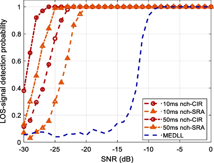

  

  Comparison of signal detection probabilities of different non-coherent accumulation durations and methods

  However, it should be noted that these two methods are not optimal estimation methods. Thus, they cannot achieve the CRLB even in high SNR scenarios.

• 2. With the increase in SNR, the RMSE of each method approaches the CRLB, multipath error and mobility error. Among the two methods, the nch-CIR has a better weak signal estimation ability. As shown in Fig. 13, with the increase in SNR, the PD of nch-CIR can reach nearly 100% 3 dB earlier than that of nch-SRA in both 10 ms and 50 ms non-coherent accumulation scenarios. In contrast, as a subspace algorithm, the nch-SRA does not suffer from CIR function distortion. Therefore, the nch-SRA has better multipath estimation ability than nch-CIR.

• 3. The mobility does not affect the availability of the non-coherent accumulation methods, and the influence on TOA estimation mainly comes from the delay variation between OFDM symbols. As seen from Figs. 9, 10 and 11, with the increase in SNR, the RMSE of nch-SRA will approach the mobility error defined by (42), while the RMSE of nch-CIR will approach the larger one of multipath error and mobility error.

• 4. Increasing the non-coherent accumulation time will not only improve the weak signal estimation ability but also increase the mobility error. After providing the analysis of computational complexity, the selection of accumulation times will be discussed in detail.

3.1.2 The results in the complex multipath channel

Through the simulation results of the previous subsection, it can clearly see the respective characteristics of the two methods. However, the real channel is much more complex than the two-path channel, and the simulations in the previous subsection cannot reflect the influence of the estimated path number ${\hat{L}}$ on the TOA estimation of the nch-SRA. Therefore, two complex multipath environments are established according to the real received signals. The configurations of these two channels are shown in Table 3. In these simulations, the speed of the receiver is set as 10 m/s, and the non-coherent accumulation time is set as 50 ms.

Table 3 Multipath configuration of the simulations

The simulation results are shown in Fig. 14. The performance comparison of the nch-CIR, the nch-SRA without covariance matrix dimension reduction (DR) and the nch-SRA with DR in complex multipath environments is given. It can be seen that without DR, the performance of the nch-SRA will degrade significantly. After matrix dimension reduction, the weak signal estimation ability of nch-SRA is improved by approximately 6 dB.

Fig. 14

Comparison of the TOA estimation performance of nch-CIR and nch-SRA with and without eigenvalue correction

In addition, in complex multipath environments, the advantage of nch-CIR’s anti-noise ability will be highlighted, but its multipath error will also be increased.

3.2 Parameter optimization

Considering the requirements of low power consumption and miniaturization for practical applications, it is necessary to reduce the computational complexity. Therefore, in this section, the computational complexity of the two methods is analyzed, and the parameter selection strategy for the two methods is explained.

It is necessary to point out that the computational complexity in this paper is defined as the total computational complexity of a TOA estimation divided by the CFR number $N_{\text{nch}}$. In addition, the reduction of computational complexity is carried out on the premise of ensuring TOA estimation accuracy.

The computational complexity of the nch-CIR algorithm is analyzed as follows. First, calculating each CIR requires $O({k_{zp}}M\log ({k_{zp}}M))$ multiplications. Then, assuming that the number of paths to be estimated is ${\hat{L}}$, $O((2{\hat{L}} + 1){N_{\text{nch}}}{k_{zp}}M)$ multiplications are needed for a TOA estimation. In summary, the equivalent computational complexity of nch-CIR is

$$\begin{aligned} O\left( {{k_{zp}}M(2{\hat{L}} + \log ({k_{zp}}M))} \right) . \end{aligned}$$

(43)

Next, the computational complexity of the nch-SRA algorithm is analyzed as follows. First, $O\left( {K{P^2}} \right)$ multiplications are needed to estimate each covariance matrix. Then, completing one SRA when $P \gg {\hat{L}}$ takes approximately $O\left( {{P^2}(K + 2{\hat{L}})} \right)$ multiplications. Since $K \gg (K + 2{\hat{L}})/{N_{\text{nch}}}$, in summary, the computational complexity of the nch-SRA algorithm is

$$\begin{aligned} O\left( {(M - P + 1){P^2}} \right) . \end{aligned}$$

(44)

A comparison of the computational complexity of the two methods and MEDLL under the assumption that ${N_c} = 2048$ is shown in Fig. 15. The complexity analysis of MEDLL can be found in [24]. The computational complexity of nch-CIR is much lower than that of nch-SRA.

Fig. 15

Computational complexity comparison between the nch-CIR and the nch-SRA

Based on (43) and (44), the discussion of the parameter selection strategy is presented as follows.

For nch-CIR, ${k_{zp}}$ is an adjustable parameter related to computational complexity, and it also determines the resolution of the CIR ${\Delta _\tau }$. When ${\Delta _\tau }$ is sufficient to meet the TOA estimation requirements, as

$$\begin{aligned} {\Delta _\tau } \leqslant {\sigma _{TOA,LB}}, \end{aligned}$$

(45)

where ${\sigma _{\text{TOA},\text{LB}}}$ is the lowest possible standard deviation of TOA estimation of the current received signal, a further increase in ${k_\text{zp}}$ will lead to a waste of computing resources. However, during the parameter setting process, the system does not know the channel characteristics. Therefore, it is assumed that no multipath is present in the received signal. This hypothesis will only lead to a larger value of ${k_\text{zp}}$ and will not reduce the TOA estimation accuracy. Then, ${\sigma _{\text{TOA},\text{LB}}}$ can be replaced as ${{\hat{\sigma }} _{{\tau _0},L = 1,\text{CRLB}}}$, and the criterion for ${k_{zp}}$ selection is as follows

$$\begin{aligned} {\Delta _\tau } \leqslant {{\hat{\sigma }} _{{\tau _0},L = 1,\text{CRLB}}}. \end{aligned}$$

(46)

Then, ${k_\text{zp}}$ is minimized as

$$\begin{aligned} {k_\text{zp}} = \text{Int}\left\{ {\frac{{{N_c}{T_s}}}{{M\Delta \text{CRS}{{{\hat{\sigma }} }^{}}_{{\tau _0},L = 1,\text{CRLB}}}}} \right\} \approx \text{Int}\left\{ {\sqrt{\frac{{2{\pi ^2}({M^2} - 1){N_{\text{nch}}}S{\hat{N}}{R_{i = 0}}}}{{3M}}} } \right\} \end{aligned}$$

(47)

where $S{\hat{N}}{R_{i = 0}}$ can be obtained according to [42], as

$$\begin{aligned} S{\hat{N}}{R_{i = 0}} = \frac{{\frac{1}{M}\sum \limits _{k = 0}^{M - 1} {{{\left| {{{{\hat{H}}}_i}[k]} \right| }^2}} - {{{\hat{\sigma }} }^2}}}{{{{{\hat{\sigma }} }^2}}}. \end{aligned}$$

(48)

and ${{\hat{\sigma }} ^2}$ can be estimated as

$$\begin{aligned} {{\hat{\sigma }} ^2} = \frac{N}{{\left( {N - 2N{'_{cp}}} \right) }}\sum \limits _{n = N{'_{cp}}}^{N - N{'_{cp}}} {{{\left| {{{{\hat{h}}}_{i = 0}}[n]} \right| }^2}} ,{\text { }}N{'_{cp}} = \text{Int}\{ \frac{{3N}}{{{N_c}}}{N_{cp}}\}. \end{aligned}$$

(49)

where ${{\hat{h}}_{i = 0,{k_\text{zp}} = 1}}[n]$ is the CIR in (11) when $i=0$, $k_\text{zp}=1$. $N_\text{cp}$, $N_{r}$ and $N_{c}$ have been introduced in Sect. 2.1.

For nch-SRA, P is the only tunable parameter. However, in practice, we found that the ESPRIT algorithm is very sensitive to the selection of P, and improper selection will significantly increase the TOA estimation error. Therefore, the adjustment of P should give priority to the TOA estimation accuracy.

In addition, based on simulations and computational complexity analysis, the selection of accumulation times should consider hardware performance, carrier dynamics and accuracy requirements. For low dynamic carriers, such as pedestrians and vehicles in cities, the number of accumulation times can be promoted as much as possible within the hardware performance. For highly dynamic carriers, such as vehicles on highways and high-speed trains, the mobility error should not exceed the maximum error that can be tolerated.

3.3 Experimental results

To evaluate the TOA estimation performance of the proposed methods, real signal ranging experiments were conducted. Aimed at TOA estimation in weak LOS environments discussed in this paper, three segments of the received signal reflecting three typical signal transmission environments are extracted. The base station locations and the movement trajectories obtained by GPS corresponding to three received signal segments are summarized in Fig. 16. The actual configurations of the LTE system in the experimental environments are shown in Table 4.

Fig. 16

Experimental environments

Table 4 LTE configuration in experimental environments

In addition, two methods are selected for comparison: the threshold method based on CA-CFAR used in [4] and the MEDLL we used in Sect. 3.1. To ensure fairness, (1) all the results are unfiltered. (2) The threshold-based method takes the non-coherent accumulated CIR as the input. (3) The MEDLL takes the average value of the TOA estimation results within the non-coherent accumulation time as the output.

Figure 17 shows the ranging results obtained from the signal segments shown in Fig. 16 based on the two methods proposed in this paper and the two comparison methods. The offset in Fig. 17 is defined as the offset of the distance between the receiver and the base station since time 0, and the GPS offset is obtained by calculating the distance between the localization result given by GPS and the base station. In Fig. 17, the cumulative distribution functions (CDFs) of the TOA estimation error are given for quantitative analyses of the experiments. Furthermore, the 50% circular error probability (CEP), 95% radius (R95) and PD of each method in each signal segment are summarized in Table 5.

Fig. 17

The comparison between the ranging results of different methods and the GPS results

After CIRs are non-coherently accumulated, the sidelobe of their function will be highlighted. When TOA estimation is carried out by the traditional threshold method in this scenario, using a high threshold will lead to a missed LOS signal, and using a low threshold may misjudge the sidelobe as the LOS signal. As shown in Fig. 17, the threshold method based on CA-CFAR cannot provide continuous and accurate TOA estimation in any signal segment. In contrast, the nch-CIR can achieve reliable TOA estimation in all signal segments due to the avoidance of sidelobe influence.

In the first signal segment, with an increasing influence of the multipath propagation and the signal power attenuation caused by the directionality of the base station antenna in the second half of the trajectory, the signal transmission channel gradually meets the weak LOS characteristics. As shown in Fig. 17a, the performance of the Avg. MEDLL decreases significantly, while the performance of the nch-CIR method also decreases slightly with the increased multipath influence. It can be seen from Table 5 that the performance degradation of the Avg. MEDLL at the end of the trajectory leads to its R95 being significantly higher than the two methods proposed in this paper.

In the second segment, occlusion sometimes occurs between the base station and the receiver. This results in the LOS signal being heavily attenuated and drowned in noise. Figure 17b shows that the performance of Avg. MEDLL is poor in this environment, and the fading LOS signal component is seldom extracted. Therefore, the error CDF of the Avg. MEDLL shown in Fig. 18b increases rapidly at approximately 50 m. In contrast, the two methods proposed in this paper can extract the LOS channel components correctly, and the ranging results are close to the GPS results. In addition, the large delay between the paths makes the nch-CIR method estimate the TOA accurately. The error CDFs of the two proposed methods are similar.

Fig. 18

The CDF calculated according to the experimental results

The signal in the third segment is subject to serious multipath interference and power attenuation. As seen from Figs. 17c and 18c, the performance of the Avg. MEDLL and nch-CIR methods in this signal segment is similar, and both of them have high estimation errors. Among them, the error of Avg. MEDLL is mainly due to the signal power attenuation which leads to the missed detection of the LOS signal, while the error of nch-CIR is mainly due to the complex multipath transmission. In comparison, the performance of nch-SRA is significantly better than the above two methods.

Table 5 Statistics of experimental results

In conclusion, the two non-coherent accumulation-based methods proposed in this paper can achieve high-precision TOA estimation and satisfactory environmental adaptability. Among them, the estimation accuracy of nch-SRA is better in complex multipath propagation environments because nch-CIR is limited by CIR function distortion.

4 Conclusion

To solve the problem that the ground localization system based on cellular signals is vulnerable to the hazards of signal power attenuation and multipath propagation in urban environments, we discuss the utilization of non-coherent accumulation for cellular TOA estimation using LTE CRS as an example. Two TOA estimation algorithms based on non-coherent accumulation were proposed. The first is the “TOA estimation algorithm based on non-coherent accumulation of the channel impulse response” (nch-CIR), and the second is the “Super Resolution TOA Estimation Algorithm based on non-coherent accumulation of the covariance matrix” (nch-SRA). Through theoretical analysis and a large number of Monte Carlo simulations, we discuss the influence of mobility on these two methods. In addition, ground localization experiments are carried out using real collected LTE signals. The results show that the two non-coherent accumulation-based methods proposed in this paper can achieve high-precision TOA estimation and satisfactory environmental adaptability. (Compared with MEDLL, the CEP of nch-SRA is reduced by 10.7%$-$44.6%, and the PD of nch-SRA is increased by 9.1%$-$17.5%.) Among these two methods, the nch-CIR algorithm has a lower computational cost and better anti-noise performance, and the nch-SRA algorithm has better performance in terms of multipath mitigation. This work will enhance the opportunistic localization approach for cellular downlink signals in urban environments.

References

M.Z. Win, A. Conti, S. Mazuelas, Y. Shen, W.M. Gifford, D. Dardari, M. Chiani, Network localization and navigation via cooperation. IEEE Commun. Mag. 49(5), 56–62 (2011). https://doi.org/10.1109/MCOM.2011.5762798
Z.Z.M. Kassas, J. Khalife, K. Shamaei, J. Morales, I hear, therefore i know where i am: compensating for GNSS limitations with cellular signals. IEEE Signal Process. Mag. 34(5), 111–124 (2017). https://doi.org/10.1109/MSP.2017.2715363
P.S. Farahsari, A. Farahzadi, J. Rezazadeh, A. Bagheri, A survey on indoor positioning systems for iot-based applications. IEEE Internet Things J. 9(10), 7680–7699 (2022). https://doi.org/10.1109/JIOT.2022.3149048
K. Shamaei, J. Khalife, Z.M. Kassas, Exploiting lte signals for navigation: theory to implementation. IEEE Trans. Wirel. Commun. 17(4), 2173–2189 (2018). https://doi.org/10.1109/TWC.2018.2789882
K. Shamaei, Z.M. Kassas, Receiver design and time of arrival estimation for opportunistic localization with 5g signals. IEEE Trans. Wirel. Commun. 20(7), 4716–4731 (2021). https://doi.org/10.1109/TWC.2021.3061985
J.A. del Peral-Rosado, R. Raulefs, J.A. López-Salcedo, G. Seco-Granados, Survey of cellular mobile radio localization methods: From 1g to 5g. IEEE Commun. Surv. Tutor. 20(2), 1124–1148 (2018). https://doi.org/10.1109/COMST.2017.2785181
K. Shamaei, Z.M. Kassas, A joint TOA and DOA acquisition and tracking approach for positioning with LTE signals. IEEE Trans. Signal Process. 69, 2689–2705 (2021). https://doi.org/10.1109/TSP.2021.3068920
S. Coleri Ergen, H.S. Tetikol, M. Kontik, R. Sevlian, R. Rajagopal, P. Varaiya, Rssi-fingerprinting-based mobile phone localization with route constraints. IEEE Trans. Vehic. Technol. 63(1), 423–428 (2014). https://doi.org/10.1109/TVT.2013.2274646
J.A. del Peral-Rosado, J.A. López-Salcedo, G. Seco-Granados, F. Zanier, M. Crisci, Evaluation of the LTE positioning capabilities under typical multipath channels, in 2012 6th Advanced Satellite Multimedia Systems Conference (ASMS) and 12th Signal Processing for Space Communications Workshop (SPSC), (2012), pp. 139–146. IEEE
F. Knutti, M. Sabathy, M. Driusso, H. Mathis, C. Marshall, et al., Positioning using LTE signals, in Proceedings of Navigation Conference in Europe, (2015), pp. 1–8
C. Yang, A. Soloviev, Positioning with mixed signals of opportunity subject to multipath and clock errors in urban mobile fading environments, in Proceedings of the 31st International Technical Meeting of the Satellite Division of The Institute of Navigation (ION GNSS+ 2018), (2018), pp. 223–243
P. Gadka, J. Sadowski, J. Stefanski, Detection of the first component of the received lte signal in the otdoa method. Wirel. Commun. Mob. Comput. 2019 (2019)
I. Sobron, I. Landa, I. Eizmendi, M. Velez, Enhanced toa estimation through tap candidate extraction for positioning in multipath channels, in 2019 IEEE 30th Annual International Symposium on Personal, Indoor and Mobile Radio Communications (PIMRC), (2019), pp. 1–6. IEEE
J.A. Del Peral-Rosado, J.A. Lopez-Salcedo, F. Zanier, G. Seco-Granados, Position accuracy of joint time-delay and channel estimators in LTE networks. IEEE Access 6, 25185–25199 (2018)
J.A. Fessler, A.O. Hero, Space-alternating generalized expectation-maximization algorithm. IEEE Trans. Signal Process. 42(10), 2664–2677 (1994)
B.H. Fleury, M. Tschudin, R. Heddergott, D. Dahlhaus, K.I. Pedersen, Channel parameter estimation in mobile radio environments using the sage algorithm. IEEE J. Select. Areas Commun. 17(3), 434–450 (1999)
M. Noschese, F. Babich, M. Comisso, C. Marshall, Multi-band time of arrival estimation for long term evolution (LTE) signals. IEEE Trans. Mob. Comput. 20(12), 3383–3394 (2020)
X. Li, K. Pahlavan, Super-resolution toa estimation with diversity for indoor geolocation. IEEE Trans. Wirel. Commun. 3(1), 224–234 (2004)
R. Schmidt, Multiple emitter location and signal parameter estimation. IEEE Trans. Antenn. Propag. 34(3), 276–280 (1986)
R. Roy, T. Kailath, Esprit-estimation of signal parameters via rotational invariance techniques. IEEE Trans. Acous. Speech Signal Process. 37(7), 984–995 (1989)
M. Driusso, F. Babich, F. Knutti, M. Sabathy, C. Marshall, Estimation and tracking of LTE signals time of arrival in a mobile multipath environment, in 2015 9th International Symposium on Image and Signal Processing and Analysis (ISPA), (2015), pp. 276–281. IEEE
M. Driusso, C. Marshall, M. Sabathy, F. Knutti, H. Mathis, F. Babich, Vehicular position tracking using LTE signals. IEEE Trans. Vehic. Technol. 66(4), 3376–3391 (2016)
K. Shamaei, Z.M. Kassas, LTE receiver design and multipath analysis for navigation in urban environments. Navigation 65(4), 655–675 (2018)
P. Wang, Y.J. Morton, Multipath estimating delay lock loop for LTE signal toa estimation in indoor and urban environments. IEEE Trans. Wirel. Commun. 19(8), 5518–5530 (2020)
P. Wang, Y.J. Morton, Improved time-of-arrival estimation algorithm for cellular signals in multipath fading channels, in 2020 IEEE/ION Position, Location and Navigation Symposium (PLANS), (2020), pp. 1358–1364. IEEE
K. Shamaei, J. Khalife, Z.M. Kassas, A joint TOA and DOA approach for positioning with LTE signals, in 2018 IEEE/ION Position, Location and Navigation Symposium (PLANS), (2018), pp. 81–91. IEEE
K. Shamaei, Z.M. Kassas, A joint TOA and DOA acquisition and tracking approach for positioning with LTE signals. IEEE Trans. Signal Process. 69, 2689–2705 (2021)
J. Qiu, Y. Qian, R. Zheng, Non-coherent, differentially coherent and quasi-coherent integration on gnss pilot signal acquisition or assisted acquisition, in Proceedings of the 2012 IEEE/ION Position, Location and Navigation Symposium, (2012), pp. 989–997. IEEE
M. Huang, W. Xu, Enhanced LTE TOA/OTDOA estimation with first arriving path detection, in 2013 IEEE Wireless Communications and Networking Conference (WCNC), (2013), pp. 3992–3997. IEEE
W. Xu, M. Huang, C. Zhu, A. Dammann, Maximum likelihood TOA and OTDOA estimation with first arriving path detection for 3g PP LTE system. Trans. Emerg. Telecommun. Technol. 27(3), 339–356 (2016)
A. Giorgetti, M. Chiani, Time-of-arrival estimation based on information theoretic criteria. IEEE Trans. Signal Process. 61(8), 1869–1879 (2013)
D. Dardari, C.-C. Chong, M. Win, Threshold-based time-of-arrival estimators in UWB dense multipath channels. IEEE Trans. Commun. 56(8), 1366–1378 (2008)
S.M. Kay, Fundamentals of Statistical Signal Processing: Estimation Theory (Prentice-Hall Inc, 1993)
Y. Tian, Y. He, H. Duan, Passive localization through channel estimation of on-the-air LTE signals. IEEE Access 7, 160029–160042 (2019)
B. Yang, K.B. Letaief, R.S. Cheng, Z. Cao, Channel estimation for OFDM transmission in multipath fading channels based on parametric channel modeling. IEEE Trans. Commun. 49(3), 467–479 (2001)
M. Wax, T. Kailath, Detection of signals by information theoretic criteria. IEEE Trans. Acoust. Speech Signal Process. 33(2), 387–392 (1985)
A.P. Liavas, P.A. Regalia, On the behavior of information theoretic criteria for model order selection. IEEE Trans. Signal Process. 49(8), 1689–1695 (2001)
Q.-T. Zhang, K.M. Wong, P.C. Yip, J.P. Reilly, Statistical analysis of the performance of information theoretic criteria in the detection of the number of signals in array processing. IEEE Trans. Acoust. Speech Signal Process. 37(10), 1557–1567 (1989)
A.P. Liavas, P.A. Regalia, J.-P. Delmas, Blind channel approximation: effective channel order determination. IEEE Trans. Signal Process. 47(12), 3336–3344 (1999)
J. Via, I. Santamaria, J. Perez, Effective channel order estimation based on combined identification/equalization. IEEE Trans. Signal Process. 54(9), 3518–3526 (2006)
H. Tian, L. Yang, S. Li, SNR estimation based on sounding reference signal in LTE uplink, in 2013 IEEE International Conference on Signal Processing, Communication and Computing (ICSPCC 2013), (2013), pp. 1–5. IEEE
Acknowledgements
Thanks to Weiming Zhong, Jialiang Sun, Zichen Song and Dr. Heliang Yuan for the assistance of the experiment and the suggestion of the article.
Funding
This work is supported by the National Natural Science Foundations of China (No. 62071020 and 61971023).
Author information
Authors and Affiliations
Contributions
All authors have contributed to the conception, design of the work, the acquisition, analysis and interpretation of data and have edited and approved the submitted version. All authors read and approved the final manuscript.
Corresponding author
Ethics declarations
Competing interests
The authors declare that they have no competing interests.
Additional information
Publisher's Note
Springer Nature remains neutral with regard to jurisdictional claims in published maps and institutional affiliations.
Rights and permissions
Open Access This article is licensed under a Creative Commons Attribution 4.0 International License, which permits use, sharing, adaptation, distribution and reproduction in any medium or format, as long as you give appropriate credit to the original author(s) and the source, provide a link to the Creative Commons licence, and indicate if changes were made. The images or other third party material in this article are included in the article's Creative Commons licence, unless indicated otherwise in a credit line to the material. If material is not included in the article's Creative Commons licence and your intended use is not permitted by statutory regulation or exceeds the permitted use, you will need to obtain permission directly from the copyright holder. To view a copy of this licence, visit http://creativecommons.org/licenses/by/4.0/.
About this article
Cite this article
Tian, J., Fangchi, L., Yafei, T. et al. Utilization of non-coherent accumulation for LTE TOA estimation in weak LOS signal environments. J Wireless Com Network 2023, 38 (2023). https://doi.org/10.1186/s13638-023-02248-1
Received:
Accepted:
Published:
DOI: https://doi.org/10.1186/s13638-023-02248-1