A distributed power control and mode selection algorithm for D2D communications

Abstract

Device-to-device (D2D) communications underlaying a cellular infrastructure has recently been proposed as a means of increasing the resource utilization, improving the user throughput and extending the battery lifetime of user equipments. In this article we propose a new distributed power control algorithm that iteratively determines the signal-to-noise-and-interference-ratio (SINR) targets in a mixed cellular and D2D environment and allocates transmit powers such that the overall power consumption is minimized subject to a sum-rate constraint. The performance of the distributed power control algorithm is benchmarked with respect to the optimal SINR target setting that we obtain using the Augmented Lagrangian Penalty Function method. The proposed scheme shows consistently near optimum performance both in a single-input-multiple-output and a multiple-input-multiple-output setting. We also propose a joint power control and mode selection algorithm that requires single cell information only and clearly outperforms the classical cellular mode operation.

Introduction

Device-to-device (D2D) communications in cellular spectrum supported by a cellular infrastructure holds the promise of three types of gains. The reuse gain implies that radio resources may be simultaneously used by cellular as well as D2D links thereby tightening the reuse factor even of a reuse-1 system [1–3]. Secondly, the proximity of user equipments (UE) may allow for extreme high bit rates, low delays and low power consumption [4]. Finally, the hop gain refers to using a single link in the D2D mode rather than using an uplink and a downlink resource when communicating via the access point in the cellular mode. Additionally, D2D communications may increase the reliability of cellular communications [5] and also facilitate new types of wireless peer-to-peer [3, 6, 7] and multicast services [8].

Although the idea of enabling D2D communications as a means of relaying in cellular networks was proposed by some early works on ad hoc networks [9, 10], the concept of allowing local D2D communications to (re)use cellular spectrum resources simultaneously with ongoing cellular traffic is relatively new [2, 3, 11, 12]. Because the non-orthogonal resource sharing between the cellular and the D2D layers has the potential of the reuse gain, proximity gain and hop gain and at the same time increasing the resource utilization [13–15], D2D communications underlaying cellular networks has received considerable interest in the recent years.

A series of articles analyzes and evaluates the single (isolated) cell scenario in a single-input-single-output (SISO) system to provide some basic insight into the impact of power control and resource (e.g. OFDM resource block) allocation [16–19]. The multi-cell problem scenario is considered in, for example [20], that assumes that the base station (BS) has all the involved channel state information (CSI) to select the optimal resource sharing mode (D2D mode reusing cellular resources, D2D mode using orthogonal resources and cellular mode in which the D2D pair communicates through the cellular BS). The heuristic mode selection (MS) algorithm proposed in [20] uses probing signals between the D2D transmitter and receiver to estimate the interference plus noise power and the BS has the task to estimate the transmit power, SINR and throughput in each possible communication modes on a small time scale matching with that of the transmission time interval. As stated by Doppler et al. [20], their proposed method has significant signaling load though it is expected to be feasible in low mobility scenarios. In other articles dealing with MS [15–17], the problem is addressed as finding the optimal mode for communication in terms of highest achieved rate, which requires the evaluation of the rate in all of the considered communication modes. Xiao et al. [18] proposed heuristics for joint subcarrier allocation, power control and MS to minimize the total downlink transmission power in a single-cell SISO system.

Gu et al. [21] studied a multi-cell system focusing on a SISO power control scheme that helps minimize the interference from the D2D layer to the cellular users and assuming that D2D users operate in D2D mode reusing cellular resources. D2D communication in MIMO systems is considered in [22], where interference-avoiding precoding schemes are proposed for downlink MIMO transmissions in the presence of intra-cell D2D links. In [23], a new interference management strategy is proposed to enhance the overall capacity of cellular networks and D2D systems when the BS equipped with multiple antennas enables multiple cellular UEs to communicate simultaneously with the help of MIMO spatial multiplexing techniques.

Since the main motivation and justification of allowing D2D communications in cellular spectrum is ultimately to harvest some capacity, sum-rate or sum-power gain, many articles apply optimization techniques to explore the potential of cellular D2D communications [14–16, 19]. These works provide important reference cases when the assumption can be made that the BS is aware of the CSI not only between transmitter-receiver pairs, but also of the interference links, such as, for example the state of the link between the D2D transmitter and the cellular receiver (BS) and/or the cellular transmitter (e.g. cellular UE) and the D2D receiver.

Typically, state of the art works give priority to the cellular users or avoids or constraints the interference caused by the D2D users to the cellular layer, see for example [15–17, 22–26]. However, it can be argued that D2D traffic should be treated near equally to the cellular traffic as long as fairness between all cellular spectrum users (i.e. cellular and D2D users) are handled [27, 28], since they all use cellular spectrum under operator controlled charging conditions.

In this article, our purpose is to propose and study the joint performance of a practically viable power control and MS algorithm applicable in multicell cellular systems supporting D2D communications, such that the algorithms use only limited CSI. To this end, we only require that the receiver nodes can estimate (measure) the covariance of the total received interference and feed it back to their respective transmitters. This piece of information is then used by the transmitters in a distributed fashion to adjust their respective transmit powers such that some predefined SINR targets are reached. Next, this basic algorithm can be optionally combined with an SINR target setting algorithm that allows to minimize the overall used power subject to some sum rate target such that a minimum link quality is also guaranteed for both the cellular and the D2D transmission links. Finally, we also propose a practical MS algorithm that only requires the CSI (specifically the large scale fading) information of the useful and interfering links in the own cell.

To gain insight into the behavior of the iterative distributed power control scheme, we study a small system in which we calculate the local optimum power setting assuming full channel knowledge and compare the performance of the heuristic iterative method relying on the D2D geometry (i.e. large scale fading information) with that of the scheme that provides the local optimum. We are also interested in gaining insight in the potential gains of using the direct D2D link as compared to using cellular links between two communicating UEs (Tx UE–Rx UE) when employing such power control in both (i.e. cellular and D2D) operational modes. In particular, we focus on scenarios in which the same PRB may be used simultaneously for a cellular and a D2D link tightening the reuse factor below 1 (as in Figure 1). For a particular UE pair, this sum power minimizing scheme may be combined with MS that determines whether a particular UE pair—the D2D candidate: Tx UE–Rx UE of Figure 1—should use the direct D2D link or they should communicate via the cellular access point [29]. Therefore, we compare the performance of these two communications modes when the positions of both the D2D pair and the interfering cellular UE vary within the cell.

Figure 1

Illustration of D2D communications, when a user equipment (UE1) and a D2D pair (Tx UE–Rx UE) may use the same OFDM PRB. Due to the D2D link, intracell interference as well as intercell interference between D2D and cellular links (UE3 to Rx UE) can be very high. (In this example assuming that the D2D link uses cellular UL resources).

The current article is a substantially revised and extended version of [30]^a. First, we revised the distributed power control algorithm (Algorithm 1) such that it is based on the measured covariance of the total received interference and noise and investigate the impact of the measurement error. Second, the description of the optimum power allocation method using the augmented Lagrangian penalty function (ALPF) scheme has been revised and illustrated through a specific numerical example. Also, in this article, we provide the detailed derivations of the steps needed in the SINR target setting scheme (Algorithm 2). Third, we introduce a practical MS algorithm that requires only average CSI information from the own cell. Furthermore, new numerical results are presented to evaluate the potential gains of D2D communications under strong and weak intercell interference situations. Finally, the performance of the distributed power control scheme with and without adaptive SINR target adjustment is evaluated jointly with the proposed MS algorithm in various parameter configurations of a 7-cell system.

Our scheme does not consider the scheduling or pairing problem that is concerned with selecting the specific cellular users and D2D pairs and allocating OFDM resource blocks or subcarriers to them [13, 15, 27, 31–33]. Therefore, we believe that our work can be an efficient complement to these resource allocation and pairing schemes.

We structure the article as follows. The next section describes our system model and formulates the D2D power control problem as an optimization task. Next, in Section “An iterative D2D power control scheme”, we propose an iterative power control scheme to meet predefined SINR targets. A second algorithm is presented in Section “Determining the optimum SINR target” that aims to set the SINR targets that help to minimize the overall used power in the system. In Section “Mode selection”, the proposed MS algorithm is presented that relies on single cell information and dynamically selects between cellular and D2D communication modes. Section “Numerical results” discusses numerical results and Section “Conclusions” highlights our findings.

Throughout the article, we use the following notations. A⁻¹, A^T and A^Hdenote the pseudo-inverse, the transpose and the conjugate transpose of matrix A, respectively. {A}^(i,j) is the (i,j)^th element of matrix A, while diag(a₁,…,a _N ) denotes a N × N diagonal matrix whose diagonal elements are the scalars a₁,…,a _N . The absolute value of a real or complex number z is denoted by |z|. Furthermore, trace(·) and $\mathbb{E}(·)$ represent the trace and the expectation operations of matrix A, respectively.

System model

Modeling the received signal

We focus on the case in which a cellular and a D2D link are multiplexed on the same uplink OFDM PRB.^b Due to intercell interference, cellular or D2D links in neighboring cells may cause additional interference to the received signal. Thus, the received signal at the k th receiver (i.e. cellular AP or the Rx UE of a D2D pair) can be modeled as:

$${\mathbf{y}}_k={\alpha }_{k,k}{\mathbf{H}}_{k,k}{\mathbf{T}}_k{\mathbf{x}}_k+\sum _{j\ne k}{\alpha }_{k,j}{\mathbf{H}}_{k,j}{\mathbf{T}}_j{\mathbf{x}}_j+{\mathbf{n}}_k,$$

(1)

where

• N _t is the number of transmit antennas and N _r is the number of receive antennas;

• ${\alpha }_{k,j}=\sqrt{P_j{d}_{k,j}^{-{\rho }_{k,j}}{\chi }_{k,j}/N_t}$ is a scalar coefficient depending on the total transmit power P _j for user j, the log-normal shadow fading χ_k,jand distance d_k,jbetween the k th receiver and the j th transmitter with path loss exponent ρ_k,j. The values of ρ_k,jand χ_k,jdepend on the transmitter and receiver being a transmitter UE, a receiver UE or a cellular access point respectively, the specific environment (e.g. indoor or outdoor deployment, femto or macro type of access point), etc.

• ${\mathbf{x}}_k\in {\mathbb{C}}^{N_t\times 1}$ is the data vector that is assumed to be zero-mean, normalized and uncorrelated, $\mathbb{E}\left({\mathbf{x}}_k{\mathbf{x}}_k^{†}\right)={\mathbf{I}}_{N_t}$;

• H_k,jdenotes the (N _r  × N _t )channel transfer matrix; and

• T _k is the UE-k(N _t  × N _t )diagonal power loading matrix. To keep the total transmit power constant, T _k must satisfy

  $$\text{trace}\left({\mathbf{T}}_k{\mathbf{T}}_k^{†}\right)=\sum _{i=1}^{N_t}|{\left\{{\mathbf{T}}_k\right\}}^{(i,i)}{|}^2=N_t\forall k;$$

n _k is a N _r  × 1 additive white Gaussian noise vector at the k th receiver with zero mean and covariance matrix ${\mathbf{R}}_{n_k}=\mathbb{E}\left({\mathbf{n}}_k{\mathbf{n}}_k^{†}\right)={\sigma }_n^2{\mathbf{I}}_{N_r}\forall k$.

We rewrite the signal model (1) in a compact form as

$${\mathbf{y}}_k={\alpha }_{k,k}{\mathbf{H}}_{k,k}{\mathbf{T}}_k{\mathbf{x}}_k+{\mathbf{z}}_k+{\mathbf{n}}_k,$$

(2)

where ${\mathbf{z}}_k=\sum _{j\ne k}{\alpha }_{k,j}{\mathbf{H}}_{k,j}{\mathbf{T}}_j{\mathbf{x}}_j$ denotes the (N _r  × 1) interference vector with covariance matrix

$${\mathbf{R}}_{z_k}=\mathbb{E}\left({\mathbf{z}}_k{\mathbf{z}}_k^{†}\right)=\sum _{j\ne k}{\alpha }_{k,j}^2{\mathbf{H}}_{k,j}{\mathbf{T}}_j{\mathbf{T}}_j^{†}{\mathbf{H}}_{k,j}^{†}.$$

(3)

For ease of notation, we define an equivalent noise vector that accounts for both the inter-cell interference and the background noise:

$${\mathbf{v}}_k={\mathbf{z}}_k+{\mathbf{n}}_k$$

It is easy to show that v _k is zero-mean with covariance ${\mathbf{R}}_{v_k}={\mathbf{R}}_{z_k}+{\mathbf{R}}_{n_k}$.

MMSE receiver error matrix and the effective SINR

In what follows we revise and merge the methods followed by [34–36] to calculate the MMSE receiver error matrix and the effective SINR. We assume that the received signal both at the AP and the Rx UE is filtered through a linear MMSE receiver with weighting matrix G _k to obtain the estimate

$${\hat{\mathbf{x}}}_k={\mathbf{G}}_k{\mathbf{y}}_k.$$

where the (N _t  × N _r ) linear MMSE weighting matrix G _k is given as:

$$\begin{array}{l}{\mathbf{G}}_k=\frac{1}{{\alpha }_{k,k}}{\mathbf{T}}_k^{†}{\mathbf{H}}_{k,k}^{†}{\left({\mathbf{H}}_{k,k}{\mathbf{T}}_k{\mathbf{T}}_k^{†}{\mathbf{H}}_{k,k}^{†}+\frac{1}{{\alpha }_{k,k}^2}{\mathbf{R}}_{v_k}\right)}^{-1}\\ ={\left(\mathbf{I}+{\mathbf{T}}_k^{†}{\mathbf{R}}_{H_k}{\mathbf{T}}_k\right)}^{-1}{\alpha }_{k,k}{\mathbf{T}}_k^{†}{\mathbf{H}}_{k,k}^{†}{\mathbf{R}}_{v_k}^{-1},\end{array}$$

where ${\mathbf{R}}_{H_k}={\alpha }_{k,k}^2{\mathbf{H}}_{k,k}^{†}{\mathbf{R}}_{v_k}^{-1}{\mathbf{H}}_{k,k}$, see e.g. ([37], Chapter 12).

To derive the stream-wise SINRs at BS k, we will need the diagonal elements of the error matrix of the MMSE filtered signal. To this end, the following known result (see e.g. [34–36] and ([37], Chapter 12)) is useful. (The derivation is provided in Appendix 1: derivation of the MMSE estimation error matrix). The MMSE estimation error matrix (N _r  × N _r )for the k th BS is:

$$\begin{array}{ll}{\mathbf{E}}_k& ={\left(\mathbf{I}+{\mathbf{T}}_k^{†}{\mathbf{R}}_{H_k}{\mathbf{T}}_k\right)}^{-1}.\end{array}$$

(4)

We are now in the position to calculate the SINR for the signal model (2) assuming a linear MMSE receiver. Using the linear MMSE weighting matrix G _k , the MSE and SINR expressions can be rewritten, respectively as

$$\begin{array}{l}{\text{MSE}}_{k,s}\triangleq {\left\{{\mathbf{E}}_k\right\}}^{(s,s)}={\left\{{\left(I+{\mathbf{T}}_k^{†}{\mathbf{R}}_{H_k}{\mathbf{T}}_k^{†}\right)}^{-1}\right\}}^{(s,s)},\end{array}$$

(5)

$$\begin{array}{l}{\gamma }_{k,s}\triangleq \frac{1}{{\mathrm{MSE}}_{k,s}}-1.\end{array}$$

(6)

Summary

In this section we defined the multicell MIMO received signal model (2) and, assuming a linear MMSE receiver, derived the associated effective SINR (γ_k,s) for each stream of the received signal. Equations (5) and (6) are important because they capture the dependence of the SINRs on the transmission powers of the own UE and the interfering UEs (both at an access point and at a receiving UE of a D2D pair) through the ${\mathbf{R}}_{H_k}$’s and the ${\mathbf{R}}_{v_k}$’s. Thus, these relations serve as the basis for the optimization problems of the next section.

An iterative D2D power control scheme

From the signal model (1), when transmitter k uses a diagonal power loading matrix ${\mathbf{T}}_k\in C^{N_t\times N_t}$ with $\sum _{s=1}^{N_t}\mid {\left\{{\mathbf{T}}_k\right\}}^{(s,s)}{\mid }^2=N_t$, the post-processing SINR of its s th stream becomes [36]:

$$\begin{array}{l}{\gamma }_{k,s}=\frac{P_k\mid {\left\{{\mathbf{T}}_k\right\}}^{(s,s)}{\mid }^2}{{\zeta }_{k,s}}-1,\end{array}$$

(7)

where

$$\begin{array}{ll}{\zeta }_{k,s}& =\left\{\left(d_{k,k}^{-\rho }{\chi }_{k,k}{\mathbf{H}}_{k,k}^{†}\left(\sum _{j\ne k}{P}_j{d}_{k,j}^{-\rho }{\chi }_{k,j}{\mathbf{H}}_{k,j}{\mathbf{T}}_j{\mathbf{T}}_j^{†}{\mathbf{H}}_{k,j}^{†}\right.\right.\right.\\ +{\left.{\left.{\left.N_t{\sigma }_n^2{\mathbf{I}}_{N_r\times N_r}\right)}^{-1}{\mathbf{H}}_{k,k}+\frac{1}{P_k}{\mathbf{I}}_{N_t\times N_t}\right)}^{-1}\right\}}^{(s,s)}\end{array}$$

(8)

denotes the effective interference after MMSE processing and {·}^(i,j) denotes the operation of acquiring the matrix element of the i th row of the j th column. In [36], a heuristic algorithm for distributing the transmit power over different streams was presented. By inverting Equation (7) for fixed SINR targets, the algorithm finds a near optimal (sum power minimizing) power loading matrix for these given SINR targets assuming perfect knowledge of the own and cross channel matrices H_k,j.

Unfortunately, in the mixed cellular and D2D communications scenario, the availability of the cross channel matrices at the transmitters cannot be assumed, because that would require extensive reference signal processing and channel quality information reporting. Therefore, in this article, we relax the assumption on the knowledge of all the H_k,j channel matrices at all transmitters. Our assumption instead is that Receiver-k estimates the covariance of the total received signal and noise (Φ _k ) and feeds it back to its transmitter. We further assume that Transmitter-k knows its channel to its receiver (H_k,k), which is reasonable considering that in practice a D2D pair typically communicates over a bidirectional channel and that the D2D link can be expected to operate in a time division duplex (TDD) mode [3, 24].

The Φ _k as measured by Receiver-k and fed back to the transmitter can then be expressed as:

$${\mathbf{\Phi }}_k=\sum _{j=1}^K{P}_j{d}_{k,j}^{-\rho }{\chi }_{k,j}{\mathbf{H}}_{k,j}{\mathbf{T}}_j{\mathbf{T}}_j^{†}{\mathbf{H}}_{k,j}^{†}+N_t{\sigma }_n^2{\mathbf{I}}_{N_{r}x{N}_r};$$

(9)

from which Transmitter-k simply needs to subtract its own contribution, i.e.

$$P_k{d}_{k,k}^{-\rho }{\chi }_{k,k}{\mathbf{H}}_{k,k}{\mathbf{T}}_k{\mathbf{T}}_k^{†}{\mathbf{H}}_{k,k}^{†}.$$

(10)

Transmitter-k can then calculate the effective interference ζ after the MMSE processing based on (8).

The covariance estimation based iterative power control algorithm is summarized by the pseudo code of Algorithm 1. (In practice, the receiver can estimate the covariance matrix of the received interference-plus-noise and feed back this reduced covariance matrix ${\mathbf{\Phi }}_k^{\mathrm{red}}$ as defined in Algorithm 1.) Algorithm 1 iteratively adjusts the power loading matrix T _k such that the MIMO streams that suffer from higher effective interference ζ are allocated higher transmit power, since the given fixed SINR target $\mathit{\Gamma }\triangleq \text{diag}\left({\gamma }_1^{\mathrm{tgt}},\dots ,{\gamma }_K^{\mathrm{tgt}}\right)$ where ${\gamma }_k^{\mathrm{tgt}}$ is the assumed given SINR target at Receiver-k is set equal to all streams of Transmitter-k. Without unequal power loading, when the “weakest” stream’s SINR is raised to the target, the stronger streams tend to overshoot the SINR target and thereby to waist transmit power. The transmit power itself (P _k ) is determined by the MIMO stream that requires the highest transmit power (proportional to the effective interference and target SINR (${\gamma }_k^{\mathrm{tgt}}$)).

Algorithm 1 Iterative transmit power and power loading optimization

Given t = 0(iteration number), P_tot, ϵ_gap and ${\mathbf{T}}_k^{\left(0\right)}={\mathbf{I}}_{N_t}\forall k$. {·}^(i,j) denotes the operation of acquiring the matrix element of the i^throw of the j^thcolumn.

Initialize SINR targets ${\mathit{\Gamma }}^{\left(0\right)}=\text{diag}\left({\gamma }_k^{\mathrm{tgt}}\right)$, where ${\gamma }_k^{\mathrm{tgt}}$ is the assumed given SINR target at Receiver-k, and initial transmit powers p⁽⁰⁾.

Repeat

• 1. t = t + 1.

• 2. for k = 1 to K do

Receiver-k measures the Φ _k as:

$$\begin{array}{ll}{\mathbf{\Phi }}_k^{\left(t\right)}& =\sum _{j=1}^K{P}_j^{(t-1)}{d}_{k,j}^{-\rho }{\chi }_{k,j}{\mathbf{H}}_{k,j}{\mathbf{T}}_j^{(t-1)}{\mathbf{T}}_j^{(t-1)†}{\mathbf{H}}_{k,j}^{†}\\ +N_t{\sigma }_n^2{\mathbf{I}}_{N_{r}x{N}_r};\end{array}$$

(11)

Receiver-k feeds the estimated (measured) Φ _k back to Transmitter-k;

Transmitter-k calculates the reduced ${\mathbf{\Phi }}_k^{\mathrm{red}}$ as:

$$\begin{array}{ll}{\mathbf{\Phi }}_k^{\mathrm{red},\left(t\right)}& ={\mathbf{\Phi }}_k^{\left(t\right)}-P_k^{(t-1)}{d}_{k,k}^{-\rho }{\chi }_{k,k}{\mathbf{H}}_{k,k}{\mathbf{T}}_k^{(t-1)}{\mathbf{T}}_k^{(t-1)†}{\mathbf{H}}_{k,k}^{†}\\ =\sum _{j\ne k}{P}_j^{(t-1)}{d}_{k,j}^{-\rho }{\chi }_{k,j}{\mathbf{H}}_{k,j}{\mathbf{T}}_j^{(t-1)}{\mathbf{T}}_j^{(t-1)†}{\mathbf{H}}_{k,j}^{†}\\ +N_t{\sigma }_n^2{\mathbf{I}}_{N_{r}x{N}_r};\end{array}$$

(12)

Transmitter-k calculates the effective interference ζ_k,sas:

$$\begin{array}{ll}{\zeta }_{k,s}^{\left(t\right)}& =\left\{\left(d_{k,k}^{-\rho }{\chi }_{k,k}{\mathbf{H}}_{k,k}^{†}{\left({\mathbf{\Phi }}_k^{\mathrm{red},\left(t\right)}\right)}^{-1}{\mathbf{H}}_{k,k}\right.\right.\\ +{\left.{\left.\frac{1}{P_k^{(t-1)}}{\mathbf{I}}_{{\mathbf{N}}_{\mathbf{t}}{\mathbf{xN}}_{\mathbf{t}}}\right)}^{-1}\right\}}^{(s,s)};\end{array}$$

(13)

Transmitter-k calculates the optimum loading matrix ${\mathbf{T}}_k^{\left(t\right)}$ and P _k as:

$$\begin{array}{l}{\left\{{\mathbf{T}}_k^{\left(t\right)}\right\}}^{(s,s)}=\sqrt{\frac{{\zeta }_{k,s}^{\left(t\right)}{N}_t}{{\sum }_{w=1}^{N_t}{\zeta }_{k,w}^{\left(t\right)}}},\forall s\in [1,N_t];\end{array}$$

$$\begin{array}{l}{P}_k^{\left(t\right)}=\underset{s}{max}\left\{\frac{{\zeta }_{k,s}^{\left(t\right)}}{{\left|{\left\{{\mathbf{T}}_k^{\left(t\right)}\right\}}^{(s,s)}\right|}^2}\left({\gamma }_k^{\mathrm{tgt}}+1\right)\right\};\end{array}$$

(14)

end

until $\mid P_k^{\left(t\right)}-P_k^{(t-1)}\mid \le {ϵ}_{\mathrm{gap}},\forall k;$

In a practical implementation, Algorithm 1 could be executed on a slower time scale relaxing the requirement on the receiver feedback. Studying the impact of the time scale for this algorithm as well as modeling delays and measurement errors are actually interesting future research topics. However, we have evaluated the performance of Algorithm 1 in one example scenario with tree transmitters and receivers (illustrated in Figure 2) when Gaussian measurement error is added to the covariance matrix estimation in (11) as ${\mathbf{\Phi }}_k^{\left(t\right)\prime }={\mathbf{\Phi }}_k^{\left(t\right)}+{\mathbf{E}}_{N_r\times N_r}^{\left(t\right)}$, where ${\left\{{\mathbf{E}}_{N_r\times N_r}^{\left(t\right)}\right\}}^{(i,j)}\sim \mathrm{N}(0,c_{\mathrm{err}}·|{\left\{{\mathbf{\Phi }}_k^{\left(t\right)}\right\}}^{(i,j)}\left|\right)$. Figure 3 shows the impact of the measurement error on the performance of Algorithm 1 in the function of the number of iterations when c_erris set to 0.2. The terms with “+ E” correspond to the cases when the measurement error is added to ${\mathbf{\Phi }}_k^{\left(t\right)}$. These curves show fluctuations around the curves with no error, but they still converge to the optimal values in this case. The convergence of Algorithm 1 is not analyzed in this article although the numerical results indicate that the algorithm converges within less than 10 iterations when the problem is feasible (see Sections “2-cell system results” and “7-cell system results”) even if measurement error is also considered (see Figure 3).

Figure 2

One Monte Carlo realization is shown with two cellular BSs and one D2D pair. Cellular UE1 is dropped in interval (5·r,6·r], where r=25 m.

Figure 3

The performance of Algorithm 1 is shown in the function of the number of iterations when Gaussian measurement error is added to the estimation of the covariance matrix. The terms with “+ E” correspond to the cases where erroneous covariance matrix is applied (c_err = 0.2).

Determining the optimum SINR target

Determining the optimum SINR target is useful for benchmarking purposes. For smaller systems, in which the number of interfering transmitters is limited, it is possible to determine the optimum SINR targets by the method we apply in this section. For larger systems, the distributed algorithm of the next section is more practical. We note that, in this section, we assume full and perfect channel knowledge at each transmitter.

Notation and assumptions for optimum SINR target setting

To formulate the SINR target setting task as an optimization problem stated in the standard form of constrained minimization [38], we make the following considerations. First, we would like to express the sum transmit power as a closed form function of the SINR targets. To this end, the following result from [36] will be useful: by assuming equal power allocation for all streams s (i.e. no uplink beam forming, ${\mathbf{T}}_k={\mathbf{I}}_{N_t}\forall k$), the minimum stream SINR at Receiver-k (a cellular access point or a D2D receiver) is lower bounded as

$$\begin{array}{l}\underset{s\in [1,N_t]}{min}{\gamma }_{k,s}\ge {\gamma }_k\left(\mathbf{p}\right)\end{array}$$

(15)

where $\mathbf{p}={\left(P_1\dots P_K\right)}^T$ is the power allocation vector, and

$$\begin{array}{l}{\gamma }_k\left(\mathbf{p}\right)=\frac{P_k{d}_{k,k}^{-\rho }{\chi }_{k,k}}{\sum _{j\ne k}{P}_j{d}_{k,j}^{-\rho }{\chi }_{k,j}{\mu }_{max}\left({\mathit{\Omega }}_{k,j,1}\right)+N_t{\sigma }_k^2{\mu }_{max}\left({\mathit{\Omega }}_{k,j,2}\right)}.\end{array}$$

(16)

Here, μ_max(·) is the maximum eigenvalue operator for a Hermitian matrix, while Ω_k,j,1and Ω_k,j,2 are defined as

$$\begin{array}{ll}{\mathit{\Omega }}_{k,j,1}& ={\left({\mathbf{H}}_{k,k}^{†}{\mathbf{H}}_{k,k}\right)}^{-1}{\mathbf{H}}_{k,k}^{†}{\mathbf{H}}_{k,j}{\mathbf{H}}_{k,j}^{†}{\mathbf{H}}_{k,k}{\left({\mathbf{H}}_{k,k}^{†}{\mathbf{H}}_{k,k}\right)}^{-1},\end{array}$$

(17)

$$\begin{array}{ll}{\mathit{\Omega }}_{k,j,2}& ={\left({\mathbf{H}}_{k,k}^{†}{\mathbf{H}}_{k,k}\right)}^{-1}.\end{array}$$

(18)

This bound allows to associate a single SINR value

$$\begin{array}{l}{\gamma }_k\left(\mathbf{p}\right)\triangleq \underset{s\in [1,N_t]}{min}{\gamma }_{k,s}\end{array}$$

(19)

with each MS-k. In what follows, we search for SINR targets ${\gamma }_k^{\text{tgt}}$ which are feasible for the lower-bound (and hence for each individual stream) and $\mathit{\Gamma }\triangleq \text{diag}({\gamma }_1^{\mathrm{tgt}}\dots {\gamma }_K^{\mathrm{tgt}})$.

Minimizing the sum power under predetermined fixed SINR targets

The above result is used in [36] to design power control schemes that maintain a predetermined fixed SINR target ${\gamma }_k^{\mathrm{tgt}}$ at each Receiver-k by enforcing ${\underset{̲}{\gamma }}_k\left(\mathbf{p}\right)\ge {\gamma }_k^{\mathrm{tgt}}$ for each user. Specifically, to reach this SINR target, the transmit power of MS-k must satisfy:

$$\begin{array}{l}{P}_k\ge {\gamma }_k^{\mathrm{tgt}}\\ ·\left(\frac{\sum _{j\ne k}{P}_j·d_{k,j}^{-\rho }{\chi }_{k,j}{\mu }_{max}\left({\mathit{\Omega }}_{k,j,1}\right)+{\sigma }_n^2{N}_t{\mu }_{max}\left({\mathit{\Omega }}_{k,j,2}\right)}{d_{k,k}^{-\rho }{\chi }_{k,k}}\right)\end{array}$$

(20)

We now make the following observation. Since the minimum user-stream SINR bound (15) allows to associate a single SINR target per user, one can regard each MS–BS or MS-D2D Rx connection as an equivalent SISO system and model the minimum user-stream capacity as function of the power allocation with a Shannon-like expression (normalized to the bandwidth) as

$$\begin{array}{l}{c}_k\left({\gamma }_k^{\mathrm{tgt}}\right)=\underset{2}{log}\left(1+{\gamma }_k^{\mathrm{tgt}}\right)\forall k,\end{array}$$

(21)

where we enforce

$$\begin{array}{l}{\underset{̲}{\gamma }}_k\left(\mathbf{p}\right)=\frac{P_k}{n_k+\sum _{j\ne k}{G}_{\mathrm{kj}}{P}_j}\ge {\gamma }_k^{\mathrm{tgt}}\forall k,\end{array}$$

(22)

with G = I + F, where n is a K dimensional effective noise variance vector whose k th element is $n_k=\frac{N_t{\sigma }_n^2{\mu }_{max}\left({\mathit{\Omega }}_{k,j,2}\right)}{d_{k,k}^{-\rho }{\chi }_{k,k}}$, and

$$\begin{array}{ll}{\mathbf{F}}_{k,j}& =\left\{\begin{array}{ll}\frac{d_{k,j}^{-\rho }{\chi }_{k,j}{\mu }_{max}\left({\mathit{\Omega }}_{k,j,1}\right)}{d_{k,k}^{-\rho }{\chi }_{k,k}}& k\ne j\\ 0& k=j;\end{array}\right.\end{array}$$

(23)

This observation is the basis for determining the SINR targets such that the sum transmit power is minimized, as shown in the next section.

The problem of optimal SINR target selection

Let c_mdenote the target sum rate of all (cellular and D2D) links over all cells in the system and c _k denote the sustainable transmission rate of link-k. With the explicit relationship between the SINR targets and the transmit powers ((16) and (20)) in hand, we can now formulate the problem of setting the SINR targets (for each receiver in the mixed cellular/D2D environment) such that the sum power is kept at a minimum level and the overall system capacity (sum rate) target c_m is reached. This problem is formulated as follows:

$$\begin{array}{l}\begin{array}{ll}\underset{\mathit{\Gamma },\mathbf{p}}{\text{minimize}}& \sum _k{P}_k\\ \text{subject to}& \sum _k{c}_k\left({\gamma }_k^{\mathrm{tgt}}\right)=c_{\mathrm{m}}\\ {\gamma }_k^{\mathrm{tgt}}={\gamma }_k\left(\mathbf{p}\right)& \forall k,\end{array}\end{array}$$

(24)

in the optimization variables $\mathit{\Gamma }\triangleq \text{diag}({\gamma }_1^{\mathrm{tgt}}\dots {\gamma }_K^{\mathrm{tgt}})$ (SINR targets) and p (transmit power).

Solution approach: employing the ALPF

We propose to solve the problems formulated in Section “The problem of optimal SINR target selection” through the ALPF method [38]. In this method, the constrained non-linear optimization task is transformed into an unconstrained problem by adding a penalty term to the Lagrangian function as follows:

$$\begin{array}{ll}\varphi (\mathit{\Gamma },\mathbf{p},\mu ,ϵ)& =L(\mathit{\Gamma },\mathbf{p},\mu )+ϵ\left[{\left(\sum _k{c}_k\left({\gamma }_k^{\mathrm{tgt}}\right)-c_{\mathrm{m}}\right)}^2\right]\\ =\sum _k{P}_k+\mu \left(\sum _k{c}_k\left({\gamma }_k^{\mathrm{tgt}}\right)-c_{\mathrm{m}}\right)\\ +ϵ\left[{\left(\sum _k{c}_k\left({\gamma }_k^{\mathrm{tgt}}\right)-c_{\mathrm{m}}\right)}^2\right],\end{array}$$

where μ is the Lagrange multiplier and ϵ is the so called penalty parameter.

It can be shown that if the optimum Lagrange multipliers are known, the solution to this unconstrained problem corresponds to the solution of the original problem (24) regardless of the value of the penalty parameter ϵ, see e.g. ([38], Chapter 9). Since we obviously do not know the value of the Lagrange multiplier, we start with an arbitrary value (e.g. zero) and develop a procedure that moves the multiplier closer to its optimum value. This procedure is detailed in the following subsection.

Updating the lagrange multipliers

Updating the Lagrange multipliers in the ALPF method hinges on comparing the necessary conditions for the minimum of the Lagrangian function and the ALPF as follows. By taking the derivative of the Lagrangian function, we obtain:

$$\frac{\mathrm{\partial L}}{\partial {\gamma }_j^{\mathrm{tgt}}}=0\Rightarrow \frac{\partial \sum _k{P}_k}{\partial {\gamma }_j^{\mathrm{tgt}}}+\mu \frac{\partial }{\partial {\gamma }_j^{\mathrm{tgt}}}\left(\sum _k{c}_k\left({\gamma }_k^{\mathrm{tgt}}\right)-c_{\mathrm{m}}\right)=0.$$

The derivative of the corresponding ALPF is:

$$\begin{array}{l}\frac{\varphi }{\partial {\gamma }_j^{\mathrm{tgt}}}=0\Rightarrow \frac{\partial \sum _k{P}_k}{\partial {\gamma }_j^{\mathrm{tgt}}}+\left(\mu +2ϵ\left(\sum _k{c}_k\left({\gamma }_k^{\mathrm{tgt}}\right)-c_m\right)\right)\\ ·\frac{\partial }{\partial {\gamma }_j^{\text{tgt}}}\left(\sum _k{c}_k\left({\gamma }_k^{\mathrm{tgt}}\right)-c_{\mathrm{m}}\right)=0.\end{array}$$

Thus, the updating rule during iteration t for the Lagrange multiplier is straightforward:

$${\mu }^{(t+1)}={\mu }^{\left(t\right)}+2ϵ\left(\sum _k{c}_k\left({\gamma }_k^{\text{tgt},\left(t\right)}\right)-c_m\right).$$

In practice, the penalty parameter ϵ is also updated in each iteration [38]. In each iteration, when the Lagrange multiplier and the penalty parameter are set, we solve the unconstrained minimization problem in the ${\gamma }_k^{\text{tgt}}$-s. The iterative procedure stops at iteration (t) when the following two conditions are met:

$$\left|\frac{\sum _k{P}_k^{\left(t\right)}-\sum _k{P}_k^{(t-1)}}{\sum _k{P}_k^{\left(t\right)}}\right|<\epsilon$$

and

$$\left|\sum _k{c}_k\left({\gamma }_k^{\mathrm{tgt},\left(t\right)}\right)-c_m\right|<\mathrm{\epsilon .}$$

A numerical example

In this section we illustrate the iterative update procedure of the ALPF in a system of three transmitters and three receivers, that is K=3. First, we need to find the power vector as the function of the target multi-cell capacity (sum rate) c_m and the individual SINR targets (the ${\gamma }_i^{\mathrm{tgt}}$’s):

$$\mathbf{p}\left(c_{\mathrm{m}},{\gamma }_1^{\mathrm{tgt}},{\gamma }_2^{\mathrm{tgt}},{\gamma }_3^{\mathrm{tgt}}\right)=\left[\begin{array}{l}\frac{M_{11}+M_{12}+M_{13}}{D_p}\\ \frac{M_{21}+M_{22}+M_{23}}{D_p}\\ \frac{M_{31}+M_{32}+M_{33}}{D_p}\end{array}\right]$$

(25)

where the parameters M₁₁,…,M₃₃and D _p are given in the Appendix 3. From the capacity constraint, it follows that (K−1) SINR values can be freely selected while the K th SINR target value must be chosen such that the capacity constraint is fulfilled. In the case of K=3:

$$\begin{array}{l}{\gamma }_3^{\mathrm{tgt}}\left(c_{\mathrm{m}},{\gamma }_1^{\mathrm{tgt}},{\gamma }_2^{\mathrm{tgt}}\right)=2^{c_{\mathrm{m}}-\underset{2}{log}(1+{\gamma }_1^{\mathrm{tgt}})-\underset{2}{log}(1+{\gamma }_2^{\mathrm{tgt}})}-1.\end{array}$$

(26)

Using this relationship, the M _ij parameters are expressed as the functions of ${\gamma }_1^{\mathrm{tgt}}$ and ${\gamma }_2^{\mathrm{tgt}}$ (see Appendix 3). That is, for a specific capacity target c_m, p and the sum of its components are expressed as a two-variable function of ${\gamma }_1^{\mathrm{tgt}}$ and ${\gamma }_2^{\mathrm{tgt}}$. Using (25), it is straightforward to find the stationary points of the unconstrained problem and, ${\gamma }_1^{\mathrm{tgt}}$ and ${\gamma }_2^{\mathrm{tgt}}$. Using to find the local optimum solutions (that is, the local minimum points) of (24). In our Mathematica^®implementation, we found that in all considered practically relevant examples, a simple heuristic can then easily identify the near optimum solution (see also the numerical section).

In the following, we describe the steps of the complete optimization process implemented in Mathematica^®and detailed in Algorithm 4 (see Appendix 4: the process of optimal SINR target selection). In Steps 1 and 2, we drop the cellular UE (UE1) and the D2D pair according to a surface uniform distribution. Then, the signal model is recalculated (see Steps 3–7) and the sum power vector is expressed in the function of the SINR targets (Steps 8 and 9). In Step 10, the ALPF optimization is executed using the inits = 0 vector as initial points. The variables maxIter and convTolerance denote the maximum number of iterations performed by ALPF and the convergence tolerance specifying the maximum value by which the constraints can be violated.

Step 11 executes an other optimization using the NMinimize built-in Mathematica^®method which applies the Nelder-Mead (also called as the downhill simplex) heuristic approach [39] (i.e., it is not a true global optimization algorithm). As opposed to the gradient based ALPF, the Nelder-Mead technique is a direct search method which does not use derivative information and has the advantage to better tolerate the presence of noise in the function and constraints at the cost of slow convergence time [39]. We use the output of Step 11 as the starting points of another ALPF execution in Step 13. Then, we compare the solutions of Step 10 and 13, and accept the results if both ALPF optimizations converged within maxIter iterations and returned the same solutions (see Steps 14 and 15) otherwise the Monte Carlo drop is discarded and a new one is drawn.

We note that the optimization process of Algorithm 4 does not ensure true global optimum in all cases, though it turned out to be practically useful in finding reference points in all of the examined cases.

Table 1 summarizes the iterations of the ALPF method (Step 10 in Algorithm 3) in an exact numerical example when the UE1 is dropped in Position 6 (i.e., pos = 6in Algorithm 3) in one particular Monte Carlo drop as illustrated in Figure 2. The objective function, the feasible region and the optimum point are depicted in Figure 4.

Figure 4

The objective function is shown in practically relevant range (left) and in the range of interest where the feasible region and the optimum point (circled in red) are marked (right) in the function of ${\gamma }_1^{\text{tgt}}$ and ${\gamma }_2^{\text{tgt}}$ in [dB].

Table 1 Iterations of the ALPF optimization method in an example scenario

A distributed algorithm to set the SINR targets

The insight of the previous (and as we will see the numerical) section is that setting the SINR targets to a uniform value that is suitable for both cellular and D2D links is non-optimal due to several reasons. First, due to the presence of D2D transmitters and receivers, the distances between any transmitter and receiver can vary between a close proximity and the cell diameter resulting in extremely large SINR fluctuations. Note that this observation holds for both the D2D and the cellular traffic, since a D2D transmitter may get close to the cellular BS. Specifically, to minimize the sum power with respect to a sum capacity target, strong (low path loss) links must be granted high SINR targets, while weak links must be set to low values. Second, different services (e.g., voice or video streaming) have different quality of service (QoS) requirements and therefore maintaining a minimum (link specific) SINR target for any link is desirable.

Therefore, a practical SINR target setting algorithm must meet the following requirements:

• It should rely only on large scale fading information;

• It should allow for setting a minimum link quality (SINR target) value;

• It should reward the transmitters whose transmit power increase yields high capacity increase. This requirement is justified by the intuition (confirmed and illustrated in the numerical section) that higher SINR targets should be granted to links with low pass loss, while “weak” links should be set to their respective minimum SINR target.

• It should not require a central entity, but it can assume the availability of large scale fading information to surrounding receivers.

When D2D communications is enabled in cellular spectrum, it is expected that new types of reference signals and associated measurement reporting schemes will be designed to facilitate various RRM algorithms. Therefore, the last assumption is reasonable, since it assumes large scale fading information only.

We propose an algorithm (Algorithm 2) that meets the above requirements by starting from a minimum SINR target and iteratively adjusting them for all links to reach a near optimal power allocation subject to a sum capacity constraint. Algorithm 2 tries to successively increase the SINR targets until a predefined C^sumcapacity target is reached. In each iteration it increases the SINR target of the one user that contributes the most to the sum capacity increase by calculating a benefit value b _k . More specifically, in Step 1, it estimates a power value ΔP _k that is needed to increase the SINR by a Δvalue for link k, and then calculates the capacity increase corresponding to this increased SINR. The calculation of the power increase is detailed in Appendix 2: derivation of Δ P in Algorithm 2. Next, it computes a benefit value b _k that indicates how beneficial it is to increase the power for link k in terms of bit/sec/Hz/mW, i.e., what is the gain of the increased SINR in capacity for that link. In Step 2, the transmitter can compose a vector b containing the benefit values for all links and then select the link to increase its SINR target which has the highest benefit value. These steps are repeated until the desired sum capacity target C^sum is reached.

Algorithm 2 Adaptive SINR target setting

Input: C^sum,SINR^min>0,Δ>1,ρ path loss exponent, ε>0 and $g_{k,j}=d_{k,j}^{-\rho }{\chi }_{k,j}$, k = 1,…,K,j = 1,…,J, as in Equation (1) where K and J are the number of receivers and transmitters, respectively.

Output: Γ=diag(γ _k ). Given t=0(iteration number), ${\mathbf{b}}^{\left(0\right)}=[b_1^{\left(0\right)},\dots ,b_K^{\left(0\right)}]=\mathbf{0},$ and ${\gamma }_k^{\left(0\right)}={\text{SINR}}_{\min }$, $p_k^{\left(0\right)}={\gamma }_k^{\left(0\right)}·{\sigma }_n^2/g_{k,k}$, k=1,…,K.

repeat

• 1. for k=1 to K do

Calculate the approximated transmit power required to increase SINR by Δ (see Appendix 2) as:

$${\mathrm{\Delta P}}_k^{\left(t\right)}=\frac{{\gamma }_k^{\left(t\right)}(\Delta -1)\left(\sum _{j\ne k}^J{p}_j^{(t-1)}{g}_{k,j}+{\sigma }_n^2\right)}{g_{k,k}};$$

Calculate the capacity increase achieved by the increased SINR as:

$${\mathrm{capInc}}_k^{\left(t\right)}=\underset{2}{log}\left(\right.1+{\gamma }_k^{\left(t\right)}·\Delta \left)\right.-\underset{2}{log}\left(\right.1+{\gamma }_k^{\left(t\right)}\left)\right.;$$

Calculate the benefit value $b_k^{\left(t\right)}=\frac{{\mathrm{capInc}}_k^{\left(t\right)}}{{\mathrm{\Delta P}}_k^{\left(t\right)}}$.end

• 2. Select user with the highest benefit value as:if $\left(|b_i^{\left(t\right)}-b_j^{\left(t\right)}|<\epsilon ,\forall i,\forall j,i\ne j\right)$then

  $${\mathrm{bestUE}}^{\left(t\right)}=\text{argmax}\{g_{1,1},\dots ,g_{k,k}\}$$

else bestUE^(t) = argmax{b^(t)}

• 3. Update SINR target for the user with the highest benefit as:

  $${\gamma }_{{\mathrm{bestUE}}^{\left(t\right)}}^{(t+1)}={\gamma }_{{\mathrm{bestUE}}^{\left(t\right)}}^{\left(t\right)}·\mathrm{\Delta .}$$

• 4. Calculate current sum capacity as:

  $$C^{(t+1)}=\sum _{s=1}^{N_t}\underset{2}{log}\left(1+{\gamma }_k^{(t+1)}\right).$$

• 5. t = t+1;

until C^sum≤C^(t);

An important feature of this algorithm is that if the slow fading information (including path loss and shadowing) is available for all links at all transmitters (g_k,j,∀k,j), i.e., if the k th cell is aware of the slow fading channel state between its receiver and all the transmitters of the network (g_k,j,∀j), and all cells exchange this information using slow scale BS-BS communications, then each transmitter can execute this algorithm in a distributed fashion, since then each transmitter can calculate the benefit vector by itself. This algorithm is a network-wise optimization in the sense that it uses multi-cell channel knowledge (slow fading information) to determine the SINR target for a user.

An additional feature of this algorithm is that a minimum SINR can be set for all links (SINR^min), which guarantees a minimum link quality. Setting this parameter to a higher value for all users prevents boosting the best channel only. Later, in Section “7-cell system results”, we will use this parameter to ensure that all UEs experience a certain QoS.

The convergence of this algorithm is not analyzed in this article. In practice, the maximum number of iterations would be limited and the target capacity could be adjusted. In the evaluated scenarios, the numerical results show that the proposed method converges.

Summary

While Section “An iterative D2D power control scheme” proposed a heuristic algorithm that allocates transmit powers and tunes the power loading matrix at the transmitter such that a predefined SINR target vector is reached, in Sections “Determining the optimum SINR target” and “A distributed algorithm to set the SINR targets” we considered the problem of setting the SINR targets that minimize the sum power subject to a target capacity constraint. To this end, we proposed a heuristic algorithm that requires the slow changing path loss and shadowing matrix knowledge at each transmitter. The availability of this information can be assumed in systems with an inter-BS backhaul network or with a central node such as a radio network controller.

Mode selection

In the development of the MS algorithm, we assume that exactly one cellular UE is allocated on an OFDM resource block, that is without D2D communications, intra-cell orthogonality is maintained. We also assume that at most one D2D link is allocated to a resource block that is used by a cellular UE, meaning that on any one OFDM resource block, there are at most two links (one cellular and one D2D) multiplexed.

It is intuitively clear that for a given D2D candidate the benefit of direct mode communication (as compared to communicating through the BS) depends on the geometry of the D2D pair and the UEs in the own cell and neighbor cells using the same resource blocks. MS is a D2D specific function that allows the BS to dynamically adjust the characteristics of the D2D link and to change the communication mode (cellular mode: via the BS or D2D mode: via the direct link) of two communicating UEs. MS plays a similar role for D2D communications as handover does for traditional cellular communications in the sense that the D2D transmitter can switch its transmission between the D2D receiver and its serving BS.

Based on these considerations, we formulate the requirements for the MS algorithm as follows:

• It should rely only on large scale fading information;

• It should rely on information available in the own cell only rather than trying to coordinate MS decisions among multiple cells. We justify this requirement by noting that intercell interference can be addressed by proper resource allocation (scheduling) and power control and by arguing that multicell MS would lead to unacceptable complexity in real systems.

• It should take into account the geometry of the D2D link and the cellular UE that are multiplexed onto the same resources (physical resource blocks), in terms of the large scale fading of the useful as well as interfering links.

• It should preferably be executable independently of the transmit power setting to mitigate the complexity of joint power control and MS.

The third requirement suggests that a suitable MS algorithm should only require the following large scale fading (distance dependent path loss and shadowing) values:

• $g_{{\mathrm{BS}}_l,{\mathrm{CellUE}}_l}=d_{{\mathrm{BS}}_l,{\mathrm{CellUE}}_l}^{-\rho }·{\chi }_{{\mathrm{BS}}_l,{\mathrm{CellUE}}_l}$: Large scale fading between the cellular UE and its serving BS of Cell-l (see g1 link in Figure 5);

  Figure 5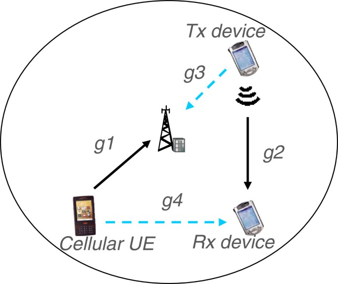

  

  Illustration of the useful path loss links (g1 and g2) and the interference path loss links (g3 and g4) in a cell that form the inputs of the heuristic MS algorithm under study..

• $g_{{\mathrm{RxD}}_l,{\mathrm{TxD}}_l}=d_{{\mathrm{RxD}}_l,{\mathrm{TxD}}_l}^{-\rho }·{\chi }_{{\mathrm{RxD}}_l,{\mathrm{TxD}}_l}$: Large scale fading between the D2D transmitter and receiver of Cell-l (see g2 link in Figure 5);

• $g_{{\mathrm{BS}}_l,{\mathrm{TxD}}_l}=d_{{\mathrm{BS}}_l,{\mathrm{TxD}}_l}^{-\rho }·{\chi }_{{\mathrm{BS}}_l,{\mathrm{TxD}}_l}$: Large scale fading between the D2D transmitter and the BS of Cell-l (see g3 link in Figure 5);

• $g_{{\mathrm{RxD}}_l,{\mathrm{CellUE}}_l}=d_{{\mathrm{RxD}}_l,{\mathrm{CellUE}}_l}^{-\rho }·{\chi }_{{\mathrm{RxD}}_l,{\mathrm{CellUE}}_l}$: Large scale fading between the cellular UE and the D2D receiver of Cell-l (see g4 link in Figure 5).

The fourth requirement implies that the MS algorithm should rely on SNR rather than SINR metrics, since the measured SINR at the receivers (D2D receiver or cellular BS) depend on the transmit powers of the interferers (see also our proposed SNR metric in Algorithm 3). Finally we note that the proposed MS algorithm does not consider the hop gain that is described in the Introduction of this article. That is, the MS algorithm is somewhat biased towards favoring the cellular mode, since it disregards the potential hop gain of the D2D mode. Based on these requirements, in this article we propose a simple MS algorithm described by Algorithm 3.

Algorithm 3 Simple MS algorithm based on single-cell knowledge

Input: $\Delta ,\rho ,{\sigma }_n^2,p=p_{\max }$, number of cells (L), and $g_{k,j}=d_{k,j}^{-\rho }{\chi }_{k,j}$, k = 1,…,K,j = 1,…,J, as in Equation (1) where K and J are the number of receivers and transmitters, respectively.

Output: Decision on which mode is preferred (D2D or Cellular) for all cells:

useD2D _l ∈{True,False}, l=1,…,L.

Notations:

BS _l - the cellular BS of cell l

CellUE _l - the cellular UE in cell l

RxD _l - the D2D receiver in cell l

TxD _l - the D2D transmitter in cell l

for l = 1 to L do

• 1. The useful (u) signal path loss in Cellular (C) mode is $g_{{\mathrm{BS}}_l,{\mathrm{CellUE}}_l}$, hypothetical SNR

  $${\gamma }_l^{u,\mathrm{C}}=\frac{p·g_{{\mathrm{BS}}_l,{\mathrm{CellUE}}_l}}{{\sigma }_n^2};$$

• 2. The useful signal path loss in D2D mode is $g_{{\mathrm{RxD}}_l,{\mathrm{TxD}}_l}$, hypothetical SNR

  $${\gamma }_l^{u,\mathrm{D}2D}=\frac{p·g_{{\mathrm{RxD}}_l,{\mathrm{TxD}}_l}}{{\sigma }_n^2};$$

• 3. The interfering (i) signal path loss in Cellular mode is $g_{{\mathrm{BS}}_l,{\mathrm{TxD}}_l}$, hypothetical SNR

  $${\gamma }_l^{i,\mathrm{C}}=\frac{p·g_{{\mathrm{BS}}_l,{\mathrm{TxD}}_l}}{{\sigma }_n^2};$$

• 4. The interfering signal path loss in D2D mode is $g_{{\mathrm{RxD}}_l,{\mathrm{CellUE}}_l}$, hypothetical SNR

  $$\begin{array}{lcr}{\gamma }_l^{i,\mathrm{D}2D}& =& \frac{p·g_{{\mathrm{RxD}}_l,{\mathrm{CellUE}}_l}}{{\sigma }_n^2};\end{array}$$

• 5. Select whether Cellular or D2D mode is beneficial to use as:

if $\left(\underset{2}{log}\right(1+{\gamma }_l^{u,\mathrm{D}2D})+\underset{2}{log}(1+{\gamma }_l^{u,\mathrm{C}})-\underset{2}{log}(1+{\gamma }_l^{i,\mathrm{D}2D})-\underset{2}{log}(1+{\gamma }_l^{i,\mathrm{C}})>\Delta )$ then

useD2D _l =True

else useD2D _l =False;

end

The proposed algorithm is based on the geometry of the UEs in the own cell, i.e., the geometry situations in the neighbor cells are not considered. Figure 5 illustrates the idea of Algorithm 3, where the useful and the interference path loss links are shown for a particular D2D candidate pair and a cellular UE in a specific Monte Carlo drop. The useful path loss links are denoted with bold black arrows (g1 and g2), while the interference path loss links (g3 and g4) are marked with dashed blue arrows. The algorithm first calculates hypothetical SNR values for each link according to Step 1–4. The proposed algorithm selects D2D mode for the D2D candidate if the useful links (g1 and g2) are stronger than the interfering links (g3 and g4). More specifically, D2D mode is selected if the hypothetical capacity values corresponding to the useful links are higher than the hypothetical capacity values corresponding to the interfering links plus a Δ value (see Step 5 of Algorithm 3), which is a tunable system parameter measured in bit/sec/Hz. The transmit power value p in Step 1)– 4) is set to an arbitrary positive value. By increasing Δ, the MS algorithm becomes more conservative and selects D2D communication more cautiously. Selecting a negative Δ implies a more frequent D2D MS. This algorithm is not a network-wise optimization in the sense that it uses only single cell slow fading (distance dependent path loss and shadowing) information to determine the communication mode of a cell. An important feature of this algorithm is that it meets Requirement 4 by relying on SNR rather than SINR metrics.

Numerical results

In this section we first discuss how the proposed algorithms can be deployed and executed in a real network. Then, we examine a 2-cell system (that primarily serves the purpose of benchmarking the target setting heuristic) and a 7-cell system that more realistically represents a multicell system. In the following, we use the solution of the optimization problem of Section “The problem of optimal SINR target selection” as a reference case which uses full channel knowledge including fast fading (Rayleigh) information. In each simulation scenario, Algorithm 1 is used to adjust the power values where some fast fading knowledge (total received interference and noise covariance) is also exploited as detailed in Section “An iterative D2D power control scheme”. In numerical results based on Algorithms 2 and 3, only slow scale fading (distance dependent pathloss and shadowing) information is considered as also stated in Sections “Determining the optimum SINR target” and “Mode selection”, respectively (see Table 2 for the values of the simulation parameters).

Table 2 The input parameters used in the simulations

System operation

In a practical system, the proposed distributed power control scheme, the adaptive SINR target setting and the model selection algorithms should be executed in the following order.

• 1. Run the MS algorithm (Algorithm 3) in each cell to select between the cellular and D2D communication modes (i.e, to select the links for transmission) on the time scale of few hundred milliseconds based on large scale fading (distance dependent path loss and shadowing) information of the own cell.

• 2. Execute the adaptive SINR target setting algorithm (Algorithm 2) on the transmission links (selected by MS) to minimize the sum transmit power. The time scale is the same as that of the MS.

• 3. Run the distributed power control scheme (Algorithm 1) to set the transmit power for each link in each transmission slot taking into account fast fading information as well.

The above operation of the system is reasonable, since MS should decide first which links are going to transmit in the next few transmission slots. As discussed, for instance, in [28], the time scale of MS should match that of handover and should rely on large scale fading information only (see also the requirements in Section “Mode selection”). The execution of the SINR target setting algorithm is optional, though significant power can be saved by tuning the SINR target according to the large scale channel conditions while maintaining some fairness criterion as well (see the numerical results of Sections “2-cell system results” and “7-cell system results”). Finally, the proposed distributed power control scheme combats against fast fading by measuring the covariance of the total received interference and noise in each transmission slot.

2-cell system results

We consider two sets of numerical results. The first set focuses on the performance of Algorithm 1 given a fixed set of SINR targets. The second set shows the gains when setting the SINR targets in an optimal or heuristic fashion.

Simulation scenarios

We consider two simulation scenarios as shown in Figure 6 (Scenarios 1 and 2 are illustrated on the left and right part of Figure 6, respectively), which are basically two instances of the scenario shown in Figure 1. In Scenario 1 the D2D pair is randomly dropped in an area that is “on the other side” of the access point than UE1. In Scenario 2, the D2D pair is randomly dropped in an area close to UE1. In both scenarios, UE1 moves from the cell center to the cell edge (Position 1 …Position 10). UE2 is the transmitting UE of the D2D pair. UE3 is a stationary interfering UE at a fixed position in the neighbor cell. We denote with UE1 the UE transmitting to its serving BS. We let UE1 move from a position close to the BS (UE1 Position 1) towards the cell edge (UE1 Position 10). We use the UE1 position along the x axis of all our plots. UE2 denotes the transmitting UE (Tx UE) of the D2D pair. Finally, UE3 denotes an interfering UE at a fixed position in a neighbor cell served by access point AP2. The D2D pair is dropped within the half circle areas denoted in Figure 6 in 40000 Monte Carlo experiments.

Figure 6

2-cell simulation scenarios. In Scenario 1 (left) the D2D pair is randomly dropped in an area that is “on the other side” of the access point than UE1. In Scenario 2, the D2D pair is randomly dropped in an area close to UE1. In both scenarios, UE1 moves from the cell center to the cell edge (Position 1 …Position 10). UE2 is the transmitting UE of the D2D pair. UE3 is a stationary interfering UE at a fixed position in the neighbor cell.

The D2D pair can communicate in two modes:

• 1. D2D mode: The two UEs of the D2D pair communicate via a direct link. In this mode, the D2D link uses the same OFDM resource blocks as the UE1 uses to communicate with its serving AP.

• 2. Cellular mode: The two UEs of the D2D pair communicate via the serving AP. In this case the UE1 and UE2 use orthogonal uplink resources (either in the time or in the frequency domain). For example, assuming a time domain separation, during the first period only UE1 transmits to AP1 followed by a period when only UE2 transmits to AP1. (The resources are split equally between UE1 and UE2).

The two performance measures of interest are the sum power for a given sum capacity target (UE1 + UE 2 + UE 3) and the probability that the (fixed or set) SINR targets are infeasible. Some of the simulation parameters are listed in Table 2. Recall that for the SINR target optimization, fast fading is taken into account in the reference (centralized) case, whereas only distance dependent path loss and shadowing are considered in the distributed approach.

Results for predefined SINR targets

Figures 7 and 8 present results for the fixed SINR target case and compare the performance of D2D mode and cellular mode between the D2D pair in terms of the performance measures of interest. The SINR target for D2D mode is set to ${\gamma }_{D2D}^{\mathrm{tgt}}=4\mathrm{dB}$ for all three links (UE1, UE2 and UE3). For the cellular mode, the SINR target is set such that the total capacity be the same as in the D2D mode. Since in cellular mode there is only one communication link (apart from the interfering neighbor, UE3) at a time, the SINR target is set such that $3·\underset{2}{log}({\gamma }_{D2D}^{\mathrm{tgt}}+1)=2·\underset{2}{log}({\gamma }_{\mathrm{Cell}}^{\mathrm{tgt}}+1)$ (that is: ${\gamma }_{\mathrm{Cell}}^{\mathrm{tgt}}=7.47\mathrm{dB}$).

Figure 7

Sum power and infeasibility in Scenario 1 (1 × 2 SIMO). Required sum power and probability of infeasibility are shown with fixed SINR targets (1 × 2 SIMO) in Scenario 1. When the D2D pair communicates in D2D mode, the average sum power is significantly lower than the average sum power in cellular mode. This SINR target is also more often feasible in D2D mode than in cellular mode.

Figure 8

Sum power and infeasibility in Scenario 1 (2 × 4 MIMO). Required sum power and probability of infeasibility are illustrated with fixed SINR targets (2 × 4 MIMO) in Scenario 1. This figure is similar to Figure 7. In this case the SINR targets are typically not feasible except when the UE1 is in the cell center.

The upper graph of Figure 7 shows the sum power results for the 1 × 2 SIMO case. As UE1 moves from its cell center position towards the cell edge, the average sum power (on the three links) required to reach their respective SINR targets gradually increases both when the D2D pair communicates in D2D mode and when they communicate in cellular mode. Recall that in cellular mode, we first assume that only UE1 transmits and then only UE2 transmits to the AP (when only UE2 transmits, the required power is obviously independent from the UE1 position, since UE1 does not transmit). What is important to notice here is that the sum power is always lower (roughly 30% of the average power used in cellular mode) in the D2D mode than in cellular mode due to the reuse and proximity gains in D2D mode.

The lower graph of Figure 7 shows the probability that in a Monte Carlo experiment the SINR targets are infeasible. As expected, the probability of infeasibility increases as UE1 moves towards the cell edge, but this probability is significantly lower (typically half or less) in D2D mode.

In Figure 9, we show the sum power and infeasibility results in Scenario 1, but the stationary interfering UE (UE3) connected to AP2 is placed only to radius/2 distance from the cell center (in the same angle as in Scenario 1), i.e., UE1 and UE3 are farther from each other. In this case, the sum power and infeasibility ratio are considerably lower than in Figure 7, since UEs in both cells generate lower interference to UE(s) in the neighbor cell, because (1) they are geographically farther from each other, i.e., signals experience higher attenuation at the neighbor receiver and (2) the UEs can transmit with reduced power to achieve the required SINR target.

Figure 9

Sum power and infeasibility in Scenario 1 (1 × 2 SIMO) when UE3 is closer to cell center. Required sum power and probability of infeasibility are shown with fixed SINR targets (1 × 2 SIMO) in Scenario 1 when the stationary interfering UE (UE3) is moved only to half-radius distance from the cell center (in the same angle as in Scenario 1). The sum power and infeasibility ratio is lower compared to Figure 7, since the sum interference is reduced in the system.

Figure 8 shows the sum power and the probability of infeasibility in Scenario 1 for the 2 × 4 MIMO case and setting the SINR target per stream to 4 dB (that is setting the sum capacity target to twice of that required in Figure 7). This high SINR per stream target is basically only feasible when UE1 is in the cell center. Similarly to the 1 × 2 case, the D2D mode between UE2 and its D2D pair is clearly superior to the cellular mode both in terms of sum power and feasibility.

Results for optimal and heuristic SINR targets

We discuss the results when the SINR targets are not fixed, but set optimally or by means of the proposed heuristic SINR target setting algorithm such that the sum rate capacity is the same as in the fixed SINR target case of the previous section (that is 5.44 bps/Hz in the 1 × 2 SIMO case and 2 × 5.44 bps/Hz in the 2 × 4 MIMO case).

First, we consider the results for the 1 × 2 SIMO case (Figure 10) in Scenario 1. In this case, the required sum power is drastically lower than in the fixed SINR target case. For example, when UE1 is at the cell edge, the required sum power in D2D mode is only around 30 mW (with optimal SINR targets) and around 40 mW (with heuristic SINR targets) as compared to 125 mW with the fixed SINR targets (of Figure 7). We also notice that virtually all drops turn out to be feasible, both with optimal SINR targets and with the proposed SINR target setting algorithm.

Figure 10

D2D sum power and infeasibility in Scenario 1 (1 × 2 SIMO). Performance measures of interest are shown in D2D mode with optimized and heuristically set SINR targets (1 × 2 SIMO) in Scenario 1. The target sum rate is the same as in Figure 7, but the required sum power is just a fraction of that with fixed SINR targets (see Figure 7). In addition, the probability of infeasibility is very low, even when UE1 approaches the cell edge.

The results for the 2 × 4 MIMO case without and with power loading are shown in Figures 11 and 12, respectively. The lower graph of Figure 12 illustrates the average sum power results in Scenario 2 (see the right part of Figure 6). As expected, this scenario requires somewhat higher average sum power than Scenario 1, since the transmitting UEs are closer to each other, and thereby, the interference is higher in the system.

Figure 11

D2D sum power and infeasibility in Scenario 1 (2 × 4 MIMO). Performance measures of interest are shown in D2D mode with optimized and heuristically set SINR targets (2 × 4 MIMO) without power loading optimization in Scenario 1. Compared with the results of Figure 8, we notice the dramatic decrease in the required power and the improved feasibility probability. Except for the UE1 cell edge positions, the same sum rate that is typically infeasible with fixed SINR targets becomes typically feasible with proper SINR target setting.

Figure 12

D2D sum power with power loading in Scenario 1 and 2 (2 × 4 MIMO). Average sum power is illustrated in D2D mode with optimized and heuristically set SINR targets (2 × 4 MIMO) and with power loading optimization in Scenario 1 (upper) and Scenario 2 (lower). Power loading helps further reduce the required power to reach the sum rate target (the feasibility probability is roughly the same as without power loading (Figure 11) in both scenarios.) In Scenario 2, the average sum power is increased since UE1 and UE3 are closer to Rx UE and thus, the received interference is higher than in Scenario 1.

Recall from Figure 8 that in this case the fixed SINR targets were typically infeasible. With optimal and heuristic SINR targets, the same sum rate becomes feasible except when UE1 is close to the cell edge. Also the sum power in the feasible drops becomes only a fraction of what is required in the fixed SINR case.

In both the 1 × 2 SIMO and the 2 × 4 MIMO case we also notice that D2D mode provides better performance than cellular mode.

7-cell system results

In this section we consider a 7-cell system as shown in Figure 13 (Scenario 3), where a D2D candidate pair and a cellular UE are dropped in each cell according to a surface uniform distribution in a series of Monte Carlo experiments. The dropping of the cellular UEs and the D2D pairs is independent from each other.

Figure 13

7-cell simulation scenario. Scenario 3 is a 7-cell system used for illustrating the performance aspects of D2D communications. The D2D receiver and transmitter in each cell is marked with red square and red rhombus, respectively, while the UE communicating with the cellular BS is denoted by black triangle. The BS is marked with a grey square. The figure shows an instance of a series of Monte Carlo simulations.

In this network, when all D2D candidates transmit directly, i.e., in D2D mode there are 14 simultaneous transmissions. In this case, we set the fixed SINR target for all links to 2 dB resulting in 19.18 b/s/Hz spectral efficiency. When each cell communicates in cellular mode, we have seven simultaneous transmissions in the whole system and the fix SINR target is set to 7.54 dB in order to achieve exactly the same sum capacity as with pure D2D mode.

Recall from Section “Mode selection”, that we assume that there are at most two links (one cellular and one D2D) multiplexed on a single OFDM resource block. Therefore, just like e.g. [36], we focus on a single resource block (used by at most 3 users), since each resource block of the system bandwidth can be studied in isolation.

Potential of D2D communication

To get insight into the potential of D2D communication, we illustrate the performance measures of interest in Scenario 3 using 1 × 2 SIMO system as shown in Figure 14. The green surface shows the system performance in the D2D mode with fixed SINR targets, while the blue one uses the cellular mode when also fixed SINR targets are set in the system. In D2D mode, the required sum power is sensitive not only to the D2D distance, but also to the position of the cellular UE with which the D2D candidate reuses the PRB. We see that the system performance for up to 100 m maximum D2D distance, and especially when the cellular UE is close to the cell center is significantly better in D2D mode, both in terms of sum power and infeasibility probability.

Figure 14

Potential of D2D communications with fixed SINR targets. Average sum power and infeasibility probability are shown in Scenario 3 (7-cell system) using fixed SINR targets. When D2D candidates use D2D mode, the gain of D2D communications heavily depends on the maximum D2D distance and also on the position of the cellular UE with which the D2D link shares the cellular resources (uplink PRB).

In Figure 15, the we illustrate the system performance when using the proposed adaptive SINR target setting algorithm. As we see in the figure, adaptive SINR targets lead to a significant improvement both in D2D and cellular modes both in terms of sum power and infeasibility probability. The reason for this is that the adaptive SINR target setting algorithm sets a higher SINR target for links with a low path loss value thereby the algorithm encourages allocating power on links with a high rate utility. More interestingly, D2D mode shows superior performance even when the D2D distance is high and for all cellular UE positions. The reason for this improvement is that adaptive SINR targets are the key to fully exploit the proximity gain and at the same time control the interference between the D2D and the cellular layer.

Figure 15

Potential of D2D with adaptive SINR targets. Average sum power and infeasibility probability are shown in Scenario 3 (7-cell system) using adaptive SINR targets. When the SINR targets are properly set, D2D communications has the potential to drastically reduce the average sum power as well as the probability of infeasibility over a wide range of D2D distances and cellular UE positions.

Numerical results with MS

As shown in Figures 14 and 15, the benefit of the D2D communications much depends on the geometry of the UEs sharing the same resource block, which also indicates the need for the MS mechanism. We evaluate our proposed MS algorithm described in Section “Mode selection” and present the results in Figure 16 where four other cases are compared to the performance of the MS algorithm.

Figure 16

Comparisons of performance results with maximum D2D distance of ISD/5. Comparisons of the average sum power and infeasibility ratio are illustrated in different cases when the D2D pair is dropped within ISD/5 distance from one another in Scenario 3 (7-cell system). When a minimum SINR target is required (denoted with “+F”, F indicating fairness), adaptive SINR target setting with MS provides superior performance. The average sum power is of course much lower when no minimum SINR is required (“lowest” curve).

The upper plot of Figure 16 compares the average sum power in different cases in Scenario 3 when we use a 1 × 2 SIMO system and the D2D pair is dropped at most 100 m far away from each other (within one fifth of the ISD). The blue curve (“Cellular-Fixed SINR”) shows the system performance in Cellular mode, which can serve as a reference, since this curve corresponds to the currently deployed systems. When we apply D2D mode for the D2D candidates we obtain the dark red curve (“D2D-Fixed SINR”). We can see that there is significant gain compared to the Cellular mode when the cellular UE is close to the cellular BS. The gain is decreasing as the cellular UE moves toward the cell edge. If we use the heuristic SINR target settings in D2D mode (yellow curve with rhombus symbols), we can observe that employing adaptive SINR targets in D2D mode provides very low sum power. This large sum power reduction comes at the price of setting very low SINR targets for some of the links, sometimes allocating close to zero power for some links as we will show later in Figures 17 and 18. This issue can be solved by setting a minimum SINR in the heuristic SINR target setting algorithm in order to avoid the cases when some links are in outage. An example for this is also shown in Figure 16 by the green curve (“D2D − adaptive SINR + F”) when the minimum SINR is set to 1 dB for all links in D2D mode with adaptive SINR targets. It still brings significant gain compared to the fixed SINR targets (dark red curve).

Figure 17

The empirical CDF of the received SINR is illustrated when operating in D2D mode and the D2D pair is dropped within ISD/5 distance from one another in Scenario 3 (7-cell system). The plot verifies that the fixed SINR target is maintained for all UEs in the cell (i.e. both the cellular UEs and the receiving device (RxD) of the D2D pair). The heuristic (adaptive) SINR targets are set such that SINR target on the D2D link (RxD) has a wide range of possible values throughout the Monte Carlo experiments, while the SINR targets for the cellular UEs are typically very low (essentially switching off the cellular link).

Figure 18

The empirical CDF of the per UE transmit power is shown when adaptive SINR target setting is used with minimum SINR of −10 dB and the D2D pair is dropped within ISD/5 distance from each other in Scenario 3 (7-cell system). The adaptive SINR setting algorithm allocates very low transmit power values to the cellular UE, therefore it achieves very low SINR also as shown in Figure 17.

The performance result of the MS algorithm together with 1 dB minimum SINR is shown by the light blue color (“Mode selection− adaptive SINR + F”). As it can be seen, the employment of MS gives some additional gains to D2D mode with minimum SINR. This gain comes from that that the MS algorithm avoids using D2D mode in such cases when, for example, a cellular UE is placed very close to a D2D receiver and would suppress the transmission of the D2D transmitter. In Figure 16, it is clearly visible that MS combined with adaptive SINR target setting can provide superior performance, even when a minimum SINR target is required on all links.

Looking at the lower plot of Figure 16, we can observe that the infeasibility probability is in line with the result of the average sum power results of the upper plot. These results highlight the importance of MS combined with adaptive SINR target setting.

Figure 19 shows the probability that D2D mode is selected by the MS algorithm when the maximum D2D distance is limited to 100 m in the function of the cellular UE position. As expected, as the cellular UE is placed closer to the cell edge, the MS algorithm tends to select the cellular mode for the D2D candidate, but it is noteworthy that even in UE position 10, in 80% of the experiments, D2D mode is preferred for the D2D candidate since the maximum D2D distance is bounded and thus the link between the D2D candidate pair (g2) is “almost always” better than the interference links (g3 and g4). The remaining 20% of the drops cover such cases when e.g., the cellular UE is placed very close to the D2D receiver and would suppress the transmission of the D2D transmitter.

Figure 19

The probability that D2D mode is selected by the MS algorithm is shown when the maximum D2D distance is limited to 100 m (ISD/5) in Scenario 3 (7-cell system).

The gain of the MS algorithm comes from the fact that it avoids using D2D mode in cases when the transmission of one layer (D2D or cellular) would be suppressed due to the proximity of the receiver of the other layer. This algorithm can be thought of as an additional sanity check to adapt to realistic situations and avoid using simultaneous transmissions within a cell, i.e., D2D mode when high intra-cell interference can be expected.

Figure 17, presents empirical cumulative distribution functions (CDF) of the received SINR in different cases in Cell-1, which is the cell in the middle among the seven cells. In this figure the D2D candidate operates in D2D mode. This cell is in the worst situation, since it receives the most interference from the neighbors. We use a 1   2 SIMO system where the maximum D2D distance is also limited to 100 m. We focus on the cellular UE position 5, i.e., when the cellular UE is around the same distance from the BS as from the cell edge. We compare four different cases, where the black curve shows the CDF of the received SINR at the receiver device of the D2D pair when fixed SINR targets are set and D2D mode is used in the cell (Cell-1). The reason why it is hard to distinguish the black curve (“RxD-fixed SINR-D2D”) is that all points are at exactly 2 dB as expected, verifying that the power setting algorithm (Algorithm 1) works well. The result is similar to the SINR at the cellular BS (red curve), since 2 dB target SINR is set for the cellular UE as well. The next two curves (green and blue) show the same results when employing adaptive SINR targets (“RxD-Adaptive SINR-D2D”, “Cellular BS-Adaptive SINR D2D”). In this case, we set the minimum SINR to −10 dB. The SINR of the receiver device can be in very wide range from −10 to 30 dB as shown by the green curve, which also confirms that it is hard to set one single SINR target that is optimal or “good enough” for both D2D and cellular modes. The problem of adaptive SINR target is illustrated by the blue curve of Figure 17 (“Cellular BS-Adaptive SINR D2D”) where in the 90% of the cases, the SINR at the cellular BS is around or below −10 dB. This means that the algorithm puts this link into outage. There is a need to introduce the concept of the minimum SINR to avoid situations in which one of the transmission links is practically muted.

The CDFs of the UE transmit power are plotted in Figure 18. We conclude that the cellular UE (red curve) consumes the most power to reach the 2 dB fixed SINR target. This can be expected, since this UE is in cellular UE position 5, which is around 125 m far from its serving BS, but the D2D pair is placed at most 100 m from each other. In Figure 20, the same empirical CDF curves are plotted as in Figure 17 when the minimum SINR is set to 1 dB in order to avoid causing outage. As it can be observed, all of the SINR values are above 1 dB and for the fixed cases (black and red curves) the SINR is exactly 2 dB (“RxD-Fixed SINR-D2D” and “Cell BS-Fixed SINR D2D”). It is important to notice that when the SINR targets are set adaptively, the D2D receiver can experience more than 2 dB SINR (green curve, “RxD-Adaptive SINR-D2D”) in about the 20% of the cases which provides the gain of adaptive SINR target setting together with minimum SINR compared to the predefined SINR target case, which causes a significant performance difference (both in terms of average sum power and infeasibility) between these two cases shown by the red and green curves of Figure 16.

Figure 20

The empirical CDF of the received SINR is illustrated when adaptive SINR target setting is used with a minimum SINR of 1 dB and the D2D pair is dropped within ISD/5 distance from one another in Scenario 3 (7-cell system). The figure verifies that the minimum SINR target setting guarantees a received SINR value (1 dB). Also, when using the adaptive SINR target setting algorithm, the D2D link SINR target can be set to significantly higher values.

Figure 21 shows the UE transmit power CDF curves when the minimum SINR is set to 1 dB. The power of the cellular UE is increased significantly when adaptive SINR target setting is used since it needs to increase the transmit power to improve its SINR to 1 dB. It is interesting to note that the power consumptions of the cellular UE contribute the most to the average sum power, which has a consequence that if we further reduce the maximum D2D distance, we cannot expect significant reduction in the average sum power. This can be verified by comparing Figure 16 with Figure 22 in which the maximum D2D distance is limited to 25 m (ISD/20).

Figure 21

The empirical CDF of the per UE transmit power is shown when adaptive SINR target setting is used with minimum SINR of 1 dB and the D2D pair is dropped within ISD/5 distance from each other in Scenario 3 (7-cell system). The figure shows that the cellular UE is the main contributor of the power consumption with both the fixed and the adaptive SINR targets.

Figure 22

Comparison of the average sum power is shown in different cases when the D2D pair is dropped within ISD/20 distance from one another in Scenario 3 (7-cell system). Comparing these results to that of Figure 16 with maximum D2D distance of ISD/5, the average sum power is not reduced significantly, since the cellular UE is the dominant contributor to the sum power consumption.

Computational complexity of the distributed SINR target setting algorithm

Algorithm 2 scales linearly in the number of transmissions, because Step 1) of Algorithm 2 (for loop) runs exactly as many times as the number of simultaneous transmissions in the whole system, e.g., in a 7-cell OFDM system, Step 1) runs 7 times in cellular and 14 times in D2D mode. The number of iterations (t) in Algorithm 2 depends on the values of parameter Δ by which the SINR is increased in each iteration and parameter C^sum. When C^sum is fixed and Δ is set to a higher value (e.g., 1–2 dB), the convergence is faster (see the left graph of Figure 23) but more inaccurate, since the sum capacity target is overshot by at most log₂(1 + Δ) bit/s/Hz resulting in higher sum power consumption as illustrated in the middle graph of Figure 23. The number of iterations is also sensitive to the value of SINR^min, because the higher the value of this parameter the higher the achieved sum capacity in the beginning of the execution, thus less capacity different must be worked off in the remaining iterations. The number of required iterations linearly decreases in the function of the minimum SINR (in logarithmic scale). More specifically, the reduction in the number of iterations equals the change in the minimum SINR required multiplied by the number of simultaneous transmissions as also confirmed by the right graph of Figure 23. For example, when SINR^min=2 dB, the number of iterations is 38, while with SINR^min=4 dB, it reduces to 24, i.e., the difference in the number of iterations equals 14=(4−2 dB)·7 simultaneous transmissions. We note that ${\gamma }_k^{\left(0\right)}$ in Algorithm 2 is set to the minimum SINR (SINR^min) required for all links (i.e., ∀k) and the initial power levels are calculated accordingly.

Figure 23

Computational complexity of Algorithm 2. The average number of iterations (left), the average sum power (middle) in the function of Δ, and the average number of iterations in the function of SINR^min(right) are shown in Algorithm 2 when the minimum SINR (SINR^min) is set to 1 dB and C^sum=19.18b/s/Hz in Scenario 3 (7-cell system) using cellular mode. The required number of iterations decreases exponentially as Δ(in logarithmic scale) increases (left). With higher Δ values, the sum capacity target is exceeded and the used sum power slightly increases, which means that the accuracy of the algorithm (in terms of keeping the sum rate target) somewhat decreases (middle). The number of iterations reduces linearly in the function of the required minimum SINR in logarithmic scale (right).

Conclusions

In this article we developed a distributed power control and MS algorithm for cellular network assisted D2D communications. The power control algorithm consists of an SINR target setting part that aims to set the individual SINR targets such that the required sum power is minimized with respect to a sum rate target and a power allocation part that sets the power levels and power loading matrices over multiple MIMO streams. The MS algorithm considers the geometry of the D2D candidate and the cellular UE communicating with the cellular access point and determines if the D2D candidate should use the direct D2D link or should communicate via the cellular access point.

Numerical results clearly indicate that in order to take advantage of the proximity and reuse gains of D2D communications, adaptively setting the SINR targets for both the cellular and D2D links and adaptively determining the communication mode for the D2D candidate are necessary. To this end, we proposed low complexity power control and MS algorithms that rely on slow scale CSI. When the proposed power control and MS algorithms are employed, D2D communication is clearly superior both in terms of the required sum power and the feasibility of a predefined sum rate target to the classical cellular mode of operation.

The numerical examples also suggest that due to the combination of the intra- and intercell interference, it becomes important that the power control algorithm ensures some level of fairness between the D2D and the cellular links. The proposed power control algorithm is therefore capable of guaranteeing a predefined minimum SINR target to each link. This feature of the power control algorithm along with the low complexity of the MS algorithm make them interesting candidates for future networks supporting D2D communications.

Endnotes

^aThis article is a substantially revised and extended version of the article “A Distributed Power Control Scheme for Cellular Network Assisted D2D Communications” presented at the IEEE Global Communication Conference (Globecom), in Houston, TX, USA, December 2011 [30].^bIt is advantageous to use uplink resources for the D2D link, because in some countries regulatory requirements may not allow to use downlink resources by UEs in the future. Therefore, in this article we only deal with the case when the D2D links use UL cellular resources, such as the uplink OFDM resource blocks in a cellular Frequency Division Duplexing system or the uplink time slots in a TDD system [28, 40, 41].

Appendices

Appendix 1: derivation of the MMSE estimation error matrix

By applying the standard theory on linear MMSE computation to the model see e.g. ([37], Chapter 12), the MMSE error covariance matrix for the k th receiver is

$$\begin{array}{ll}{\mathbf{E}}_k& =\mathbb{E}\left[({\hat{\mathbf{x}}}_k-{\mathbf{x}}_k){({\hat{\mathbf{x}}}_k-{\mathbf{x}}_k)}^{†}\right]=\\ ={\alpha }_{k,k}^2{\mathbf{G}}_k{\mathbf{H}}_{k,k}{\mathbf{T}}_k{\mathbf{T}}_k^{†}{\mathbf{H}}_{k,k}^{†}{\mathbf{G}}_k^{†}-2{\alpha }_{k,k}{\mathbf{G}}_k{\mathbf{H}}_{k,k}{\mathbf{T}}_k+\\ +{\mathbf{G}}_k{\mathbf{R}}_{z_k}{\mathbf{G}}_k^{†}+{\mathbf{G}}_k{\mathbf{R}}_{n_k}{\mathbf{G}}_k^{†}=\\ =({\alpha }_{k,k}{\mathbf{G}}_k{\mathbf{H}}_{k,k}{\mathbf{T}}_k-\mathbf{I})({\alpha }_{k,k}{\mathbf{T}}_k^{†}{\mathbf{H}}_{k,k}^{†}{\mathbf{G}}_k^{†}-\mathbf{I})+{\mathbf{G}}_k{\mathbf{R}}_{v_k}{\mathbf{G}}_k^{†}.\end{array}$$

Finally, by replacing the expression of G _k into E _k and using similar techniques as in [35] we obtain

$$\begin{array}{ll}{\mathbf{E}}_k& =\mathbf{I}-{\alpha }_{k,k}{\mathbf{T}}_k^{†}{\mathbf{H}}_{k,k}^{†}·\\ ·{\left({\alpha }_{k,k}^2{\mathbf{H}}_{k,k}{\mathbf{T}}_k{\mathbf{T}}_k^{†}{\mathbf{H}}_{k,k}^{†}+{\mathbf{R}}_{v_k}\right)}^{-1}{\alpha }_{k,k}{\mathbf{H}}_{k,k}{\mathbf{T}}_k=\\ ={(I+{\mathbf{T}}_k^{†}{\mathbf{R}}_{H_k}{\mathbf{T}}_k)}^{-1},\end{array}$$

where ${\mathbf{R}}_{H_k}={\alpha }_{k,k}^2{\mathbf{H}}_{k,k}^{†}{\mathbf{R}}_{v_k}^{-1}{\mathbf{H}}_{k,k}$.

Appendix 2: derivation of Δ P in Algorithm 2

Derivation of Δ P in Algorithm 2:

$$\begin{array}{ll}{\gamma }_k^{\left(t\right)}& \approx \frac{p_k^{\left(t\right)}{g}_{k,k}}{\sum _{j\ne k}^J{p}_j^{(t-1)}{g}_{k,j}+{\sigma }_n^2}\\ p_k^{\left(t\right)}& \approx \frac{{\gamma }_k^{\left(t\right)}\left(\sum _{j\ne k}^J{p}_j^{(t-1)}{g}_{k,j}+{\sigma }_n^2\right)}{g_{k,k}}\end{array}$$

(27)

$$\begin{array}{ll}{\gamma }_k^{\left(t\right)}\Delta & \approx \frac{p_k^{\left(t\right)\prime }{g}_{k,k}}{\sum _{j\ne k}^J{p}_j^{(t-1)}{g}_{k,j}+{\sigma }_n^2}\\ p_k^{\left(t\right)\prime }& \approx \frac{{\gamma }_k^{\left(t\right)}\Delta \left(\sum _{j\ne k}^J{p}_j^{(t-1)}{g}_{k,j}+{\sigma }_n^2\right)}{g_{k,k}}\end{array}$$

(28)

The approximated transmission power needed to increase the SINR by Δ can be calculated from (27) and (28) as ${\mathrm{\Delta P}}_k^{\left(t\right)}=p_k^{\left(t\right)\prime }-p_k^{\left(t\right)}$.

Appendix 3: components of the sum power vector

The parameters introduced in (25) are as follows:

$$\begin{array}{ll}{M}_{1,1}& =a_1\kappa {\gamma }_1^{\mathrm{tgt}}\left(F_{1,3}+{\gamma }_2^{\mathrm{tgt}}{F}_{1,2}{F}_{2,3}\right),\\ M_{1,2}& =a_2{\gamma }_1^{\mathrm{tgt}}{\gamma }_2^{\mathrm{tgt}}\left(F_{1,2}+\kappa F_{1,3}{F}_{3,2}\right),\\ M_{1,3}& =a_3{\gamma }_1^{\mathrm{tgt}}\left(1-\kappa {\gamma }_2^{\mathrm{tgt}}{F}_{2,3}{F}_{3,2}\right),\\ M_{2,1}& =a_1\kappa {\gamma }_2^{\mathrm{tgt}}\left(F_{2,3}+{\gamma }_1^{\mathrm{tgt}}{F}_{1,3}{F}_{2,1}\right),\\ M_{2,2}& =a_2{\gamma }_2^{\mathrm{tgt}}\left(1-\kappa {\gamma }_1^{\mathrm{tgt}}{F}_{1,3}{F}_{3,1}\right),\\ M_{2,3}& =a_3{\gamma }_1^{\mathrm{tgt}}{\gamma }_2^{\mathrm{tgt}}\left(F_{2,1}+\kappa F_{2,3}{F}_{3,1}\right),\\ M_{3,1}& =a_1\kappa \left(1-{\gamma }_1^{\mathrm{tgt}}{\gamma }_2^{\mathrm{tgt}}{F}_{1,2}{F}_{2,1}\right),\\ M_{3,2}& =a_2{\gamma }_2^{\mathrm{tgt}}\kappa \left(F_{3,2}+{\gamma }_1^{\mathrm{tgt}}{F}_{1,2}{F}_{3,1}\right),\\ M_{3,3}& =a_3\kappa {\gamma }_1^{\mathrm{tgt}}\left(F_{3,1}+{\gamma }_2^{\mathrm{tgt}}{F}_{2,1}{F}_{3,2}\right),\end{array}$$

where $\kappa =2^{c_{\mathrm{m}}-\underset{2}{log}\left(1+{\gamma }_1^{\mathrm{tgt}}\right)-\underset{2}{log}\left(1+{\gamma }_2^{\mathrm{tgt}}\right)}-1$, and $D_p=1-{\gamma }_1^{\mathrm{tgt}}{\gamma }_2^{\mathrm{tgt}}{F}_{1,2}{F}_{2,1}-\kappa \left({\gamma }_1^{\mathrm{tgt}}{F}_{1,3}{F}_{3,1}-{\gamma }_2^{\mathrm{tgt}}{F}_{2,3}{F}_{3,2}-{\gamma }_1^{\mathrm{tgt}}{\gamma }_2^{\mathrm{tgt}}\left(F_{1,2}{F}_{2,3}{F}_{3,1}+F_{1,3}{F}_{2,1}{F}_{3,2}\right)\right)$.

Appendix 4: the process of optimal SINR target selection

Algorithm 4 Optimization process

for pos = 1 to number of UE1 Positions do

for i = 1 to number of MC drops do

• 1. Drop UE1 in the interval of ((pos−1)·r,pos·r], where r=R/10;

• 2. Drop UE2 (Tx Device) and Rx Device according to a surface uniform distribution within Cell-1;

• 3. Calculate distances between the k ^threceiver and the j ^thtransmitter d _k,j,∀k,j;

• 4. Draw fast fading H _k,j,∀k,j;

• 5. Calculate Ω _k,j,∀k,j according to (18);

• 6. Draw shadow fading χ _k,j,∀k,j;

• 7. Calculate F _k,jaccording to (23);

• 8. Express the sum power vector p as defined in (25);

• 9. Substitute ${\gamma }_3^{\mathrm{tgt}}$ in (25) with the right side of (26);

• 10. Run ALPF optimization method {minValue^ALPF1, minPoints ^ALPF1} =ALPF (obj, vars, inits, cons, maxIter, convTolerance), where

  $$\begin{array}{l}\mathrm{obj}=\sum _{k=1}^K{\mathbf{p}}_i,\\ \mathbf{vars}=[{\gamma }_1^{\mathrm{tgt}},{\gamma }_2^{\mathrm{tgt}}],\\ \mathbf{inits}=[0.0,0.0],\\ \mathbf{cons}=[{\gamma }_1^{\mathrm{tgt}}\ge 0,{\gamma }_2^{\mathrm{tgt}}\\ \ge 0,2^{c_{\mathrm{m}}-\underset{2}{log}\left(1+{\gamma }_1^{\mathrm{tgt}}\right)-\underset{2}{log}\left(1+{\gamma }_2^{\mathrm{tgt}}\right)}\\ -1\ge 0],\\ \mathrm{maxIter}=20,\\ \mathrm{convTolerance}=0.01;\end{array}$$

• 11. Run NMinimize Mathematica ^® built-in numerical optimization method {minValue^NMin,minPoints ^NMin}=NMinimize(obj,vars,cons);

• 12. Set new initial points to ALPF as inits=minPoints ^NMin;

• 13. Run ALPF optimization method {minValue^ALPF2, minPoints^ALPF2} =ALPF (obj, vars, inits, cons, maxIter, convTolerance) ;

• 14. if ALPF converged in Steps 10 and 13, and minValue^ALPF1 =minValue^ALPF2 ±10^-3then Potential global optimum is found: {minValue, minPoints} ={minValue^ALPF2, minPoints ^ALPF2}else Discard MC drop (i.e., decrease i by one) and go to Step 1;

• 15. Save the optimization results optResults {pos, i} ={minValue, minPoints};

end

Calculate the average sum power and infeasibility ratio measures in UE1 position pos for all MC drops;

end

References

Kaufman B, Aazhang B: Cellular networks with an overlaid device-to-device network. IEEE 42nd Asilomar Conference on Signals, Systems and Computers, 2008, pp. 1537-1541.
Janis P, Yu CH, Doppler K, Riberio C, Wijting C, Hugl K, Tirkkonen O, Koivonen V: Device-to-device communication underlaying cellular communications Systems. Int. J. Commun. Netw. Syst. Sci. (SciRes) 2009, 3: 169-178.
Doppler K, Rinne M, Wijting C, Riberio CB, Hugl K: D2D communications underlaying an LTE cellular network. IEEE Commun. Mag 2009, 7(12):42-49.
Doppler K, Xiao M: Innovative concepts in peer-to-peer and network coding. WINNER+/CELTIC Deliverable CELTIC/CP5-026 D1.3, 2008.
Min H, Seo W, Lee J, Park S, Hong D: Reliability improvement using receive mode selection in the device-to-device uplink period underlaying cellular networks. IEEE Trans. Wirel. Commun 2011, 10(2):413-418.
Fitzek FH, Katz M, Zhang Q: Cellular controlled short-range communication for cooperative P2P networking. In Wireless World Research Forum,. WWRF; 2006.
Corson M, Laroia R, Li J, Park V, Richardson T, Tsirtsis G: Toward proximity-aware internetworking. IEEE Wirel. Commun 2010, 17(6):26-33.
Seppala J, Koskela T, Chen T, Hakola S: Network controlled device-to-device (D2D) and cluster multicast concept for LTE and LTE-A networks. In IEEE Wireless Communications and Networking Conference (WCNC),. IEEE; 2011.
Lin YD, Hsu YC: Multihop cellular: a new architecture for wireless communications. In IEEE INFOCOM, vol. 3. IEEE; 2000.
Wu H, Qiao C, De S, Tonguz O: Integrated cellular and ad hoc relaying systems: iCAR. IEEE J. Sel. Areas Commun 2001, 19(10):2105-2115. 10.1109/49.957326
Doppler K, Wijting C, Cassio R: Methods, Apparatuses and computer program products for providing coordination of device-to-device communications. US Patent Application, WO 2009/138820 A1, 2009.
Doppler K, Koskela T, Riberio C: Enabling device-to-device communications in cellular networks, US Patent Application. WO 2010/082114 A1, 2010
Koskela T, Hakola S, Chen T, Lehtomak J: Clustering concept using device-to-device communication in cellular system. In IEEE Wireless Communications and Networking Conference (WCNC),. IEEE; 2010.
Hakola S, Chen T, Lehtomaki J, Koskela T: Device-to-device (D2D) communication in cellular network—performance analysis of optimum and practical communication mode selection. In IEEE Wireless Communications and Networking Conference (WCNC),. IEEE; 2010.
Yu CH, Doppler K, Riberio CB, Tirkkonen O: Resource sharing optimization for device-to-device communication underlaying cellular networks. IEEE Trans. Wirel. Commun 2011, 10(8):2752-2763.
Yu C, Tirkkonen O, Doppler K, Ribeiro C: Power optimization of device-to-device communication underlaying cellular communication. IEEE International Conference on Communications ICC’09, 2009.
Yu CH, Doppler K, Riberio C, Tirkkonen O: Performance impact of fading interference to device-to-device communication underlaying cellular networks. In IEEE Personal Indoor and Mobile Radio Communications Symposium (PIMRC),. IEEE; Sept 2009.
Xiao X, Tao X, Lu J: A QoS-aware power optimization scheme in OFDMA systems with integrated device-to-device (D2D) communications. In IEEE Vehicular Technology Conference (VTC) Fall,. IEEE; 2011.
Wang B, Chen L, Chen X, Zhang X, Yang D: Resource allocation optimization for device-to-device communication underlaying cellular networks. In IEEE Vehicular Technology Conference (VTC) Spring,. IEEE; 2011.
Doppler K, Yu C, Ribeiro C, Janis P: Mode selection for device-to-device communication underlaying an LTE-advanced network. IEEE Wireless Communications and Networking Conference (WCNC), 2010.
Gu J, Bae SJ, Choi BG, Chung MY: Dynamic power control mechanism for interference coordination of device-to-device communication in cellular networks. In Third International Conf. On Ubiquitous and Future Networks (ICUFN),. IEEE; June 2011:pp. 71-75.
Janis P, Koivunen V, Ribeiro C, Doppler K, Hugl K: Interference-avoiding MIMO schemes for device-to-device radio underlaying cellular networks. IEEE 20th International Symposium on Personal, Indoor and Mobile Radio Communications, 2009.
Min H, Lee J, Park S, Hong D: Capacity enhancement using an interference limited area for device-to-device uplink underlaying cellular networks. IEEE Trans. Wirel. Commun 2011, 10(12):3995-4000.
Peng T, Lu Q, Wang H, Xu S, Wang W: Interference avoidance mechanisms in the hybrid cellular and device-to-device systems. IEEE 20th International Symposium on Personal, Indoor and Mobile Radio Communications, 2009, pp. 617-621.
Xu S, Wang H, Chen T, Huang Q, Peng T: Effective interference cancellation scheme for device-to-device communication underlaying cellular networks. In IEEE Vehicular Technology Conference Fall,. IEEE; 2010.
Chen T, Charbit G, Hakola S: Time hopping for device-to-device communication in LTE cellular system. In IEEE Wireless Communications and Networking Conference (WCNC),. IEEE; 2010.
Belleschi M, Fodor G, Abrardo A: Performance analysis of a distributed resource allocation scheme for D2D communications. In IEEE Workshop on Machine-to-Machine Communications,. IEEE; 2011.
Fodor G, Dahlman E, Parkvall S, Mildh G, Reider N, Miklos G, Turanyi Z: IEEE Commun. Mag. 2012., 50(3):
Doppler K: Apparatus and method for mode selection for D2D communications,. US Patent Application, 2010/0261469 A1, 2010
Fodor G, Redier N: A distributed power control and mode selection scheme for device-to-device communications. In IEEE Globecom,. IEEE; 2011.
Janis P, Koivunen V, Ribeiro C, Korhonen J, Doppler K, Hugl K: Interference-aware resource allocation for device-to-device radio underlaying cellular networks. In IEEE Vehicular Technology Conference (VTC) Spring,. IEEE; April 2009.
Zulhasnine M, Huang C, Srinivasan A: Efficient resource allocation for device-to-device communication underlaying lte network. In 6th IEEE International Conference on Wireless and Mobile Computing, Networking and Communications,. IEEE; 2010.
Chae HS, Gu J, Choi BG, Chung MY: Radio resource allocation scheme for device-to-device communication in cellular networks using fractional frequency reuse. 17th Asia-Pacific Conference on, Communications (APCC), IEEE, Oct 2011
Dai H, Molisch F, Poor HV: Downlink capacity of interference limited MIMO systems with joint detection. IEEE Trans. Wirel. Commun 2004, 3(2):442-453. 10.1109/TWC.2003.821168
Palomar DP: Convex primal decomposition for multicarrier linear MIMO transceivers. IEEE Trans. Signal Process 2005, 53(12):4661-4674.
Chen R, Andrews JG, Heath RW, Ghosh A: Uplink power control in multi-cell spatial multiplexing wireless systems. IEEE Trans. Wirel. Commun 2007, 6(7):2700-2711.
Kay SM: Fundamentals of Statistical Signal Processing: Estimation Theory. Prentice-Hall, Englewood Cliffs, NJ; 1993.
Bhatti MA: Practical Optimization Methods: With Mathematica Applications. Springer; 2000.
Nelder JA, Mead R: A simplex method for function minimization. Comput. J 1965, 8: 308-313.
3GPP: User Equipment (UE) Conformance Specification; Radio Transmission and Reception; Part 2: Implementation Conformance Statement (ICS). Technical Specification Group Radio Access Network 2011, TS 36.521:2
3GPP: Radio Frequency (RF) System Scenarios. Technical Specification Group Radio Access Network 2011, TS 25.942
Acknowledgements
The authors gratefully acknowledge the private discussions with Dr. Claes Tidestav and Dr. Szabolcs Malomsoky at Ericsson Research, whose comments and suggestions helped a lot to improve the article. We also thank the anonymous reviewers for the valuable comments that improved the contents and the presentation of the article.
Author information
Authors and Affiliations
Corresponding author
Additional information
Competing interests
The authors declare that they have no competing interests.
Authors’ original submitted files for images
Below are the links to the authors’ original submitted files for images.
Rights and permissions
Open Access This article is distributed under the terms of the Creative Commons Attribution 2.0 International License (https://creativecommons.org/licenses/by/2.0), which permits unrestricted use, distribution, and reproduction in any medium, provided the original work is properly cited.
About this article
Cite this article
Reider, N., Fodor, G. A distributed power control and mode selection algorithm for D2D communications. J Wireless Com Network 2012, 266 (2012). https://doi.org/10.1186/1687-1499-2012-266
Received:
Accepted:
Published:
DOI: https://doi.org/10.1186/1687-1499-2012-266