Performance analysis on joint channel decoding and state estimation in cyber-physical systems

Abstract

We propose to use an mean square error (MSE) transfer chart to evaluate the performance of the proposed belief propagation (BP)-based channel decoding and state estimation scheme. We focus on two models to evaluate the performance of BP-based channel decoding and state estimation: the sequential model and the iterative model. The numerical results show that the MSE transfer chart can provide much insight about the performance of the proposed channel decoding and state estimation scheme.

1 Introduction

Communication has been of great importance in cyber-physical systems (CPSs), which sends observations of the physical dynamics from the sensor to the controller as illustrated in Fig. 1. One promising way to improve the performance of physical dynamics (or system state) estimation is the BP-based joint channel decoding and system state estimation algorithm, which we have already developed in [1] to utilize time-domain redundancy of system state to assist channel decoding. For example, the quantized codeword before source/channel encoding at discrete time t, denoted as b(t), is generated by the observation of the physical dynamics, denoted as y(t), where t can be viewed as the beginning of tth time slot. Due to the time correlation of the system states, the observation y(t) is correlated with y(t−1), thus, b(t−1) can provide some information for decoding the quantized codeword, i.e., b(t) in discrete time t. Even though the effectiveness of the proposed joint channel decoding and system state estimation algorithm has been verified by numerical results in [1], the procedure of the given algorithm is still left unspecified. Contributing toward the previous work, this paper addresses the procedure of the message passing between the channel decoder, which processes the information of quantized bits, and the state estimator, which handles the information of continuous state values. We analyze the proposed algorithm from the following perspectives:

• Does the proposed algorithm converge and help to improve channel decoding and system state estimation?

  Fig. 1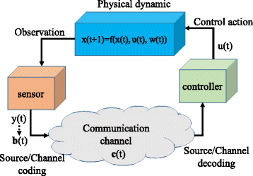

  

  An illustration of the components in CPSs

• How much gain can be obtained by using redundancy of observations in time domain to assist channel decoding?

As pointed out before, the CPS is a hybrid system [2], which consists of system state x(t), observation y(t) with continuous values, and information bits b(t) transmitted in wireless communication with discrete values. The challenges in the channel decoding and system state estimation framework are that the priori information transmitted from a state estimator to a channel decoder is the prediction of y(t), while the channel decoder actually requires the priori information of each quantized bit of y(t), and that the output of the channel decoder is the extrinsic information of each quantized bit of y(t), while the state estimator actually requires the estimation of y(t) from the channel decoder. To handle these challenges, two models, the BP-based sequential model and the BP-based iterative model, are given to evaluate the performance of BP-based channel decoding and system state estimation framework. The former can be used to evaluate the performance of system state estimation over multiple time slots, e.g., the gain by utilizing priori information from the previous time slot to assist channel decoding and state estimation at the current time slot. The latter can be used to check the following points:

• 1. Does the iterative channel decoding and estimation converge, and how many iterations are sufficient?

• 2. How much gain can be obtained by utilizing priori information from the previous time slots to assist state estimation at the current time slot?

In the area of wireless communication, the purpose of performance analysis for decoding scheme is to find out if, for any given encoder, decoder, and channel noise power, a message-passing iterative decoder can correct the errors or not.

To analyze the performance, in [3–5], Ten Brink proposed using an extrinsic information transfer (EXIT) chart to track the iterative decoding performance. Based on the assumption that the distribution of the extrinsic log-likelihood ratios (LLRs) is a Gaussian distribution, the EXIT chart tracks mutual information from the extrinsic LLRs through an iterative decoding process. Compared with the previously used method of density evolution, the EXIT chart is computationally simplified, and it also allows to visualize the evolution of mutual information through iterative decoding process in a graph. The details of the EXIT chart can be found in [6].

The EXIT chart has two useful properties as shown in [7]. One is the necessary condition for the convergence of iterative decoding that the flipped EXIT chart curve of the outer decoder for iterations lies below the EXIT chart curve of the inner coder. The other is that the area under the EXIT curve of outer code relates to the rate of inner coder. In [8], the authors demonstrated that if the priori channel is an erasure channel, for any outer code of rate R, the area under the EXIT curve is 1−R. To our best knowledge, the area property of the EXIT chart has been proved only for cases where the priori channels are erasure channels.

The mean square error (MSE) transfer chart improves the EXIT chart as shown in [7], because the area property of the MSE transfer chart corresponding to the area property of the EXIT charts has been proven in both erasure channels and AWGN channels. Instead of tracking mutual information, the MSE transfer chart, as an alternative to evaluate decoding performance, has been proposed in [9] to track the iterative decoding performance based on the relationship between mutual information and the minimum mean square error (MMSE) for the additive white Gaussian noise (AWGN) channel.

In this paper, we use the MSE transfer chart to analyze the message passing procedure of channel decoding and system state estimation by assuming that the priori information is an AWGN channel. Compared with [9], our hybrid model prioritizes practicality because the system states and observations considered are continuous values while the information transmitted in wireless system are quantized information bits. Unlike previous research, our algorithm addresses the message passing between continuous values from the state estimator and quantized information bits from the channel decoder with the condition that the system state is correlated over different time slots. In addition, in order to view the evolution of the estimation error, we analyze the performance of state estimation in two cases: within two time slots and more than two time slots.

Our work is also informed by other areas in wireless communication, which have faced similar issues in source coding (quantization) [10–13] and joint source and channel decoding [14–19]. The idea of source coding (quantization) in the context of this work is combining the side information available at the controller to assist system state estimation, and the route of joint source and channel decoding in [20–25] is to utilize redundancy in the source to assist channel decoding. Our work can also be considered as one special case of joint source and channel decoding. However, there are two major differences. One difference is that most works focus on the source with binary values and use the EXIT chart [26, 27] or the protograph EXIT (PEXIT) [16] for performance analysis, while [28, 29] considered the case with the source of non-binary values, but the performance analysis of decoding was not provided. The other difference is that most works, such as [29], considered the joint source and channel decoding within two time slots. For instance, only the estimation from the previous time slot is used to calculate the estimation of current time slot. In our work, the dynamic state changes over more than two time slots, and the performance of channel decoding and system estimation at the current time slots also impacts its performance in all future time slots. Therefore, we study the performance of iterative estimation and decoding across multiple time slots.

This paper is organized as following. Following the review of the literature on iterative decoding performance analysis method in Section 1, Section 2 briefly introduces on the EXIT chart and the MSE transfer chart for the performance evaluation of iterative channel decoding. Section 3 describes the system models for performance analysis. Section 4 presents the message passing framework between system observation and channel decoding. Section 5 describes the MSE transfer chart, and Section 6 presents how to use the MSE transfer chart to evaluate BP-based sequential and iterative channel decoding and state estimation. Finally, a brief conclusion is given in Section 7.

2 Preliminaries on the EXIT Chart

In this section, we review the concept of the EXIT chart and the MSE transfer chart by iterative decoding the output of a serially concatenated encoder. In Section 2.1, we use an example to illustrate the serially concatenated coding scheme and its iterative decoding process. Then, in Section 2.2, we review how to use the EXIT chart and the MSE transfer chart to analyze the performance of iterative decoding.

2.1 A serially concatenated encoding scheme and corresponding iterative decoding algorithm

Figure 2 shows a simple serially concatenated encoding scheme and its corresponding iterative decoding scheme.

Fig. 2

A demo of concatenated encoding and iterative decoding

At the transmitter, the source S with binary values is a vector with the length L _s , i.e., $\phantom {\dot {i}\!}\mathbf {S}=[S_{1}, \cdot \cdot \cdot, S_{L_{s}}]$. S is encoded by the outer channel encoder, which is a systematic convolutional encoder whose generator is g _out with an output of B _out, a vector with the length L _out. Next, B _out is encoded by the inner channel encoder, also a systematic convolutional encoder whose the generator is g _in with an output of B _in, a vector with the length L _in. Finally, B _in is modulated with an output of B _m , i.e., B _m,i =2B _in,i −1, i=1,···,L _in, and then sent over an AWGN channel with an output that can be calculated by

$$ Y_{\text{in}, i}=B_{m,i} +\frac{1}{\sqrt{\text{SNR}}}v_{i}\quad i=1,\cdot\cdot\cdot, L_{\text{in}} $$

(1)

where $\text {SNR}=\frac {E_{b}}{N_{0}}$ is the signal power to noise power ratio and v _i is a zero mean and unit variance Gaussian noise.

At the receiver, decoding is done iteratively between the inner decoder and the outer decoder. The inputs for the inner channel decoder are the received signal Y _in and a priori information from the outer decoder, i.e., $\mathbf {L}_{A}^{\text {in}, k}=\mathbf {L}_{E}^{\text {out}, k-1}$, where $\mathbf {L}_{E}^{\text {out}, k-1}$ is the extrinsic information of the outer decoder from (k−1)th decoding round, and the output for it is $\mathbf {L}_{E}^{\text {in}, k}$, i.e.,

$$ \mathbf{L}_{E, i}^{\text{in}, k}= \text{LLR}\left(S_{i} |\mathbf{Y}_{\text{in}}, \mathbf{L}_{A,i}^{\text{in}, k}, g_{\text{in}}\right) \quad i=1,\cdot\cdot\cdot, L_{s} $$

(2)

where $\mathbf {L}_{A,i}^{\text {in}, k}$ means the priori information of $\mathbf {L}_{A,i}^{\text {in}, k}$ for all S except S _i . The input for the outer channel decoder is a priori information from the inner decoder, i.e., $\mathbf {L}_{A}^{\text {out}, k}=\mathbf {L}_{E}^{\text {in}, k}$, and the output for it is $\mathbf {L}_{E}^{\text {out}, k}$, i.e.,

$$ \mathbf{L}_{E,i}^{\text{out}, k}= \text{LLR}\left(S_{i} |\mathbf{L}_{A,i}^{\text{out}, k}, g_{\text{out}}\right) \quad i=1,\cdot\cdot\cdot, L_{s} $$

(3)

where $\mathbf {L}_{A,i}^{\text {out}, k}$ means the priori information of $\mathbf {L}_{A,i}^{\text {out}, k}$ for all S except S _i .

2.2 The EXIT chart and the MSE transfer chart

The iterative decoding scheme in [30] can be analyzed by tracking the density evolution over iterations. However, the density evolution is complex as it requires to obtain probability density function (PDF) of extrinsic LLRs for each iteration; in addition, it does not provide much insight about the operations of iterative decoding. In order to overcome the drawbacks of density evolution, many transfer chart-based analysis frameworks have been proposed, such as the EXIT chart by [3–5] and the MSE transfer chart by [9]. The idea of these transfer chart-based analysis frameworks is to approximate the PDF of extrinsic LLRs exchanged between the inner decoder and outer decoder by a parameter, i.e.,

$$ F(\mathbf{S, L})=\frac{1}{L_{s}} {\sum\nolimits}_{i=1}^{L_{s}}F(S_{i}, \mathbf{L}_{i}),\quad i=1, \cdot\cdot\cdot, L_{s} $$

(4)

where L _i is the extrinsic information, i.e. $\mathbf {L}_{E,i}^{\text {out}, k}, \mathbf {L}_{E,i}^{\text {in}, k}, \mathbf {L}_{A,i}^{\text {out}, k}$, and $\mathbf {L}_{A,i}^{\text {in}, k}$.

The measure used by the EXIT chart is mutual information, i.e., F(S , L)=I(S , L), which is based on the observation that the PDF of extrinsic LLRs can be approximated by a Gaussian distribution [3–5].

The measure used by the MSE transfer chart is F(S , L)=E[ tanh2(L/2)], which is related to the MMSE estimation of S based on observation Y _in [9], i.e.,

$$ \left\{\begin{array}{rl}\!\! \text{MMSE}\left(\mathbf{S}| \mathbf{Y}_{\text{in}}\right)\!&=\!E\left[\left(\mathbf{S}\,-\,\hat{\mathbf{S}}\right)^{2}|\mathbf{Y}_{\text{in}}\! \right]\!=1-E\left[\tanh^{2}\left(\mathbf{L}/2\right)\right]\\ \hat{\mathbf{S}}&=E\left[{\mathbf{S}}|\mathbf{Y}_{\text{in}} \right]= \tanh(\mathbf{L}/2)\\ \mathbf{L}&=\text{LLR}\left({\mathbf{S}}|\mathbf{Y}_{\text{in}}\right)=\log \left(\frac{P\left(\mathbf{S}=1, \mathbf{Y}_{\text{in}} \right)}{P\left(\mathbf{S}=-1, \mathbf{Y}_{\text{in}} \right)}\right) \end{array}\right. $$

(5)

The EXIT chart and the MSE transfer chart-based decoding frameworks for a serially concatenated encoding scheme are shown in Fig. 3 (a and b), respectively. The transfer chart includes two transfer curves. One curve is the measure for the priori information of inner decoder, i.e., $F_{A}^{\text {in}}(\mathbf {S, L})$, versus the measure for the extrinsic information of inner decoder, i.e., $F_{E}^{\text {in}}(\mathbf {S, L})$; the other curve is the measure for the priori information of outer decoder, i.e., $F_{A}^{\text {out}}(\mathbf {S, L})$, versus the measure for the extrinsic information of outer decoder, i.e., $F_{E}^{\text {out}}(\mathbf {S, L})$. The EXIT chart and the MSE transfer chart for the serially concatenated coding scheme are shown in Figs. 4 and 5, respectively. The predicted decoding path is also shown in these two figures. Since there is a decoding path found between the two curves, the iterative decoding converges.

Fig. 3

The EXIT chart and the MSE transfer chart model for concatenated encoding and iterative decoding. a EXIT chart. b MSE based transfer chart

Fig. 4

An example of the EXIT chart for concatenated encoding and iterative decoding, g _out=g _in=[1,1,0,1;1,0,0,1],SNR=−2 dB

Fig. 5

An example of the MSE transfer chart for concatenated encoding and iterative decoding, g _out=g _in=[1,1,0,1;1,0,0,1],SNR=−2 dB

3 System model

In this section, we describe the system model for the analysis.

3.1 Linear dynamic system and communication system

We consider a discrete time linear dynamic system, whose state evolution is given by

$$ \left\{\begin{array}{lll} \mathbf{x}(t+1)&=&\mathbf{A}\mathbf{x}(t)+\mathbf{B} \mathbf{u}(t)+ \mathbf{n}(t)\\ \mathbf{y}(t)&=&\mathbf{C}\mathbf{x}(t)+ \mathbf{w}(t) \end{array}\right. $$

(6)

where x(t) is the N-dimensional vector of system state at time slot t, u(t) is the M-dimensional control vector, y(t) is the K-dimensional observation vector, and n(t) and w(t) are noise vectors, which are assumed to be Gaussian distributions with zero mean and covariance matrix Σ _n and Σ _w , respectively. For simplicity, we do not consider u(t).

Additionally, we assume that the observation vector y(t) is obtained by a sensor¹, and the sensor quantizes each dimension of the observation vector y(t) using B bits, thus forming a KB-dimensional binary vector, which is given by

$$ \mathbf{b}(t)=\left(b_{1}(t), b_{2}(t), \ldots, b_{KB}(t)\right) $$

(7)

The information bits b(t) are then put into an encoder to generate a codeword c(t). Suppose that the binary phase-shift keying (BPSK) is used for the transmission between the sensor and the controller, and c(t) is converted to alphabet {−1,+1} with s(t)=2c(t)−1. Next, the sequence s(t) is passed through a modulator and transmitted into an AWGN channel. Then, the received signal at the controller is given by

$$ \mathbf{r}(t)=\mathbf{s}(t)+\mathbf{e}(t) $$

(8)

where the additive white Gaussian noise e(t) has a zero expectation and variance Σ _c . Note that we consider the AWGN channel, ignore the fading and normalize the transmit power to be 1. The algorithm and conclusion in this work can be easily extended to the cases with different channels and different types of fading.

3.2 Models for belief propagation based channel decoding and state estimation

In this section, we firstly introduce the Bayesian network structure and then use the following two models to evaluate BP-based channel decoding and state estimation: BP-based sequential processing and BP-based iterative processing.

3.2.1 Bayesian network structure and the message passing

The Bayesian network structure of the dynamic system and communication system is shown in Fig. 6, where the message passing in the system is illustrated by dotted arrows and dashed arrows in the figure with three time slots: x(t−2),x(t−1), and x(t). The dashed arrows transmit π-message from a parent to its children in Pearl’s BP, and the details and formal description can be found in [31]. For instance, the message passed from x(t−2) to x(t−1) is π _{x(t−2),x(t−1)}(x(t−2)), which is the priori information of x(t−2) given that all the information x(t−2) has been received. The dotted arrows transmit λ-message from a child to its parent. For instance, the message passed from x(t−1) to x(t−2) is λ _{x(t−1),x(t−2)}(x(t−2)), which is the likelihood of x(t−2) given that the information x(t−1) has been received.

Fig. 6

Bayesian network structure and the message passing for CPSs

Note that the π-message and λ-message are passing in the form of probability distribution function (PDF), and based on the Bayesian network structure in Fig. 6 and Pearl’s BP, the updating order and the message passing in one iteration is given as follows: step 1: x(t−1)→y(t−1); step 2: y(t−1)→b(t−1); step 3: b(t−1)→y(t−1); step 4: y(t−1)→x(t−1); step 5: x(t−1)→x(t); step 6: x(t)→y(t); step 7: y(t)→b(t); step 8: b(t)→y(t); step 9: y(t)→x(t); step 10: x(t)→x(t−1); and step 11: x(t−1) updates information. The key steps in the Pearl’s BP have be derived as shown in Table 1, where the PDF of λ _b(t),y(t)(y(t)) will be computed by iterative decoding provided in Section 4.

Table 1 Message passing in BP-based channel decoding and state estimation system

3.2.2 Model for BP-based sequential processing

Based on the Bayesian network structure in Fig. 6, we use the framework as shown in Fig. 7 (a) to evaluate sequential channel decoding and state estimation over more than two time slots. The priori information from the time slot t−1, i.e., π _{x(t−1),x(t)}(x(t−1)), is used to assist channel decoding and state estimation at the time slot t, i.e., the estimated distribution of x(t−1), and we assume that it is also a Gaussian distribution with mean $\mathbf {x}_{\pi _{x},t-1}$ and covariance matrix $\mathbf {P}_{\pi _{x},t-1}$, i.e., $\mathcal {N}(\mathbf {x}_{t-1}, \mathbf {x}_{\pi _{x},t-1}, \mathbf {P}_{\pi _{x},t-1})$.

Fig. 7

a Sequential channel decoding and state estimation, b The measure of sequential channel decoding and state estimation

As noted in Section 1, two objectives here are to evaluate how much gain can be obtained by utilizing π _{x(t−1),x(t)}(x(t−1)) to assist channel decoding and state estimation at time slot t and to evaluate the performance of state estimation over multiple time slots, i.e., the evolution of $\mathbf {P}_{\pi _{x},t-1}$ as shown in Fig. 7(b).

3.2.3 Model for BP-based iterative processing between two time slots

Figure 8(a) illustrates the model used to evaluate BP-based iterative channel decoding and state estimation between two time slots. The inputs for this model include the received signals at the controller within the two time slots, i.e., r(t) and r(t+1), which can be found in Fig. 6, and the priori information from the previous time slot t−1, i.e., π _{x(t−1),x(t)}(x(t−1)).

Fig. 8

Model for the iterative message passing with priori information from x(t−1). a Iterative channel decoding and state estimation, b Iterative channel decoding and state estimation with previous observation, c Iterative channel decoding and state estimation without previous observation

The goal is to evaluate the performance of iterative channel decoding and state estimation for different realizations of the two distributions for π _{x(t−1),x(t)}(x(t−1)). For instance, when π _{x(t−1),x(t)}(x(t−1)) (say, $\mathbf {P}_{\pi _{x},t-1}$) equals to 0×I, x(t−1) is a determined state estimation. Therefore, this reference model can be converted to the model shown in Fig. 8 (b) by setting π _{x(t−1),x(t)}(x(t−1) (say, $\mathbf {P}_{\pi _{x},t-1}$) as 0×I. Or if π _{x(t−1),x(t)}(x(t−1)) (say, $\mathbf {P}_{\pi _{x},t-1}$) is set as ∞×I, x(t−1) is unknown. Then, the reference model is transformed to the model shown in Fig. 8 (c).

4 Message passing between state estimator and channel decoder

In this section, we describe the message passing between state estimator and channel decoder, which is the most challenging and vital part for the evaluation of BP-based channel decoding and state estimation. As stated in Table 1, π _y(t),b(t)(y(t)) has been assumed to be a Gaussian distribution with the mean y _π,t and the covariance matrix S _π,t and λ _b(t),y(t)(y(t)) with the mean y _λ,t and covariance matrix S _λ,t . We can simplify the procedure of the message exchanging by substituting π _y(t),b(t)(y(t)) and λ _b(t),y(t)(y(t)) with S _π,t and S _λ,t , respectively, as shown in Fig. 9. Below, we explain how the averaging S _λ,t , i.e., $\bar {\mathbf {S}}_{\lambda, t}$, corresponding to S _π,t can be computed by using iterative decoding.

Fig. 9

Information exchange between channel decoder and state estimator

Quantizing the message between channel decoder and state estimator

The relationships among y _π,t , S _π,t , y ^′(t), and channel noise are shown in Fig. 10, where y ^′(t) is one realization of π _y(t),b(t)(y(t)). Then, y ^′(t) is quantized, modulated, and transmitted over the wireless channel. We denote the corresponding quantized vector, modulated vector, channel noise vector, and received vector as b ^′(t), c ^′(t), e ^′(t) and r ^′(t), respectively.

Fig. 10

Model for S _λ,t based on sample y _π,t , S _π,t , y ^′(t), and e ^′(t)

The physical meaning of π _y(t),b(t)(y(t)) is the PDF of y(t). Next, we can use π _y(t),b(t)(y(t)) as the priori information to estimate each bit of b(t) based on its quantization scheme (the quantization scheme used for converting y(t) to b(t)), i.e., L _A (y _π,t ,S _π,t ). Note that L _A (y _π,t ,S _π,t ) is determined by the PDF, i.e., π _y(t),b(t)(y(t)), and also the quantization scheme. Thus, L _A (y _π,t ,S _π,t ) is a KB-dimensional vector and its ith element can be calculated as

$$ {} \mathbf{L}_{A,i}\left(\mathbf{y}_{\pi, t}, \mathbf{S}_{\pi, t}\right) =\log \frac{P\left(b_{i}(t)=1|\mathbf{y}(t) \in \mathcal{N}\left(\mathbf{y}_{t}, \mathbf{y}_{\pi, t}, \mathbf{S}_{\pi, t}\right)\right)}{P\left(b_{i}(t)=0|\mathbf{y}(t) \in \mathcal{N}\left(\mathbf{y}_{t}, \mathbf{y}_{\pi, t}, \mathbf{S}_{\pi, t}\right)\right)} $$

(9)

The inputs for the channel decoder are L _A (y _π,t ,S _π,t ) and r ^′(t) shown in Fig. 10. The feedback from the channel decoder to the state estimator is the extrinsic LLR, which is denoted as L _E (L _A (y _π,t ,S _π,t ),y ^′(t),e ^′(t)). It is a KB-dimension vector and its ith element equals to

$$ \begin{aligned} &\mathbf{L}_{E, i}\left(\mathbf{L}_{A}\left(\mathbf{y}_{\pi, t}, \mathbf{S}_{\pi, t}\right), \mathbf{y}^{\prime}(t), \mathbf{e}^{\prime}(t)\right)\\ &\qquad\qquad=\log \frac{P\left(b_{i}(t)=1|\mathbf{L}_{A}\left(\mathbf{y}_{\pi, t}, \mathbf{S}_{\pi, t}\right), \mathbf{r}^{\prime}(t)\right)}{P\left(b_{i}(t)=0|\mathbf{L}_{A}\left(\mathbf{y}_{\pi, t}, \mathbf{S}_{\pi, t}\right), \mathbf{r}^{\prime}(t)\right)} \end{aligned} $$

(10)

Note that L _E (L _A (y _π,t ,S _π,t ),y ^′(t),e ^′(t)) depends on L _A (y _π,t ,S _π,t ), y ^′(t), and e ^′(t). Based on L _E (L _A (y _π,t ,S _π,t ),y ^′(t),e ^′(t)), if we assume c(t)=b(t), based on [7], b _i (t) can be estimated as

$$ \begin{aligned} \tilde{\mathbf{b}}_{i}(t)&=\frac{1}{2}\left(\tilde{\mathbf{s}}_{i}(t)+1\right)\\ &=\frac{1}{2}\tanh\left\{\frac{L_{E,i}\left[\mathbf{L}_{A}\left(\mathbf{y}_{\pi, t},\mathbf{S}_{\pi, t} \right), \mathbf{y}^{\prime}(t), \mathbf{e}^{\prime}(t)\right]}{2}\right\} +\frac{1}{2} \end{aligned} $$

(11)

where $\tilde {\mathbf {s}}_{i}(t)$ is the estimated-modulated bit and the MMSE in estimating b _i (t) from L _E (L _A (y _π,t ,S _π,t ),y ^′(t),e ^′(t)) is given as

$$ \begin{aligned} &\text{MMSE}_{\mathbf{b}_{i}(t)}\\ &\quad=\text{MMSE}\left({\mathbf{b}}_{i}(t)|\mathbf{L}_{E}\left(\mathbf{L}_{A}\left(\mathbf{y}_{\pi, t}, \mathbf{S}_{\pi, t}\right), \mathbf{y}^{\prime}(t), \mathbf{e}^{\prime}(t)\right)\right)\\ &\quad=\frac{1}{4} -\frac{1}{4}\tanh^{2}\left(\frac{L_{E,i}\left[\mathbf{L}_{A}\left(\mathbf{y}_{\pi, t},\mathbf{S}_{\pi, t} \right), \mathbf{y}^{\prime}(t), \mathbf{e}^{\prime}(t)\right] }{2}\right) \end{aligned} $$

(12)

Then, y(t) can be estimated as

$$\begin{array}{*{20}l} \tilde{\mathbf{y}}_{k}(t)=Q_{I} \sum_{i=1}^{B} \tilde{\mathbf{b}}_{(k-1)B+i}(t) 2^{i-1}+Q_{\text{min}} \end{array} $$

(13)

and the MMSE in estimating y _k (t) is given by

$$ \begin{aligned} &\text{MMSE}_{\mathbf{y}_{k}(t)}\\ &\quad=\text{MMSE}\left({\mathbf{y}}_{k}(t)|\mathbf{L}_{E}\left(\mathbf{L}_{A}\left(\mathbf{y}_{\pi, t}, \mathbf{S}_{\pi, t}\right), \mathbf{y}^{\prime}(t), \mathbf{e}^{\prime}(t)\right)\right)\\ &\quad= (Q_{I})^{2} E\left\{\sum_{i=1}^{B}[ \tilde{\mathbf{b}}_{(k-1)B+i}(t) - {\mathbf{b}}_{(k-1)B+i}(t)]2^{i-1}\right\}^{2}\\ &\quad= (Q_{I})^{2} \sum_{i=1}^{B}\text{MMSE}_{\mathbf{b}_{i}(t)} 2^{2(i-1)} \end{aligned} $$

(14)

where [Q _min,Q _max] is the range for quantization and Q _I is the quantization interval, which is given as $Q_{I}=\frac {Q_{\text {max}}-Q_{\text {min}}}{2^{B}-1}$. Note that when i≠j, $E\{[ \tilde {\mathbf {b}}_{(k-1)B+i}(t) - {\mathbf {b}}_{(k-1)B+i}(t)][ \tilde {\mathbf {b}}_{(k-1)B+j}(t) - {\mathbf {b}}_{(k-1)B+j}(t)]\}=0$, which is obtained based on the independence of channel noise and required for the derivation of (14).

Then, for a given π _y(t),b(t)(y(t)), which has PDF as $\mathcal {N}(\mathbf {y}_{t}, \mathbf {y}_{\pi, t}, \mathbf {S}_{\pi, t})$, a realization y ^′(t), and a channel noise e ^′(t), the feedback from the channel decoder to the node y(t) is λ _b(t),y(t)(y(t)), corresponding to $\mathcal {N}(\mathbf {y}_{t}, \mathbf {y}_{\lambda, t}, \mathbf {S}_{\lambda, t})$, whose mean and covariance matrix are given as

$$ \begin{aligned} \mathbf{y}_{\lambda, t}&=\left[\tilde{\mathbf{y}}_{1}(t), \cdot\cdot\cdot,\tilde{\mathbf{y}}_{K}(t)\right]\\ \mathbf{S}_{\lambda, t}(k,k)&=\text{MMSE}_{\mathbf{y}_{k}(t)} \end{aligned} $$

(15)

Thus, we finalize the computation of $\mathcal {N}(\mathbf {y}_{t}, \mathbf {y}_{\lambda, t}, \mathbf {S}_{\lambda, t})$ based on one realization, y ^′(t), which is obtained from the PDF of π _y(t),b(t)(y(t)).

Approximation for the message passing between state estimator and channel decoder

As shown in Fig. 11 (a), for a given π _y(t),b(t)(y(t)), the extrinsic information transferred from the channel decoder to the node y(t) can be computed as

$$ \begin{aligned} &\mathbf{S}_{\lambda, t}\left(\mathbf{y}_{\pi, t}, \mathbf{S}_{\pi, t}\right) \\ &= {E}_{\mathbf{y}^{\prime}(t)\in\pi_{\mathbf{y}(t), \mathbf{b}(t)}(\mathbf{y}(t)), \mathbf{e}^{\prime}(t) }\left[\text{MMSE}_{\mathbf{y}_{k}(t)}\right] \end{aligned} $$

(16)

Fig. 11

Framework for S _λ,t averaging over y ^′(t) and e ^′(t)

And, as shown in Fig. 11 (b), if we denote the PDF of y _π,t as $\phantom {\dot {i}\!}f_{\mathbf {y}_{\pi, t}}$, we can obtain the average S _λ,t corresponding to S _π,t by integrating S _λ,t (y _π,t ,S _π,t ) over y _π,t ,

$$ \begin{aligned} \mathbf{S}_{\lambda, t}(\mathbf{S}_{\pi, t}) &={E}_{\mathbf{y}_{\pi, t}}\left[\mathbf{S}_{\lambda, t}\left(\mathbf{y}_{\pi, t}, \mathbf{S}_{\pi, t}\right)\right]\\ &= {E}_{\mathbf{y}_{\pi, t}}\left\{{E}_{\mathbf{y}^{\prime}(t)\in\pi_{\mathbf{y}(t), \mathbf{b}(t)}(\mathbf{y}(t)), \mathbf{e}^{\prime}(t)}\left[\text{MMSE}_{\mathbf{y}_{k}(t)}\right]\right\} \end{aligned} $$

(17)

Note that the computation of S _λ,t (S _π,t ) in (17) would require the averaging over a sufficient number of realizations (i.e., large enough to show the probability distribution based on a fixed y _π,t ) of y ^′(t) and the averaging over all possible y _π,t based on its PDF $\phantom {\dot {i}\!}f_{\mathbf {y}_{\pi, t}}$ to be computed sequentially, i.e., Forward Process and Backward Process should be calculated sequentially. The Forward Process generally refers to the message passing from a node to its children, and the Backward Process generally refers to the message passing from a node to its parents. This arises because y _π,t not only impacts priori information L _A (y _π,t ,S _π,t ) but also defines the set of codewords which are generated by quantizing y ^′(t).

However, the computation as discussed above prohibits the independent evaluation of the message passing for Forward Process and Backward Process. Thus, to bypass this difficulty, we make the following approximations for the computation of S _λ,t (S _π,t ), so that the Forward Process and Backward Process can be considered separately:

$$ \begin{aligned} \mathbf{S}_{\lambda, t}(\mathbf{S}_{\pi, t}) &={E}_{\mathbf{y}_{\pi, t}}\left[\mathbf{S}_{\lambda, t}\left(\mathbf{y}_{\pi, t}, \mathbf{S}_{\pi, t}\right)\right]\\ &= {E}_{\mathbf{y}_{\pi, t}}\left\{{E}_{\mathbf{y}^{\prime}(t)\in\boldsymbol{U}(\mathbf{R}(\mathbf{y})), \mathbf{e}^{\prime}(t) }\left[\text{MMSE}_{\mathbf{y}_{k}(t)}\right]\right\}\\ &= {E}_{\mathbf{y}_{\pi, t}, \mathbf{y}^{\prime}(t)\in\boldsymbol{U}(\mathbf{R}(\mathbf{y})), \mathbf{e}^{\prime}(t) }\left[\text{MMSE}_{\mathbf{y}_{k}(t)}\right]\\ &= {E}_{\mathbf{L}_{A}\left(\mathbf{y}_{\pi, t},\mathbf{S}_{\pi, t}\right), \mathbf{y}^{\prime}(t)\in\boldsymbol{U}(\mathbf{R}(\mathbf{y})), \mathbf{e}^{\prime}(t) }\left[\text{MMSE}_{\mathbf{y}_{k}(t)}\right] \end{aligned} $$

(18)

First, we approximate the PDF of the realizations y ^′(t) as a uniform distribution instead of $\mathcal {N}(\mathbf {y}_{t}, \mathbf {y}_{\pi, t}, \mathbf {S}_{\pi, t})$, and we denote the uniform distribution as U(R(y)), where R(y) is the range of y(t). Given this approximation, the integration of y ^′(t) over U(R(y)) is equivalent to the integration of all codewords with an equal probability, and hence, the realization y ^′(t) can be viewed as being independent of π _y(t),b(t)(y(t)). Next, as shown in the final step of (18), the averaging over y _π,t can be changed to the averaging over L _A (y _π,t ,S _π,t ). This exists because y _π,t impacts only priori information L _A (y _π,t ,S _π,t ) and the set L _A (y _π,t ,S _π,t ) includes all information from y _π,t . The framework equivalent to (18) is shown in Fig. 12 (a), which is denoted as approximate framework 1, and the computation of S _λ,t (S _π,t ) in (18) can be divided into the following three steps:

• 1. Compute the PDF of L _A (y _π,t ,S _π,t ) and $\phantom {\dot {i}\!}f_{\mathbf {y}_{\pi,t}}$.

  Fig. 12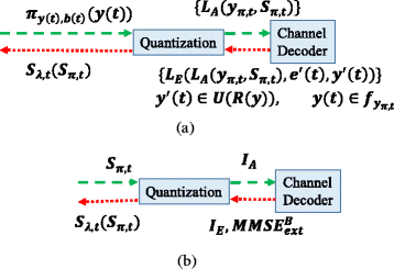

  

  Approximate framework for S _λ,t averaging over y ^′(t), e ^′(t) and y _π,t . a Approximate Framework 1. b Approximate Framework 2

• 2. Compute the extrinsic information from the channel decoder, i.e., the PDF of L _E (L _A (y _π,t ,S _π,t ),y ^′(t),e ^′(t)).

• 3. Compute S _λ,t (S _π,t ) from the extrinsic information L _E (L _A (y _π,t ,S _π,t ),y ^′(t),e ^′(t)).

Second, we can approximate the PDF of both L _A (y _π,t ,S _π,t ) and L _E (L _A (y _π,t ,S _π,t ), y ^′(t), e ^′(t)) as the Gaussian distributions with zero means. Next, only the covariance matrixes need to be passed through the decoding process. Note that L _E (L _A (y _π,t ,S _π,t ),y ^′(t),e ^′(t)) for different bits might have a huge difference. This Gaussian approximation requires a good interleaver which can evenly distribute L _E (L _A (y _π,t ,S _π,t ),y ^′(t),e ^′(t)). Furthermore, if we represent the LLRs by mutual information or MMSE [7] as shown in Fig. 12(b), S _λ,t (S _π,t ) can be computed in the following three steps:

• 1. Compute the mutual information I _A based on the PDF of L _A (y _π,t ,S _π,t ) corresponding to S _π,t and $\phantom {\dot {i}\!}f_{\mathbf {y}_{\pi,t}}$.

• 2. Compute the extrinsic information from the channel decoder, i.e., mutual information I _E or $\text {MMSE}_{\text {ext}}^{B}$ based on the PDF of L _E (L _A (y _π,t ,S _π,t ),y ^′(t)),e ^′(t)).

• 3. Compute S _λ,t (S _π,t ) from the extrinsic information of the channel decoder I _E or $\text {MMSE}_{\text {ext}}^{B}$.

5 The MSE transfer chart for channel decoding and state estimation

In this section, we show how to obtain the MSE transfer chart for evaluating BP-based sequential channel decoding and state estimation as shown in Fig. 7(b) and BP-based iterative channel decoding and state estimation as shown in Fig. 8(a).

5.1 The MSE transfer chart for sequential channel decoding and state estimation

The corresponding model to Fig. 7(b) for the MSE transfer chart of the sequential message passing is illustrated in Fig. 13 (a). The MSE transfer chart for BP-based sequential channel decoding and state estimation shows the curves between $\text {MMSE}_{\text {ap}}^{S}$ versus $\text {MMSE}_{\text {ext}}^{S}$. As shown in Fig. 13 (a), $\text {MMSE}_{\text {ap}}^{S}$ is used to approximate S _π,t (starting from node y(t)), i.e.,

$$ \mathbf{S}_{\pi, t}=\text{MMSE}_{\text{ap}}^{S}\mathbf{I}_{K} $$

(19)

Fig. 13

The MSE transfer chart for the sequential message passing and iterative message passing. a Sequential message passing. b Iterative message passing

and the PDF y _π,t , i.e., $\phantom {\dot {i}\!}f_{\mathbf {y}_{\pi, t}}$, is assumed to keep the same in all time slots and all iterations. Similarly, $\text {MMSE}_{\text {ext}}^{S}$ represents the averaging S _π,t+1 corresponding to S _π,t and y _π,t with the PDF of $\phantom {\dot {i}\!}f_{\mathbf {y}_{\pi, t}}$.

Compared with the model shown in Fig. 7 (b), the MSE transfer chart has two differences. First, the starting node for the message passing is changed from x(t−1) to y(t). The reason for this changing is to keep alignment with the structure of the MSE transfer chart for BP-based iterative channel decoding and state estimation. Note that since there is no extra information added from node x(t−1) to y(t), x(t−1) and y(t) provide the same amount of information for channel decoding in the context of information theory. From this point, these two models are equivalent. The second modification is that the scalar measures, to draw the MSE transfer chart $\text {MMSE}_{\text {ap}}^{S}$ and $\text {MMSE}_{\text {ext}}^{S}$, rather than the matrix measures are used to evaluate the performance of the sequential message passing.

The value of $\text {MMSE}_{\text {ext}}^{S}$ can be obtained by applying the results in Table 1, and the message passing flow is shown as

• 1. y(t)→b(t), we have $\mathbf {S}_{\pi, t}=\text {MMSE}_{\text {ap}}^{S}\mathbf {I}_{K}$ and the PDF of y _π,t is $\phantom {\dot {i}\!}f_{\mathbf {y}_{\pi, t}}$.

• 2. b(t)→y(t), S _λ,t , the detailed derivation is provided in Section 4.

• 3. y(t)→x(t), we have $\mathbf {P}_{\lambda _{y},t} = \mathbf {C}^{-1} (\mathbf {S}_{\lambda, t}+\mathbf {\Sigma }_{w})(\mathbf {C}^{-1})^{T}$.

• 4. x(t)→x(t+1), we have $\mathbf {P}_{\pi _{x},t}=(\mathbf {P}_{l,t}^{-1}+\mathbf {P}_{\lambda _{y},t}^{-1})^{-1}$, where $\mathbf {P}_{l, t} = \mathbf {A} \mathbf {P}_{\pi _{x},t-1} \mathbf {A}^{T} +\mathbf {\Sigma }_{n}$.

• 5. x(t+1)→y(t+1), we have $\mathbf {P}_{\pi _{y},t+1}=\mathbf {A}\times \mathbf {P}_{\pi _{x},t+1}\times \mathbf {A}^{T} +\mathbf {\Sigma }_{n}$.

• 6. y(t+1)→b(t+1), we have $\mathbf {S}_{\pi,t+1}=\mathbf {C}\times \mathbf {P}_{\pi _{y},t+1}\times \mathbf {C}^{T} +\mathbf {\Sigma }_{w}$. Note that S _π,t+1 is a matrix, $\text {MMSE}_{\text {ext}}^{S}$ is calculated by solving the following equation:

  $$ I_{A}(\text{MMSE}_{\text{ext}}^{S}\mathbf{I}_{K})=I_{A}(\mathbf{S}_{\pi,t+1}) $$

  (20)

where we first obtain the priori information I _A for each ith diagonal variance of S _π,t+1, where i∈{1,..,K}. Next, to achieve (20), we compute the average value of all the variances, as $\text {MMSE}_{\text {ext}}^{S}$. An example of the calculation will be illustrated Section 6.1 in Fig. 15. The physical meaning of (20) is that $\text {MMSE}_{\text {ext}}^{S}$ is the value such that $\text {MMSE}_{\text {ext}}^{S}\mathbf {I}_{K}$ can provide the same amount of priori information for the channel decoder as S _π,t+1.

5.2 The MSE transfer chart for BP-based iterative channel decoding and state estimation

In this section, we illustrate how the MSE transfer chart is modeled in order to evaluate the BP-based iterative channel decoding and state estimation as shown in Fig. 8 (a). The corresponding model for the MSE transfer chart is shown in Fig. 13(b), and it includes two flows of the message passing: one from y(t) to y(t+1) in Fig. 14(a) and the other from y(t+1) to y(t) in Fig. 14(b).

• 1. The flow from y(t) to y(t+1): the starting node is y(t), and $\text {MMSE}_{\text {ap}}^{t}$ represents the approximated S _π,t , i.e.,

  $$ \mathbf{S}_{\pi, t} = \text{MMSE}_{\text{ap}}^{t} \mathbf{I}_{K} $$

  (21)

  Fig. 14

  

  Message passing over two time slots. a Time slot t to t+1. b Time slot t+1 to t

  and the PDF of y _π,t , i.e., $\phantom {\dot {i}\!}f_{\mathbf {y}_{\pi, t}}$, is assumed to keep the same in all time slots and all iterations and is denoted by $\phantom {\dot {i}\!}f_{\mathbf {y}_{\pi }}$. $\text {MMSE}_{\text {ext}}^{t}$ represents the average S _π,t+1 corresponding to $\mathbf {S}_{\pi, t}=\text {MMSE}_{\text {ap}}^{t}\mathbf {I}_{k}$ and y _π,t with the PDF, $\phantom {\dot {i}\!}f_{\mathbf {y}_{\pi }}$.

• 2. The flow from y(t+1) to y(t): the starting node is y(t+1), and $\text {MMSE}_{\text {ap}}^{t+1}$ represents the approximated S _π,t+1, i.e.,

  $$ \mathbf{S}_{\pi, t+1} = \text{MMSE}_{\text{ap}}^{t+1} \mathbf{I}_{K} $$

  (22)

  and the PDF of y _π,t+1 is $\phantom {\dot {i}\!}f_{\mathbf {y}_{\pi }}$.

  $\text {MMSE}_{\text {ext}}^{t+1}$ represents the averaging S _π,t corresponding to $\mathbf {S}_{\pi, t}=\text {MMSE}_{\text {ap}}^{t+1} \mathbf {I}_{K}$ and y _π,t+1 with the PDF, $\phantom {\dot {i}\!}f_{\mathbf {y}_{\pi }}$.

Then, we obtain two curves: one curve with $\text {MMSE}_{\text {ap}}^{t}$ versus $\text {MMSE}_{\text {ext}}^{t}$ for the flow from y(t) to y(t+1); the other flipped curve with $\text {MMSE}_{\text {ext}}^{t+1}$ versus $\text {MMSE}_{\text {ap}}^{t+1}$ for the flow from y(t+1) to y(t). Finally, by following the steps in Table 1: (1) y(t)→b(t), (2) b(t)→y(t), (3) y(t)→x(t), (4) x(t)→x(t+1), (5) x(t+1)→y(t+1), (6) y(t+1)→b(t+1), (7) y(t+1)→b(t+1), (8) b(t+1)→y(t+1), (9) y(t+1)→x(t+1), (10) x(t+1)→x(t), (11) x(t)→y(t), and (12) y(t)→b(t), we can calculate the values of $\text {MMSE}_{\text {ext}}^{t}$ and $\text {MMSE}_{\text {ext}}^{t+1}$ by $I_{A}(\text {MMSE}_{\text {ext}}^{t}\mathbf {I}_{K})=I_{A}(\mathbf {S}_{\pi,t+1})$ in step 5 and $I_{A}(\text {MMSE}_{\text {ext}}^{t+1}\mathbf {I}_{K})=I_{A}(\mathbf {S}_{\pi,t})$ in step 11, respectively.

6 Numerical results

We consider an electric generator dynamic system for verification. Each dimension of the observation y(t) is quantized with 14 bits, and the dynamic range for quantization is [−432,432]. A $\frac {1}{2}$-rate recursive systemic convolution (RSC) code is used as the channel encoding scheme, and the code generator is set as g=[1,1,1;1,0,1].

The PDF of y _π,t , i.e., $\phantom {\dot {i}\!}f_{\mathbf {y}_{\pi }}$, is Gaussian with zero mean, and the covariance matrix of y _π,t is obtained from the stationary distribution of y(t), namely

$$ f_{\mathbf{y}_{\pi}} = \mathcal{N} (\mathbf{y}, \mathbf{0}, \mathbf{\Sigma}_{\mathbf{y}_{\pi}}) $$

(23)

where $\phantom {\dot {i}\!}\mathbf {\Sigma }_{\mathbf {y}_{\pi }}$ from the dynamic system is

$$ \mathbf{\Sigma}_{\mathbf{y}_{\pi}}= \left[\begin{array}{ccccccc} 2857 & 0 &0 & 0 & 0& 0 & 0\\ 0& 6056 & 0 & 0 & 0 &0 &0 \\ 0 & 0 &747 & 0 & 0 & 0 &0 \\ 0& 0 & 0 & 1624 & 0 & 0 &0 \\ 0& 0 & 0 & 0& 44 & 0 &0 \\ 0 & 0 & 0 & 0 & 0 & 10 &0 \\ 0 & 0 &0 & 0& 0 & 0 & 0.79 \end{array}\right] $$

(24)

6.1 Message passing between state estimator and channel decoder

In this section, we show the performance results of the proposed channel decoding and state estimation algorithm, especially the message passing between the state estimator and channel decoder. In addition, we illustrate how much gain can be obtained by using the redundancy of system dynamics to assist channel decoding. To achieve above, the approximate framework 2 shown in Fig. 12 (b) is considered, but different from that we set S _π,t and S _λ,t as $\text {MMSE}_{\text {ap}}^{Y}\mathbf {I}_{K}$ and $\text {MMSE}_{\text {ext}}^{Y}\mathbf {I}_{K}$.

Figure 15 demonstrates the priori mutual information I _A provided by seven different $\text {MMSE}_{\text {ap}}^{Y}$. The curve labeled with D _i , corresponding to $\phantom {\dot {i}\!}f_{\mathbf {y}_{\pi }, i}$, complies to a zero-mean Gaussian distribution with variance as ith diagonal element of $\phantom {\dot {i}\!}\mathbf {\Sigma }_{\mathbf {y}_{\pi }}$. The curve labeled with mean, corresponding to $\phantom {\dot {i}\!}f_{\mathbf {y}_{\pi }}$, is a zero-mean Gaussian distribution with the covariance matrix as $\phantom {\dot {i}\!}\mathbf {\Sigma }_{\mathbf {y}_{\pi }}$. To calculate I _A for all eight curves, the curve I _A of curve mean is computed as the average of the other I _A labeled with D1,···,D7. When $\text {MMSE}_{\text {ap}}^{Y}$ equals to 1.0e −1, 1.1, 1.0e + 1, 1.0e + 2, I _A equals to 0.55,0,4,0.25,0.15, respectively, and when $\text {MMSE}_{\text {ap}}^{Y}$ equals to 1.0e + 5, the prediction of y(t) cannot provide any priori information for the channel decoder since I _A equals to 0. Note that although I _A can be as high as 0.8 when $\text {MMSE}_{\text {ap}}^{Y}$ equals to 1.0e −3, it is not achievable as the minimum value of $\text {MMSE}_{\text {ap}}^{Y}$ is limited by covariance matrix of state dynamics and system observation noise, i.e., Σ _n and Σ _w .

Fig. 15

Priori mutual information for b(t) from y(t) with different $\text {MMSE}_{\text {ap}}^{Y}$

Figure 16 illustrates the relationship between $\text {MMSE}_{\text {ap}}^{Y}$ and $\text {MMSE}_{\text {ext}}^{Y}$. As shown in Fig. 15, the prediction of y(t) with $\text {MMSE}_{\text {ap}}^{S}$=1.0e + 5 does not provide any priori information for b(t). Therefore, when $\text {MMSE}_{\text {ap}}^{t}$=1.0e + 5, the corresponding $\text {MMSE}_{\text {ext}}^{t}$ is contributed by neither priori information x(t−1) nor the extrinsic information from the channel decoder at time slot t. The gain of $\text {MMSE}_{\text {ext}}^{t}$ from $\text {MMSE}_{\text {ap}}^{S}$ can be obtained by comparing it with the value of $\text {MMSE}_{\text {ext}}^{t}$ corresponding to $\text {MMSE}_{\text {ap}}^{S}$=1.0e + 5. Following this flow, the gains of $\text {MMSE}_{\text {ext}}^{Y}$ with different $\text {MMSE}_{\text {ap}}^{Y}$ and $\frac {E_{b}}{N_{0}}$ in Fig. 15 are shown in Fig. 17.

Fig. 16

$\text {MMSE}_{\text {ext}}^{Y}$ with different $\text {MMSE}_{\text {ap}}^{Y}$ and $\frac {E_{b}}{N_{0}}$

Fig. 17

Gain of $\text {MMSE}_{\text {ext}}^{Y}$ with different $\text {MMSE}_{\text {ap}}^{Y}$ with $\frac {E_{b}}{N_{0}}$

6.2 Performance analysis for sequential channel decoding and state estimation

In this section, we show how to use the proposed MSE transfer chart to evaluate the performance of BP-based sequential channel decoding and state estimation over multiple time slots under different channel conditions, where the different channel conditions are modeled by different $\frac {E_{b}}{N_{0}}$. Figure 18 shows the relationship between $\text {MMSE}_{\text {ap}}^{S}$ and $\text {MMSE}_{\text {ext}}^{S}$ with different $\frac {E_{b}}{N_{0}}$. In this figure, we have the following observations:

• 1. When $\text {MMSE}_{\text {ap}}^{S}$ is less than 1, the corresponding $\text {MMSE}_{\text {ext}}^{S}$ for all $\frac {E_{b}}{N_{0}}$ are equal. Note that $\text {MMSE}_{\text {ap}}^{S}$ is used to model the amount of priori information from x(t−1). Therefore, the smaller $\text {MMSE}_{\text {ap}}^{S}$ is, the higher amount of priori information attained from x(t−1) is. Although the extrinsic information from the channel decoder at time slot t can also contribute to the prediction of y(t+1), with small $\text {MMSE}_{\text {ap}}^{S}$, the priori information from x(t−1) is dominant in the prediction of y(t+1). Therefore, the difference of gains from channel decoder with different $\frac {E_{b}}{N_{0}}$ is not seen in $\text {MMSE}_{\text {ext}}^{S}$.

  Fig. 18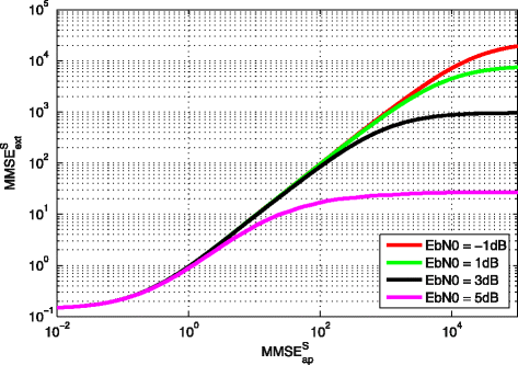

  

  Relationship between $\text {MMSE}_{\text {ext}}^{S}$ and $\text {MMSE}_{\text {ap}}^{S}$ for the sequential message passing with different $\frac {E_{b}}{N_{0}}$

• 2. With a large $\text {MMSE}_{\text {ap}}^{S}$, the higher $\frac {E_{b}}{N_{0}}$ is, the higher $\text {MMSE}_{\text {ext}}^{S}$ is. With the increasing of $\text {MMSE}_{\text {ap}}^{S}$, x(t−1) provides less amount of priori information for the prediction y(t), and the extrinsic information from channel decoder becomes dominant in the prediction of y(t). Then, the channel gains with different $\frac {E_{b}}{N_{0}}$ are seen.

• 3. When $\text {MMSE}_{\text {ap}}^{S}$ is around 1.0e −2, the values $\text {MMSE}_{\text {ext}}^{S}$ are flat. This arises because, based on the information from the time slots priori to t+1, the prediction of y(t) is not reliable since state dynamics n(t) and the noise of system observation w(t) are not predictable. This leads that the minimum value of $\text {MMSE}_{\text {ext}}^{S}$ is limited by the covariance matrix of n(t) and w(t), i.e., Σ _n and Σ _w , respectively.

Following the same idea of the EXIT chart and the MSE transfer chart for iterative channel decoding, we use the MSE transfer chart to evaluate the performance of BP-based sequential channel decoding and state estimation over mutiple time slots. In the MSE transfer chart, we have two curves: one is $\text {MMSE}_{\text {ap}}^{S,t}$ versus $\text {MMSE}_{\text {ext}}^{S,t}$, which is equivalent to the curve for $\text {MMSE}_{\text {ap}}^{S}$ versus $\text {MMSE}_{\text {ext}}^{S}$($\text {MMSE}_{\text {ap}}^{S}$ and $\text {MMSE}_{\text {ext}}^{S}$ at time slot t); the other is $\text {MMSE}_{\text {ext}}^{S,t+1}$ versus $\text {MMSE}_{\text {ap}}^{S,t+1}$, which is equivalent to the flipped curve for $\text {MMSE}_{\text {ap}}^{S}$ versus $\text {MMSE}_{\text {ext}}^{S}$($\text {MMSE}_{\text {ap}}^{S}$ and $\text {MMSE}_{\text {ext}}^{S}$ at time slot t+1).

The MSE transfer chart for $\frac {E_{b}}{N_{0}}=$5 dB is shown in Fig. 19. There is one crossing/convergence point between these two curves, which means that it is not a successful decoding from I _A =0 to I _A =1. The arrows with black color show the trace of the sequential message passing(starting from $\text {MMSE}_{\text {ap}}^{S}$=1.0e −2 at time slot t). We can see that trace moves toward the convergence point at time slot t+1 and t+2. The trace shows that even if we have perfect knowledge of y(t) at time slot t, the performance of state estimation degrades toward the crossing point after running a few time slots. The arrows with red color show the other trace (starting from $\text {MMSE}_{\text {ap}}^{S}$=1.0e + 5), at which there is no priori information from the prediction of y(t). Similarly, we can see the trace is moving toward the convergence point at time slot t+1,t+2,···. Different from the above, this trace shows that even though there is no priori information of y(t) at time slot t, the performance of state estimation is improved after running a few time slots, and finally, the gain reaches the convergence point.

Fig. 19

The MSE transfer chart for sequential channel decoding and state estimation: $\frac {E_{b}}{N_{0}}$=5 dB

Figure 20 illustrates the MSE transfer chart as $\frac {E_{b}}{N_{0}}=$3 dB with one crossing point at $\text {MMSE}_{\text {ap}}^{S,t}$=1.0e −0.15. In the range of [1.0e −0.15, 1.0e + 2], the gap between the curve ($\text {MMSE}_{\text {ap}}^{S,t}$ versus $\text {MMSE}_{\text {ext}}^{S,t}$) and the flipped curve ($\text {MMSE}_{\text {ext}}^{S,t+1}$ versus $\text {MMSE}_{\text {ap}}^{S,t+1}$) is very small. This means that the convergence speed is slow and it takes many time slots to converge to the convergence point when the state estimator has no priori information of y(t) at time slot t.

Fig. 20

The MSE transfer chart for sequential channel decoding and state estimation $\frac {E_{b}}{N_{0}}$=3 dB

Figure 21 shows the MSE transfer chart as $\frac {E_{b}}{N_{0}}=$1 dB with one crossing point at $\text {MMSE}_{\text {ap}}^{S,t}$=1.0e −0.15. Note that after the crossing point the curve ($\text {MMSE}_{\text {ap}}^{S,t}$ versus $\text {MMSE}_{\text {ext}}^{S,t}$) almost overlaps with the flipped curve ($\text {MMSE}_{\text {ext}}^{S,t+1}$ versus $\text {MMSE}_{\text {ap}}^{S,t+1}$). This shows two conditions when the state estimator has no priori information of y(t) at time slot t: one is that it will gain a high MSE and cannot coverage to the crossing point; the other is that it will take many time slots to converge to the crossing point. Compared with previous two results, for $\frac {E_{b}}{N_{0}}$=1 dB, the MSEs of estimating x(t) and y(t) are much higher than that for $\frac {E_{b}}{N_{0}}$ equals to 3 and 5 dB. Similar results go with the case when $\frac {E_{b}}{N_{0}}=-$1 dB.

Fig. 21

The MSE transfer chart for sequential channel decoding and state estimation $\frac {E_{b}}{N_{0}}$=1 dB

6.3 Performance analysis for iterative channel decoding and state estimation

In this section, we show how to use the proposed MSE transfer chart to evaluate the performance of BP-based iterative channel decoding and state estimation within two time slots. As we stated, the node x(t−1) and the node y(t) provide the same amount of information in the context of information theory. From this point, the priori information at the node y(t), as same as the node x(t−1), will be $\pi _{\mathbf {x}(t-1), \mathbf {x}(t)}(\mathbf {x}(t-1))= \mathcal {N}(\mathbf {x}_{t-1}, \mathbf {x}_{\pi _{x}, t-1}, P_{\pi _{x}, t-1})$ with $\mathbf {x}_{\pi _{x}, t-1}=\mathbf {0}$ and $P_{\pi _{x}, t-1}=\text {MMSE}_{\text {ap}}^{t-1,x}\mathbf {I}_{k}$.

With the priori information as an initial input for iterative decoding, the gains of $\text {MMSE}_{\text {ext}}^{t}$(based on $\text {MMSE}_{\text {ap}}^{t}$) with different $\text {MMSE}_{\text {ap}}^{t-1,x}$ and $\frac {E_{b}}{N_{0}}$=5 dB are illustrated in Fig. 22, and from this figure, we have the following observations:

• 1. With the same $\text {MMSE}_{\text {ap}}^{t-1,x}$, the higher $\text {MMSE}_{\text {ap}}^{t}$ is, the lower gain of $\text {MMSE}_{\text {ext}}^{t}$ can be obtained from $\text {MMSE}_{\text {ap}}^{t}$.

  Fig. 22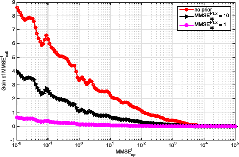

  

  Gain of $\text {MMSE}_{\text {ext}}^{t}$ from $\text {MMSE}_{\text {ap}}^{t}$ with different $\text {MMSE}_{\text {ap}}^{t-1, x}$ and $\frac {E_{b}}{N_{0}}$=5 dB

• 2. The higher the $\text {MMSE}_{\text {ap}}^{t-1,x}$ is, the higher gain of $\text {MMSE}_{\text {ext}}^{t}$ can be obtained from $\text {MMSE}_{\text {ap}}^{t}$. This exists because the prediction of y(t+1) is contributed by both priori information from x(t−1) and the extrinsic information from the channel decoder at time slot t. When $\text {MMSE}_{\text {ap}}^{t-1,x}$ is small, the information from x(t−1) is dominant in predicting y(t+1). Although the prediction of y(t) can increase the amount of extrinsic information from channel decoder at time slot t, it cannot contribute much to the gain of $\text {MMSE}_{\text {ext}}^{t}$ as the priori information from x(t−1) is dominant.

Following the same idea, the gain of $\text {MMSE}_{\text {ext}}^{t+1}$ (based on $\text {MMSE}_{\text {ap}}^{t+1}$) is obtained and shown in Fig. 23. Similar observations as above are obtained:

• 1. With the same $\text {MMSE}_{\text {ap}}^{t-1,x}$, the higher $\text {MMSE}_{\text {ap}}^{t+1}$ is, the lower gain of $\text {MMSE}_{\text {ext}}^{t+1}$ can be obtained from $\text {MMSE}_{\text {ap}}^{t}$.

  Fig. 23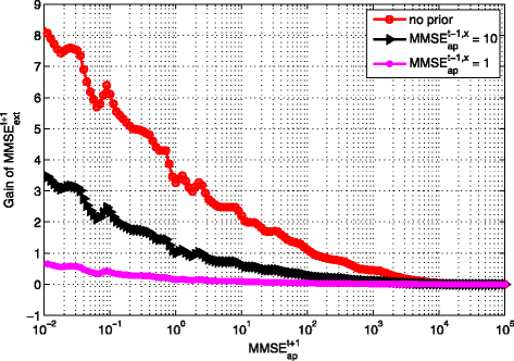

  

  Gain of $\text {MMSE}_{\text {ext}}^{t+1}$ from $\text {MMSE}_{\text {ap}}^{t+1}$ with different $\text {MMSE}_{\text {ap}}^{t-1,x}$ and $\frac {E_{b}}{N_{0}}$=5 dB

• 2. The higher the $\text {MMSE}_{\text {ap}}^{t-1,x}$ is, the higher gain of $\text {MMSE}_{\text {ext}}^{t+1}$ can be obtained from $\text {MMSE}_{\text {ap}}^{t+1}$.

Then, the MSE transfer chart for BP-based iterative channel decoding and state estimation is formed by the curve ($\text {MMSE}_{\text {ap}}^{t}$ versus $\text {MMSE}_{\text {ext}}^{t}$) and the flipped curve ($\text {MMSE}_{\text {ap}}^{t+1}$ versus $\text {MMSE}_{\text {ext}}^{t+1}$), and the results with different $\text {MMSE}_{\text {ap}}^{t-1,x}$ and $\frac {E_{b}}{N_{0}}=$5 dB are shown in Fig. 24. In the following, we try to explain our observations based on the case where no priori information are considered.

• 1. BP-based iterative channel decoding can decrease $\text {MMSE}_{\text {ext}}^{t}$ and help improve the estimation of x(t+1). The values of the crossing point between the curve ($\text {MMSE}_{\text {ap}}^{t}$ versus $\text {MMSE}_{\text {ext}}^{t}$) and the flipped curve ($\text {MMSE}_{\text {ap}}^{t+1}$ versus $\text {MMSE}_{\text {ext}}^{t+1}$) for $\text {MMSE}_{\text {ap}}^{t}$ and $\text {MMSE}_{\text {ext}}^{t}$ are 1.0e + 1.33 and 1.0e + 1.25, respectively, while the values of $\text {MMSE}_{\text {ap}}^{t}$ and $\text {MMSE}_{\text {ext}}^{t}$ with no priori information are 1.0e + 5 and 1.0e + 1.43, respectively. Therefore, the total gain of $\text {MMSE}_{\text {ext}}^{t}$ for BP-based iterative channel decoding and state estimation is 10∗(1.43−1.25)=1.8 dB.

  Fig. 24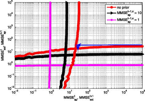

  

  MSE-based transfer chart for iterative channel decoding and system state estimation with different $\text {MMSE}_{\text {ap}}^{t-1,x}$ and $\frac {E_{b}}{N_{0}}$=5 dB

• 2. The gain of $\text {MMSE}_{\text {ext}}^{t}$ with only three steps is close to the gain of $\text {MMSE}_{\text {ext}}^{t}$ at the convergence point. The trace of BP-based iterative channel decoding and state estimation with the mentioned three steps is shown by the arrows with blue color in the figure, and the details are listed as below:

  • 1) From y(t) to y(t+1): As there is no priori information, the starting point is $\text {MMSE}_{\text {ap}}^{t}$ with the value of 1.0e + 5, and the corresponding value of $\text {MMSE}_{\text {ext}}^{t}$ is 1.0e + 1.43.

  • 2) From y(t+1) to y(t): We have $\text {MMSE}_{\text {ap}}^{t+1}$ with the value of 1.0e + 1.43, and the corresponding value of $\text {MMSE}_{\text {ext}}^{t+1}$ is 1.0e + 1.34.

  • 3) From y(t) to y(t+1): We have $\text {MMSE}_{\text {ap}}^{t}$ with the value of 1.0e + 1.34, and the corresponding value of $\text {MMSE}_{\text {ext}}^{t}$ is 1.0e + 1.255. Compared with step (1), 10∗(1.43−1.255)=1.75 dB is obtained for $\text {MMSE}_{\text {ext}}^{t}$ while it is 1.8 dB for $\text {MMSE}_{\text {ext}}^{t}$ from convergence point. Thus, the gain loss for BP-based iterative channel decoding and state estimation with these three steps is just 1.8−1.75=0.05 dB.

  In summary, we can implement BP-based iterative channel decoding and state estimation with above three steps to obtain the gain of $\text {MMSE}_{\text {ext}}^{t}$, which is close to the gain at convergence point.

Note that when $\text {MMSE}_{\text {ap}}^{t-1,x}$ equals to 1 or 10, the BP-based iterative channel decoding and state estimation scheme cannot improve the performance of state estimation. This is because with a small $\text {MMSE}_{\text {ap}}^{t-1,x}$ the priori information from x(t) is dominant in estimating y(t+1), which leads that the prediction of y(t) in channel decoder at time slot t is negligible in predicting y(t+1).

The MSE transfer charts for $\frac {E_{b}}{N_{0}}=3$ and 1 dB have similar observations as that for $\frac {E_{b}}{N_{0}}=$5 dB, so we will not list the results here.

6.4 Performance analysis for Kalman filtering-based heuristic approach

Similarly, by utilizing the redundancy of system dynamics, a Kalman filtering-based heuristic approach is evaluated in this section. In the Kalman filtering-based heuristic approach, the prediction of y(t) based on Kalman filtering is used as the priori information for b(t), and instead of using only the extrinsic information of the channel decoder to obtain a soft estimation of y(t), the total information including both the priori information and the extrinsic information generated by the channel decoder is used to obtain a hard estimation of y(t).

The corresponding framework used for the Kalman filtering-based heuristic approach is similar to the BP-based channel decoding and state estimation as shown in Fig. 12 (b). The priori information from y(t) is modeled with $\mathbf {S}_{\pi, t}=\text {MMSE}_{\text {ap}}^{Y}\mathbf {I}_{K}$, and the priori information for b(t) is represented by mutual information I _A . Finally, the total information from the channel decoder for estimating of b(t) is modeled by $\text {MMSE}^{B}_{\text {tot}}$, which means the MMSE of estimating b(t) based on the total information including both the priori information and the extrinsic information from the channel decoder.

Figure 25 illustrates the relationship between $\text {MMSE}_{\text {ap}}^{Y}$ and $\text {MMSE}_{\text {tot}}^{Y}$. The gains of $\text {MMSE}_{\text {tot}}^{Y}$ with different $\text {MMSE}_{\text {ap}}^{Y}$ and $\frac {E_{b}}{N_{0}}$ are shown in Fig. 26, which are further improved comparing to Fig. 17.

Fig. 25

$\text {MMSE}_{\text {tot}}^{Y}$ with different $\text {MMSE}_{\text {ap}}^{Y}$ and $\frac {E_{b}}{N_{0}}$

Fig. 26

Gain of $\text {MMSE}_{\text {tot}}^{Y}$ with different $\text {MMSE}_{\text {ap}}^{Y}$ and $\frac {E_{b}}{N_{0}}$

7 Conclusions

We propose to use the MSE transfer chart to evaluate the performance of BP-based channel decoding and state estimation. We focus on two models, the BP-based sequential processing model and the BP-based iterative processing model, for channel decoding and state estimation. The former can be used to evaluate the performance of sequential processing over multiple time slots, and the latter can be used to evaluate the performance of iterative processing within two time slots. The numerical results show by utilizing the MSE transfer chart the proposed channel decoding and state estimation algorithm can decrease the MSE and improve performance of channel decoding and state estimation. Specifically, a total 1.75 dB gain can be earned through three-step BP-based iterative channel decoding and state estimation process when no prior information is given.

References

S Gong, H Li, L Lai, RC Qiu, in 2011 IEEE International Conference on Communications (ICC). Decoding the’nature encoded’messages for distributed energy generation control in microgrid (IEEEKyoto, 2011), pp. 1–5.
H Li, Communications for control in cyber physical systems: theory, design and applications in smart grids (Morgan Kaufmann, Cambridge, 2016).
S ten Brink, Convergence of iterative decoding. Electron. Lett.35(10), 806–808 (1999).
S Ten Brink, in Proceedings of 3rd IEEE/ITG Conference on Source and Channel Coding, Munich, Germany. Iterative decoding trajectories of parallel concatenated codes, (2000), pp. 75–80.
S Ten Brink, Convergence behavior of iteratively decoded parallel concatenated codes. IEEE Trans. Commun.49(10), 1727–1737 (2001).
M El-Hajjar, L Hanzo, Exit charts for system design and analysis. IEEE Commun. Surveys Tutorials. 16(1), 127–153 (2013).
K Bhattad, KR Narayanan, An MSE-based transfer chart for analyzing iterative decoding schemes using a Gaussian approximation. IEEE Trans. Inf. Theory.53(1), 22–38 (2007).
A Ashikhmin, G Kramer, S ten Brink, Extrinsic information transfer functions: model and erasure channel properties. IEEE Trans. Inf. Theory. 50(11), 2657–2673 (2004).
D Guo, S Shamai, Verdu, Ś, Mutual information and minimum mean-square error in Gaussian channels. IEEE Trans. Inf. Theory. 51(4), 1261–1282 (2005).
M Fu, CE de Souza, State estimation for linear discrete-time systems using quantized measurements. Automatica. 45(12), 2937–2945 (2009).
S Yüksel, Bas, Ţ,ar, Stochastic networked control systems. AMC. 10:, 12 (2013).
L Li, H Li, in Global Communications Conference (GLOBECOM), 2016 IEEE. Dynamic state aware source coding for networked control in cyber-physical systems (IEEEWashington, DC, 2016), pp. 1–6.
S Yüksel, On stochastic stability of a class of non-Markovian processes and applications in quantization. SIAM J. Control. Optim.55(2), 1241–1260 (2017).
N Ramzan, S Wan, E Izquierdo, Joint source-channel coding for wavelet-based scalable video transmission using an adaptive turbo code. EURASIP J. Image Video Process.2007(1), 1–12 (2007).
V Kostina, Verdu, Ś, Lossy joint source-channel coding in the finite blocklength regime. IEEE Trans. Inf. Theory. 59(5), 2545–2575 (2013).
H Wu, L Wang, S Hong, J He, Performance of joint source-channel coding based on protograph LDPC codes over Rayleigh fading channels. IEEE Commun. Lett.18(4), 652–655 (2014).
X He, X Zhou, P Komulainen, M Juntti, T Matsumoto, A lower bound analysis of hamming distortion for a binary ceo problem with joint source-channel coding. IEEE Trans. Commun.64(1), 343–353 (2016).
Y Wang, M Qin, KR Narayanan, A Jiang, Z Bandic, in Global Communications Conference (GLOBECOM), 2016 IEEE. Joint Source-Channel Decoding of Polar Codes for Language-Based Sources (IEEEWashington, DC, 2016), pp. 1–6.
V Kostina, Y Polyanskiy, S Verd, Joint source-channel coding with feedback. IEEE Trans. Inf. Theory. 63(6), 3502–3515 (2017).
L Yin, J Lu, Y Wu, in Communication Systems, 2002. ICCS 2002. The 8th International Conference On, 1. LDPC-based joint source-channel coding scheme for multimedia communications (IEEESingapore, 2002), pp. 337–341.
J Garcia-Frias, W Zhong, LDPC codes for compression of multi-terminal sources with hidden Markov correlation. IEEE Commun. Lett. 7(3), 115–117 (2003).
W Zhong, Y Zhao, J Garcia-Frias, in Conference Record of the Thirty-Seventh Asilomar Conference on Signals, Systems and Computers. Turbo-like codes for distributed joint source-channel coding of correlated senders in multiple access channels (IEEEPacific Grove, 2003), pp. 840–844.
Z Mei, L Wu, Joint source-channel decoding of Huffman codes with LDPC codes. J Electron (China). 23(6), 806–809 (2006).
X Pan, A Cuhadar, AH Banihashemi, Combined source and channel coding with JPEG2000 and rate-compatible low-density parity-check codes. IEEE Trans. Signal Process.54(3), 1160–1164 (2006).
L Pu, Z Wu, A Bilgin, MW Marcellin, B Vasic, LDPC-based iterative joint source-channel decoding for JPEG2000. IEEE Trans. Image Process.16(2), 577–581 (2007).
M Fresia, F Perez-Cruz, HV Poor, S Verdu, Joint source and channel coding. IEEE Signal Proc. Mag.27(6), 104–113 (2010).
E Koken, E Tuncel, Joint source-channel coding for broadcasting correlated sources. IEEE Trans. Commun. (2017).
B Girod, AM Aaron, S Rane, D Rebollo-Monedero, Distributed video coding. Proc. IEEE. 93(1), 71–83 (2005).
Y Zhao, J Garcia-Frias, Joint estimation and compression of correlated nonbinary sources using punctured turbo codes. IEEE Trans. Commun.53(3), 385–390 (2005).
R Gallager, Low-density parity-check codes. IRE Trans. Informa. Theory. 8(1), 21–28 (1962).
J Pearl, Probabilistic Reasoning in Intelligent Systems: Networks of Plausible Inference (Morgan Kaufmann Publishers Inc., San Francisco, 1988).
Acknowledgements
The authors would like to thank the support of National Science Foundation under grants ECCS-1407679, CNS-1525226, CNS-1525418, and CNS-1543830.
Author information
Authors and Affiliations
Contributions
HL conceived the Brainbow strategies for this work. JBS and HL supervised the project. SG built the initial constructs and LL validated them, analyzed the data, and wrote the paper. All authors read and approved the final manuscript.
Corresponding author
Ethics declarations
Competing interests
The authors declare that they have no competing interests.
Publisher’s Note
Springer Nature remains neutral with regard to jurisdictional claims in published maps and institutional affiliations.
Rights and permissions
Open Access This article is distributed under the terms of the Creative Commons Attribution 4.0 International License (http://creativecommons.org/licenses/by/4.0/), which permits unrestricted use, distribution, and reproduction in any medium, provided you give appropriate credit to the original author(s) and the source, provide a link to the Creative Commons license, and indicate if changes were made.
About this article
Cite this article
Li, L., Gong, S., Song, J.B. et al. Performance analysis on joint channel decoding and state estimation in cyber-physical systems. J Wireless Com Network 2017, 158 (2017). https://doi.org/10.1186/s13638-017-0943-y
Received:
Accepted:
Published:
DOI: https://doi.org/10.1186/s13638-017-0943-y