Modeling of Real Time Kinematics localization error for use in 5G networks

Abstract

In 5G networks information about localization of a user equipment (UE) can be used not only for emergency calls or location-based services, but also for the network optimization applications, e.g., network management or dynamic spectrum access by using Radio Environment Maps (REM). However, some of these applications require much better localization accuracy than currently available in 4G systems. One promising localization method is Global Navigation Satellite System (GNSS)-based Real-Time Kinematics (RTK). While the signal received from satellites is the same as in traditional GNSS, a new reception method utilizing real-time data from a nearby reference station (e.g., 5G base station) results in cm-level positioning accuracy. The aim of this paper is to obtain a model of the RTK localization error for smartphone-grade GNSS antenna under open-sky conditions, that can be used in 5G network simulators. First, a tutorial-style overview of RTK positioning, and satellite orbits prediction is provided. Next, an RTK localization simulator is implemented utilizing GNSS satellites constellations. Results are investigated statistically to provide a simple, yet accurate RTK localization error framework, which is based on two Gauss-Markov process generators parametrized by visible satellites geometry, UE motion, and UE-satellite distance error variance.

1 Introduction

The development of localization methods in cellular networks started with the formulation of the enhanced 911 (E911) location requirements by the Federal Communications Commission (FCC) of the USA in the 1990s [1]. The aim of the E911 requirements were to locate user equipment (UE) emergency calls with the root-mean square error (RMSE) of 125 m in 67% of all cases [1]. In cellular networks from 2G to 4G, firstly standardization effort was put into fulfil government requirements. With the networks development UE localization information began to be attractive for operators from a commercial point of view, resulting in introduction of location-based services (e.g. social networking, advertising) [1].

5G networks come with a set of new use cases where UE localization information is necessary, not only for emergency and user-plane applications, but also for Intelligent Transportation Systems Aerial Vehicles or Industrial Applications [2]. Moreover in 5G systems localization, data will be utilized for network optimization applications such as self-organizing networks (SON), network management, or dynamic spectrum access (DSA) [1].

Implementation of the mentioned network optimization applications may be based on the Radio Environment Maps (REMs) for both SON [3] and DSA [4]. REM can be understood as a real-time model of the real-world radio environment using multi-domain information (e.g., available radio links, wireless channel parameters) [5]. However, the implementation of REM requires accurate and robust localization information, firstly during data acquisition, and secondly when serving REM users. Localization can be achieved either by means of trilateration [6–8], triangulation [9], or fingerprinting [10]. However, the most suitable localization method for REM under outdoor and open-sky conditions is the Real Time Kinematics (RTK) [11] which is based on Global Navigation Satellite System (GNSS). It provides centimeter-level accuracy based on standard satellite-based GNSS signal while requiring constant connection to a reference station of known coordinates, e.g., 5G base station (BS). Although the localization error of the conventional GNSS is well investigated [12], there is no RTK error model that takes into account the localization error as a function of daytime and geographical localization.

The aim of this paper is to study on the RTK localization error for smartphone-grade antenna under open-sky conditions, assuming line-of-sight (LoS) propagation between UE and each of the satellites. For better understanding of the RTK localization approach, detailed tutorial-style mathematical description is also provided. Based on simulations and statistical analysis important factors are extracted and a simplified yet accurate framework for the generation of RTK localization error is proposed. The framework takes into account UE motion, UE location and time of a day influencing geometry of visible satellites. One additional parameter is the cutoff angle allowing to consider only GNSS satellites exceeding given elevation above horizon. This allows for mimicking RTK operation in the urban environment where buildings block LoS propagation between some satellites and an UE. The resultant error both follows the proper distribution and is time continuous. The proposed model is of high importance when simulating 5G systems that utilize REM technology in outdoor environment with relatively low altitude buildings. Step-by-step description of the proposed algorithm is presented to simplify its implementation.

This paper is organized as follows: related work is discussed in Section 2. Section 3 provides brief description of REM concept and highlights some of the REMs applications where accurate localization may be required. Section 4 introduces the concept of RTK in relation to the conventional GNSS localization. Section 5 describes mathematical models of RTK, almanac-based satellites orbits prediction, and theory related with Gauss-Markov process including its generation with autoregressive model. Section 6 discusses the simulation results of the RTK localization error. The simplified framework for generation of RTK localization error under open-sky conditions is proposed in Section 7. Conclusions are formulated in Section 8.

2 Related work

As mentioned there are various ways to obtain user position. Some of them utilize trilateration, e.g., Observed Time Difference of Arrival (OTDoA) defined for cellular networks in LTE Positioning Protocol (LPP) [6], 802.15.4a ultra wide band (UWB) [7], or different implementations of GNSS, e.g., Global Positioning System (GPS) or Galileo [8]. Other ones, may use triangulation. This approach requires accurate Angle of Arrival (AoA) measurements, thus it is expected to be used in 5G systems utilizing massive MIMO (M-MIMO) technology [9]. Another interesting localization technique is utilization of radio frequency pattern matching (RFPM), called also fingerprinting. User position is estimated by comparing measured value (e.g., received signal strength (RSS)), with the fingerprint (previously measured RSS, tagged with geographical localization) from database. User position is the localization tag of the best matching fingerprint [10]. Fingerprinting is not explicitly defined in LPP; however, there are some works describing its implementation on the basis of the LTE positioning infrastructure [13, 14].

On the other hand RTK is defined in LPP [6] and foreseen for 5G networks [15]. The RTK method is mostly useful when REM is utilized in 5G network under outdoor conditions. With its centimeter-level accuracy it is currently widely used in geodesy or agriculture. Furthermore, it has been shown that RTK may be available for smart phones and provide cm-level accuracy in the open-sky conditions [16]. However, its performance can be degraded in urban environment, e.g., due to the cycle-slips phenomenon [17, 18].

While considering localization techniques as important features of the 5G systems, questions arise on the reliability of acquired localization data and the influence of the localization error on the network performance. The localization error of the conventional GNSS can be modeled as a bivariate normal distribution with x (e.g., North-South) and y(e.g., East-West) direction errors being uncorrelated [12]. In the case of RTK such a model, suitable, e.g., for 5G network simulations, is not available. In [19], authors analyzed localization error components of the RTK variant utilizing several cooperating base stations arranged in network, i.e. network RTK (NRTK). The final localization error obtained on the basis of the mathematical models and raw measurements is given only in terms of root-mean square (RMS). However, no information could be found about distribution, influence of satellites constellation or correlation of error in time. Studies in [20] are focused on the impact of the air humidity and sky obstruction on RTK localization error, but with no proposal of global RTK error model.

In [21], an error model is proposed, but its parameters are obtained only on the basis of the raw RTK measurements related to specific geographical localization. Also, the impact of the visible satellites geometry on RTK localization error was not taken into account.

3 5G radio environment maps

As it was mentioned in the Section 1, REMs are going to be a significant part of the future 5G networks. Their main aim is to improve the efficiency of the network and radio resources management. This section will firstly briefly describe REM concept and secondly discuss some of the 5G REMs applications, where accurate localization can be required.

3.1 REM concept

REM can be described as a live-changing model of a real-world radio environment using multi-domain information [5]. REM stores and processes information to support prediction and intelligent network management. Data stored in REM can be divided into long-term information (e.g., base station antenna parameters, local country law restrictions) and short-term information (e.g., available radio links, wireless channel parameters) [22].

Figure 1 depicts an example structure realization of REM as suggested in [23]. The context information tagged with localization and time is provided by so-called measurement capable devices (MCDs), e.g., UEs or BSs. Capturing the data from the MCDs is managed by the so-called REM acquisition module, and the information is further stored in REM storage structure. REM users sends service requests tagged with its current localization to the REM manager. REM manager is an intelligent part of the REM responsible for processing data from REM storage module and handling REM users requests.

Fig. 1

The example REM structure

3.2 Possible RTK applications in 5G REMs

As depicted in Fig. 1, REMs require localization information firstly to tag MCDs measurements with location, and secondly when REM user requests service from REM manager. There are many applications of 5G REMs which require accurate positioning, e.g.,

• Interference coordination: [24] where power density maps allow to perform interference coordination between users in a network.

• M-MIMO [25] where a database of the UEs AoAs related to the localization is proposed to manage Spatial Division Multiple Access (SDMA) in MIMO networks.

• Location-based protocols in vehicular networks [26] where REM provides location-specific transmission parameters for each vehicle.

In the spectrum sensing and M-MIMO, an accurate localization method like RTK can reduce errors related to the database measurement grid. This can allow for more accurate information especially in higher frequencies. In the case of location-based protocols in vehicular networks RTK can be utilized for much more precise definition of transmission areas.

4 GNSS localization

This section provides a brief description of the conventional positioning with GNSS, and later introduces the concept of RTK. In addition some features of RTK, e.g., UE-satellite range error, energy consumption, are discussed in relation to the conventional GNSS.

4.1 Conventional GNSS

A GNSS receiver uses the trilateration method to compute its position based on the distances measured to at least four satellites of known coordinates. A conventional GNSS receiver computes the distance between a UE and a satellite by obtaining the time offset between spread spectrum code transmitted by the satellite and a local code replica (code phase measurements). A chipping rate for basic civil L1 GPS signal is 1.023 Mcps. Even though the received signal is sampled at frequencies higher than the chip rate, due to, e.g., the multipath propagation and the receiver noise the UE-satellite range error equals for the state of art receivers about 1 m [8]. Additional source of error is the propagation through the troposphere and the ionosphere. The signal propagation speed and direction is changing while passing through these atmosphere layers. Moreover, non-perfect clocks synchronization, especially caused by relatively low quality UE’s local oscillator, causes the satellite-UE clock offsets. These are another sources of propagation error causing the final UE-satellite range error for the stand-alone single-frequency receiver to equal around 6 m [8].

4.2 RTK

Real-Time Kinematics refers to the obtaining position estimation of moving UE in real time (i.e. without additional post-processing), with the help of a reference station, and on the basis of the carrier phase measurements [20]. Similarly, as in concventional GNSS receiver, RTK also provides UE position estimate based on the trilateration method. The difference lies in the method for obtaining the distance between the UE and the satellite. While conventional GNSS receiver utilizes code phase measurements, in RTK, the UE-satellite range computation is based on the phase difference between the carrier signal received from the satellite and the local carrier replica (carrier phase measurements). Second difference in relation to the conventional GNSS is taking advantage of the so-called relative positioning, where a reference station of known coordinates is utilized, as shown in Fig. 2. The position of UE in relation to the reference station position is obtained with the help of assistance data provided by the reference station (e.g., its localization and raw carrier phase measurements data) [8].

Fig. 2

Concept of the reference station providing assistance data (mainly it’s raw measurements) to the UE

The UE-satellite range influences the received signal phase which is normalized to a carrier wavelength. The distance between satellite and UE is presented as the sum of an integer and a fractional number of carrier wavelengths. By the solving proper equation, the receiver can find this integer number of wavelengths, and thus solve the so-called “integer ambiguity” shown in Fig. 3. At the same time, UE position approximating mostly the received carrier phase from all visible GNSS satellites is established. The fractional phase ϕ(t) estimate allows for tracking UE position with sub-wavelength accuracy. The RTK receiver initialization time which is referred to as time to ambiguity resolution (TAR) [16], corresponds to the time necessary for resolution of the integer ambiguities. The maximum error in carrier phase measurement is below 1 carrier wavelength which for the L1 GPS signal frequency, i.e., 1575.42 MHz, equals about 19 cm [8].

Fig. 3

Comparison between code and carrier phase measurements

The carrier phase measurements are affected by the same types of phenomena like code phase measurements: multipath propagation, receiver noise, atmospheric propagation errors, and satellite and UE clock biases. However, thanks to the relative positioning, atmospheric propagation errors, and clock biases may be canceled out as discussed in Section 5.1. UE-satellite range error for carrier phase measurements is typically in the range from 0.5 to 1 cm and is mainly caused by the multipath propagation of GNSS signals, while best UE-satellite range accuracy achieved using code phase measurements is about 1 m [8]. Such high RTK performance is achieved at the cost of increased power consumption in the order of 100 mW as compared to about 10 mW for code phase measurements [16]. Additionally, continuous raw measurements data from the reference station (e.q., 5G BS) have to be provided to the UE. However, such a mechanism is already standardized in LPP [6].

5 RTK positioning and error

A general RTK description from the previous section can be extended to form a mathematical model. In this section, the state of the art about RTK positioning, and the satellite orbits prediction are presented in a tutorial-style to simplify implementation by interested readers. Both the utilization of the autoregressive model for UE-satellite distance error modeling, and the RTK error estimation simulation environment are proposed by the authors.

The phase of a GPS signal is measured as the number of wavelength cycles in $\frac {rad}{2\pi }$¹ i.e., a standard phase changing from 0 to 2π over single carrier period can be divided by 2π to form values from 0 to 1. Denoting $f(\hat t)$ as an instantaneous GNSS signal frequency at time instant τ, the signal phase at the time t, φ(t), depends on the phase at time instance t₀ as [8]:

$$ \varphi(t) = \varphi(t_{0}) + \int_{t_{0}}^{t} f(\hat t) d\hat t. $$

(1)

Assuming perfect clocks measuring time epochs t₀ and t, and f(τ) being constant, f(τ)≈f₀, for short time interval, we can write

$$ \varphi(t) = \varphi(t_{0}) + f_{0} \cdot (t-t_{0}). $$

(2)

The signal phase changes linearly and proportionally to the time difference. If the GNSS signal travels from satellite to UE, a delay of Δt is introduced by the propagation. At the time, instant t the GNSS receiver will detect phase

$$ \varphi(t-\Delta t) = \varphi(t) - f_{0}\Delta t. $$

(3)

The satellite-receiver carrier phase distance measurement can be now expressed as a measured fraction of the wavelength cycle and an unknown integer number of full cycles (integer ambiguity) [8]:

$$ \phi(t) = \varphi_{r}(t) - \varphi_{s}(t-\Delta t) + N, $$

(4)

where N is an integer ambiguity, φ_r(t) is the local carrier replica phase, and φ_s(t−Δt) is the phase of the carrier received from satellite delayed by the propagation time Δt. When the receiver acquires a phase lock with the satellite signal, then φ_r(t)=φ_s(t). Based on Eq. (3), Eq. (4) can be expressed as

$$ \phi(t) = f\Delta t + N = \frac{r}{\lambda} + N, $$

(5)

where r is the satellite-receiver distance in meters and λ is the carrier wavelength in meters. However, the measured phase is distorted by the satellite and the receiver clock biases, δt_s, δt_r, caused by the non-ideal synchronization between satellites and receivers clocks. Secondly, the measured phase suffers from the troposphere propagation error (T, in meters) and the ionosphere propagation error (J, in meters). Moreover, the receiver noise and the multipath propagation introduces an additional error ε, so that the final measured carrier phase can be expressed as [8]

$$ \phi = \frac{r + J + T}{\lambda} + \frac{c}{\lambda}(\delta t_{r} - \delta t_{s}) + \epsilon + N. $$

(6)

Errors from the above equation can be split into the slow and fast varying. Slow varying errors are atmospheric delays (J, T) and clock biases (δt_s, δt_r), which can persist for tens of minutes [8]. Fast varying errors are related to multipath propagation, and receiver noise (ε). They are claimed to be zero mean i.e. E[ε]=0, and uncorrelated between measurements related to the different satellites i.e. E[εⁱε^j]=0, for i≠j, and ${ E}[\epsilon ^{i} \epsilon ^{j}] = \sigma ^{2}_{\phi }$, for i=j. Indices i, j denote satellite i, and j respectively [8].

5.1 Relative positioning

To cancel out propagation errors (T, J) and clock biases (δt_s,δt_r), the RTK is taking advantage of the so-called relative positioning. The position of a user receiver is estimated on the basis of its own measurements and the raw measurements from a reference base station of known coordinates (possibly a 5G base station). The position is estimated as an offset to the reference station coordinates [8].

5.1.1 Single difference

A general carrier phase measurement formula is given by (6). Let us denote the phase of the ith satellite signal measured at the UE as $\phi _{u}^{i}$, and the phase of the ith satellite signal measured at the reference station as $\phi _{r}^{i}$. After subtracting Eq. (6), related with UE and reference station we get

$$\begin{array}{*{20}l} {}\phi_{ur}^{i} &= \phi_{u}^{i} - \phi_{r}^{i} = \lambda^{-1} \left[\left(r_{u}^{i} - r_{r}^{i}\right) - \left(J_{u}^{i} - J_{r}^{i}\right) + \left(T_{u}^{i} - T_{r}^{i}\right)\right] \\ &\quad +\frac{c}{\lambda}\cdot (\delta t_{u} \,-\, \delta t_{r} \,+\, \delta t^{i}_{s} - \delta t^{i}_{s}) + (N_{u}^{i} - N_{r}^{i}) \!+ (\epsilon_{u}^{i} \,-\, \epsilon_{r}^{i}). \end{array} $$

(7)

When the UE is close enough to the reference station i.e., less than 5 km of distance [16], the ionosphere and troposphere propagation errors are proven to be the same ($J_{u}^{i} - J_{r}^{i}=0$ and $T_{u}^{i} - T_{r}^{i}=0$) [16], which can simplify (7) to

$$ \phi_{ur}^{i} = \lambda^{-1}r_{ur}^{i} + \frac{c}{\lambda} \cdot \delta t_{ur} + N_{ur}^{i} + \epsilon_{ur}^{i}, $$

(8)

where $(\bullet)_{ur}^{i} = (\bullet)_{u}^{i} - (\bullet)_{r}^{i}$.

5.1.2 Double difference

While atmospheric errors and satellite clock bias are canceled out by the single difference operation, UE and reference station clock biases (δt_ur) may be canceled out by double difference. Having single difference related to the ith satellite ($\phi _{ur}^{i}$), and single difference related to the jth satellite ($\phi _{ur}^{j}$), we can subtract them to get double difference [8]:

$$ {{}\begin{aligned} \phi_{ur}^{ij} &= \phi_{ur}^{i} - \phi_{ur}^{j} = \lambda^{-1}\left(r_{ur}^{i} - r_{ur}^{j}\right) + \frac{c}{\lambda} \cdot (\delta t_{ur} - \delta t_{ur})\\ &\quad +\!\left(N_{ur}^{i} - N_{ur}^{j}\right)\! +\! \left(\epsilon_{ur}^{i} - \epsilon_{ur}^{j}\right) = \lambda^{-1} r_{ur}^{ij} + N_{ur}^{ij} + \epsilon_{ur}^{ij}, \end{aligned}} $$

(9)

where $(\bullet)_{ur}^{ij} = (\bullet)_{ur}^{i} - (\bullet)_{ur}^{j}$.

It can be observed that the result of double difference operation is affected only by an error caused by receiver noise and multipath propagation $\epsilon _{ur}^{ij}$. Studies show that the dominant distortion is introduced by the multipath propagation. While receiver noise introduces about 1–2 mm rms error, in the UE-satellite range the UE-satellite rms range error caused by combined receiver noise and multipath propagation varies from 0.5 to 1 cm [8]. UE position estimation process utilizes a set of double difference Eq. (9) to estimate integer ambiguities $(N_{ur}^{ij})$ and obtain final UE position.

5.1.3 Double difference correlations

As already mentioned fast varying errors of the carrier phase measurement between UE and satellite ($\epsilon _{u}^{i}$ in Eq. (7)) are uncorrelated and have the same variance and zero mean. The undifferenced measurements error covariance matrix may be expressed as

$$ {\mathbf R} = E\left[[\boldsymbol{\phi_{u}}-E[\boldsymbol{\phi_{u}}]]\left[\boldsymbol{\phi_{u}}-E[\boldsymbol{\phi_{u}}]\right]^{H}\right] = E\left[\boldsymbol{\epsilon_{u}}\boldsymbol{\epsilon_{u}}^{H}\right], $$

(10)

where $\boldsymbol {\phi _{u}} = [\phi _{u}^{1}, \phi _{u}^{2}, \hdots, \phi _{u}^{K}]^{T}$, $\boldsymbol {\epsilon _{u}} = [\epsilon _{u}^{1}, \epsilon _{u}^{2}, \hdots, \epsilon _{u}^{K}]^{T}$ and H denotes Hermitian transpose. After taking into account our assumptions, it can be shown that, Eq. (10) can be simplified to

$$ {\mathbf R} = \sigma_{u}^{2} {\mathbf I_{K\times K}}, $$

(11)

where $\sigma _{u}^{2}$ is the variance of the measured phase difference related to the UE, I is the K×K identity matrix, and K is the number of visible satellites. Note that the same reasoning can be applied in case of reference station-satellite undifferenced phase measurement error covariance.

The single difference operation from (7) can be presented for the ith and the jth satellites using matrix notation as

$$ \boldsymbol{\phi}_{sd} = \left[\begin{array}{cccc} \phi_{ur}^{i} \\ \phi_{ur}^{j} \end{array}\right] = \left[\begin{array}{cccc} 1 & -1 & 0 & 0 \\ 0 & 0 & 1 & -1 \end{array}\right] \left[\begin{array}{cccc} \phi_{u}^{i} \\ \phi_{r}^{i} \\ \phi_{u}^{j} \\ \phi_{r}^{j} \end{array}\right]. $$

(12)

Carrier phase measurements related to the UE and reference station have different error variances $\sigma _{u}^{2}$, $\sigma ^{2}_{r}$, respectively [16]. It can be shown that for any K visible satellites single difference covariance matrix is given by

$$ \begin{aligned} \mathbf{R_{sd}}& = E[[\boldsymbol{\phi}_{sd}-E[\boldsymbol{\phi_{sd}}]][\boldsymbol{\phi_{sd}}-E[\boldsymbol{\phi_{sd}}]]^{H}] = \\ &= (\sigma_{u}^{2} + \sigma^{2}_{r}) \cdot {\mathbf I_{K\times K}}. \end{aligned} $$

(13)

In other words, single difference operation results are also uncorrelated, and their variances are two times greater.

By taking three single differences related with the ith satellite ($\phi _{ur}^{i}$), the jth satellite ($\phi _{ur}^{j}$), and the kth satellite ($\phi _{ur}^{k}$) we can write the corresponding pair of double differences in matrix notation [8]:

$$ \boldsymbol{\phi}_{dd} = \left[\begin{array}{ccc} \phi_{ur}^{ji} \\ \phi_{ur}^{ki} \end{array}\right] = \left[\begin{array}{ccc} 1 & -1 & 0 \\ 1 & 0 & -1 \end{array}\right] \left[\begin{array}{ccc} \phi_{ur}^{i} \\ \phi_{ur}^{j} \\ \phi_{ur}^{k} \end{array}\right]. $$

(14)

For a given pair of double differences the covariance matrix can be expressed as

$$ \begin{aligned} {\mathbf R_{dd}} & = E[[\boldsymbol{\phi_{dd}}-E[\boldsymbol{\phi_{dd}}]][\boldsymbol{\phi_{dd}}-E[\boldsymbol{\phi_{dd}}]]^{H}] = \\ & = (\sigma_{u}^{2} + \sigma^{2}_{r}) \left[\begin{array}{cc} 2 & 1 \\ 1 & 2 \end{array}\right]. \end{aligned} $$

(15)

It can be shown that for any K visible satellites the double difference covariance matrix is given by [16]

$$ {\mathbf R_{dd}} = \frac{(\sigma_{u}^{2} + \sigma^{2}_{r})}{2} \left[\begin{array}{cccc} 4 & 2 & \cdots & 2 \\ 2 & 4 & & \vdots \\ \vdots & & \ddots & 2 \\ 2 & \cdots & 2 & 4 \\ \end{array}\right]_{K-1 \times K-1} $$

(16)

As it can be seen, double differences are correlated even if raw phase measurements and phases differences are not. This observation, together with (16) will be used in Section 5.4.1 to obtain RTK covariance matrix.

5.1.4 Linear model for position estimation

In the relative positioning, our target is to estimate the position of UE relative to the reference station [8]:

$$ \mathbf x_{ur} = \mathbf x_{u} - \mathbf x_{r}, $$

(17)

where x_r=(east_r,north_r,up_r)^T is the vector of known reference station coordinates, herewith given using east-north-up (ENU) coordinates system (see Appendix A), x_u=(east_u,north_u,up_u)^T is the vector of UE coordinates (fixed over the measurement period but not known at the UE), and x_ur is the UE relative position vector to be established by RTK. Let’s choose x₀ (could be x₀=0 in practice [8]) as our initial estimate of the UE relative position vector x_ur, then [8]:

$$ \mathbf x_{ur} = \mathbf x_{0} + \delta \mathbf x, $$

(18)

where δx is the unknown correction to the initial position estimate x₀.

Our target now is to introduce x_ur into the double difference given by (9). Figure 4 depicts the single difference measurement UE (x_u)-reference station (x_r)-satellite geometry. When UE is ina smaller distance than 10 km from reference station we can assume that unit vector pointing from reference station to the satellite i ($\mathbbm {1}_{r}^{i}$) is equal to the unit vector pointing from UE to the satellite i ($\mathbbm {1}_{u}^{i}$) i.e., $\mathbbm {1}_{r}^{i} = \mathbbm {1}_{u}^{i}$ [8]. Now $r_{ur}^{i}$ from Eq. (8) can be approximated as follows [8]:

$$ r_{ur}^{i} = r_{u}^{i} - r_{r}^{i} = - \mathbbm{1}_{r}^{i} \cdot \mathbf x_{ur}. $$

(19)

Fig. 4

Geometry of the single difference measurements

In the east-north-up (ENU) coordinates (see Appendix A) $\mathbbm {1}^{i}_{r}$ is given by [8]:

$$ \mathbbm{1}_{r}^{i} = \left(\begin{array}{ccc} \cos el^{(i)}\sin{az}^{(i)} & \cos{el}^{(i)}\cos{az}^{(i)} & \sin{el}^{(i)} \\ \end{array}\right), $$

(20)

where el⁽ⁱ⁾ is the satellite i elevation angle and az⁽ⁱ⁾ is the satellite i azimuth angle.

On the basis of the (19) $r_{ur}^{ij}$, from the double difference given by (9), can be expressed as

$$ r^{ij}_{ur} = r_{ur}^{i} - r_{ur}^{j} = - \left(\mathbbm{1}^{i}_{r} - \mathbbm{1}^{j}_{r}\right) \cdot \mathbf x_{ur}. $$

(21)

Combining (18) and (21) we get [8]

$$ \begin{aligned} r^{ij}_{ur} & = - \left(\mathbbm{1}^{i}_{r} - \mathbbm{1}^{j}_{r}\right) \cdot \mathbf x_{ur} \\ & = - \left(\mathbbm{1}^{i}_{r} - \mathbbm{1}^{j}_{r}\right) \cdot \mathbf x_{0} - \left(\mathbbm{1}^{i}_{r} - \mathbbm{1}^{j}_{r}\right) \cdot \delta \mathbf x \\ & = r^{ij}_{0} - \left(\mathbbm{1}^{i}_{r} - \mathbbm{1}^{j}_{r}\right) \cdot \delta \mathbf x, \\ \end{aligned} $$

(22)

where $r^{ij}_{0}$ is estimated on the basis of x₀ UE-reference station distance.

Combining (22) with (9) we obtain [8]

$$ \phi_{ur}^{ij} = \lambda^{-1} r_{0}^{ij} -\lambda^{-1} \left(\mathbbm{1}^{i}_{r} - \mathbbm{1}^{j}_{r}\right)\cdot \delta \mathbf x + N_{ur}^{ij} + \epsilon_{ur}^{ij}. $$

(23)

By setting $y^{ij}_{ur} = \phi _{ur}^{ij} - \lambda ^{-1} r_{0}^{ij}$, and $\mathbf g^{ij} = -\lambda ^{-1} \left (\mathbbm {1}^{i}_{r} - \mathbbm {1}^{j}_{r}\right)$, (23) can be rewritten as a linear equation [8]:

$$ y^{ij}_{ur} = \mathbf g^{ij} \cdot \delta \mathbf x + N^{ij}_{ur} + \epsilon^{ij}_{ur}. $$

(24)

Having K satellites visible, indexed 1,…,K, K−1 independent linear Eq. (24) can be formulated, e.g., by setting j=1 and i=2,...,K. Under the assumption that all measurements are done in the same time period and that a single frequency receiver is utilized, these equations can be presented in vector-matrix notation as follows [8]:

$$ \left[\begin{array}{cccc} y^{21}_{ur} \\ y^{31}_{ur} \\ \vdots \\ y^{K1}_{ur} \end{array}\right] = \frac{-1}{\lambda} \left[\begin{array}{cccc} \mathbbm{1}^{2}_{r} - \mathbbm{1}^{1}_{r} \\ \mathbbm{1}^{3}_{r} - \mathbbm{1}^{1}_{r} \\ \vdots \\ \mathbbm{1}^{K}_{r} - \mathbbm{1}^{1}_{r} \end{array}\right] \cdot \delta \mathbf x + \left[\begin{array}{cccc} N^{21}_{ur} \\ N^{31}_{ur} \\ \vdots \\ N^{K1}_{ur} \end{array}\right] + \left[\begin{array}{cccc} \epsilon^{21}_{ur} \\ \epsilon^{31}_{ur} \\ \vdots \\ \epsilon^{K1}_{ur} \end{array}\right], $$

(25)

or

$$ \mathbf y = \mathbf G \cdot \delta \mathbf x + \mathbf n + \mathbf{e}, $$

(26)

where y is the K−1 element vector of the differences between double differences of measured phase data and estimated double differences for initial position x₀ (that can be projected to a proper value of $r_{0}^{ij}$), G is the K−1×3 matrix describing UE-reference station-satellite geometry, n is the K−1 element vector of the double difference integer ambiguities to be estimated, e is the K−1 element vector of the double difference errors, and δx is the correction to the initial UE position estimate, to be estimated.

The target is to estimate the real-valued δx, and the integers n denoted as $\delta \hat {\mathbf {x}}$ and $\hat {\mathbf {n}}$. This can be done by solving the following least-squares optimization problem [8]:

$$ \min_{\hat{\mathbf{n}},\delta \hat{\mathbf{x}}} \| \mathbf y - \mathbf G \delta \hat{\mathbf{x}} - \hat{\mathbf{n}} \|^{2} $$

(27)

Methods for integer ambiguity resolutions are comprehensively described in [8]. [27] discusses reducing time to integer ambiguity resolution with receiver random motion for smartphone grade GNSS antennas. For further computer simulations, n is assumed to be already estimated.

5.2 Undifferenced carrier phase measurement error

No zero error in UE localization estimate, i.e., $\delta \hat {\mathbf {x}} \neq \delta \mathbf {x}$, is caused by non-zero $\epsilon ^{ij}_{ur}$ values in (24). The main source of this error is multipath propagation. The double difference errors $\epsilon ^{ij}_{ur}$ are caused by raw phase measurements errors, e.g., $\epsilon ^{i}_{r}$ and $\epsilon ^{i}_{u}$ as visible in (7). These can be modeled by a Gauss-Markov (GM) process are shown in [27]. The GM process is specified by its variance σ² and its correlation time - τ with the autocorrelation function for discrete time systems given by [28]

$$ R_{\epsilon \epsilon}(m) = \sigma^{2} e^{\frac{-|mT_{s}|}{\tau}}, $$

(28)

where T_s stands for sample period, and m is an integer number representing autocorrelation sample index. It has to be noted that the sample period is here related with the time intervals between consecutive position estimations and not the GNSS receiver sample rate.

5.2.1 Autoregressive model

A discrete stationary random process can be generated from white noise with the use of linear filter of transmittance H(z), as depicted in Fig. 5. If the stationary random process is a GM process then H(z) consists only of the poles. This case is called autoregressive (AR) model.

Fig. 5

Generation of stationary random process by filtering input white noise

AR model parameters, i.e., the filter coefficients (a_k), and the input white noise variance ($\sigma ^{2}_{s}$) can be computed with the following formula [29]:

$$ R_{xx}(m) = \left\{\begin{array}{ccc} -\sum_{k=1}^{p} a_{k}R_{xx}(m-k), & m > 0 \\ -\sum_{k=1}^{p} a_{k}R_{xx}(-k) + \sigma_{s}^{2} & m = 0 \\ R_{xx}^{*}(-m) & m < 0\end{array}\right., $$

(29)

where R_xx(m) is the m−th autocorrelation sample of the desired random process, and p denotes the order of AR model.

5.2.2 Autoregressive model parameters for Gauss-Markov process

Adopting a first order model AR(1) for the GM process and writing (29) for p=1, and combining with (28) results to the following set of equations:

$$\left\{\begin{array}{ccc} \sigma^{2} e^{\frac{-|mT_{s}|}{\tau}} = -a_{1}\sigma^{2} e^{\frac{-|(m-1)T_{s}|}{\tau}} & m > 0 \\ \sigma^{2} = -a_{1}\sigma^{2} e^{\frac{-T_{s}}{\tau}} + \sigma_{s}^{2} & m = 0 \\ R_{xx}(m) = R_{xx}^{*}(-m) & m < 0\end{array}\right., $$

(30)

where $\sigma ^{2}_{s}$ stands for the input white noise variance. Because in the first equation m>0, we can write |mT_s|=mT_s, and |(m−1)T_s|=mT_s−T_s. Equation (30) can be simplified to

$$\left\{\begin{array}{cccc} e^{\frac{-mT_{s}}{\tau}} = -a_{1} e^{\frac{-mT_{s}}{\tau}} e^{\frac{T_{s}}{\tau}} & m > 0 \\ \sigma^{2} \left(1 +a_{1} e^{\frac{-T_{s}}{\tau}}\right) = \sigma_{s}^{2} & m = 0 \\ R_{\epsilon \epsilon}(m) = R_{\epsilon \epsilon}^{*}(-m) & m < 0\end{array}\right.. $$

(31)

After further transforms, we can obtain

$$ \begin{aligned} a_{1} = -e^{-\frac{T_{s}}{\tau}} \\ \sigma_{s}^{2} = \sigma^{2} \left(1-e^{\frac{-2T_{s}}{\tau}}\right) \end{aligned} $$

(32)

which can be used directly for the generation of the required GM process.

5.2.3 Fitting Gauss-Markov process parameters

Now a reverse problem can be considered: having samples of the random process x(n), the target is to model it with the GM process and obtain parameters: $\hat {\sigma }^{2}$ and $\hat {\tau }$. While variance $\hat {\sigma }^{2}$ can be computed directly from x(n) samples, the estimation of the correlation time is more complicated.

By transformation of (32), $\hat {\tau }$ is given by

$$ \hat{\tau} = \frac{-T_{s}}{ln(-a_{1})}. $$

(33)

The filter coefficient a₁ can be estimated based on (29) as [29]:

$$ a_{1} = - \frac{\hat R_{xx}(1)}{\hat R_{xx}(0)}, $$

(34)

where $\hat R_{xx}(m)$ is the estimated autocorrelation function of x(n). This approach is sufficient when x(n) is an ideal GM process as it is impossible to create over-determined set of equations from (29) in that case. In practice simulation results presented in further sections (e.g., Fig. 12) would have autocorrelation not being ideal function described by (28).

5.2.4 Proposed a ₁ estimation algorithm

In such a non-ideal case it is reasonable to use more than two autocorrelation function samples. Equations (29) can be rewritten in matrix notation as [29]:

$$ {{}\begin{aligned} \left[\begin{array}{ccccc} \hat R_{xx}(0) & \hat R_{xx}(1) & \cdots & \hat R_{xx}(p) \\ \hat R_{xx}(1) & \hat R_{xx}(0) & \cdots & \hat R_{xx}(p-1) \\ \vdots & \vdots & \cdots & \vdots \\ \hat R_{xx}(p) & \hat R_{xx}(p-1) & \cdots & \hat R_{xx}(0) \\ \end{array}\right] \left[\begin{array}{ccccc} 1 \\ a_{1} \\ \vdots \\ a_{p} \end{array}\right] = \left[\begin{array}{ccccc} \sigma^{2}_{s} \\ 0 \\ 0 \\ 0 \end{array}\right]. \end{aligned}} $$

(35)

Consider now extending autocorrelation matrix to dimensions N×p, where N is number of the autocorrelation samples used for coefficients vector estimation. After discarding components related with $\sigma ^{2}_{s}$ estimation, as this will be estimated using standard x(n) variance estimator, and some minor transforms (35) can be rewritten as

$$ \begin{aligned} \left[\begin{array}{ccccc} \hat R_{xx}(0) & \hat R_{xx}(1) & \cdots & \hat R_{xx}(p-1) \\ \hat R_{xx}(1) & \hat R_{xx}(0) & \cdots & \hat R_{xx}(p-2) \\ \vdots & \vdots & \cdots & \vdots \\ \hat R_{xx}(N\,-\,1)\! & \!\hat R_{xx}(N\,-\,2) & \cdots & \!\hat R_{xx}(N\,-\,p) \\ \end{array}\right] \left[\begin{array}{ccccc} a_{1} \\ a_{2} \\ \vdots \\ a_{p} \end{array}\right] \,=\, & \\= -\! \left[\begin{array}{ccccc} \hat R_{xx}(1) \\ \hat R_{xx}(2) \\ \vdots \\ \hat R_{xx}(N) \end{array}\right] \end{aligned} $$

(36)

For the considered first order AR model, (36) simplifies to

$$ \left[\begin{array}{ccccc} \hat R_{xx}(0) \\ \hat R_{xx}(1) \\ \vdots & \\ \hat R_{xx}(N-1) \\ \end{array}\right] \cdot a_{1} = - \left[\begin{array}{ccccc} \hat R_{xx}(1) \\ \hat R_{xx}(2) \\ \vdots \\ \hat R_{xx}(N) \end{array}\right], $$

(37)

by introducing

$$ \mathbf d = \left[\begin{array}{ccccc} \hat R_{xx}(0)\\ \hat R_{xx}(1)\\ \vdots & \\ \hat R_{xx}(N-1)\\ \end{array}\right], $$

(38)

$$ \mathbf c = \left[\begin{array}{ccccc} \hat R_{xx}(1) \\ \hat R_{xx}(2) \\ \vdots \\ \hat R_{xx}(N) \end{array}\right] $$

(39)

equation (37) can be written in vector notation as

$$ \mathbf d \cdot a_{1} = - \mathbf c. $$

(40)

The estimation of a₁, using least squares criterion is given by

$$ \hat{a}_{1} = \left(\mathbf d^{T} \mathbf d\right)^{-1} \mathbf d^{T} (- \mathbf c). $$

(41)

As d is a vector, (41) can be rewritten as

$$ \hat{a}_{1} = -\frac{\mathbf d^{T}}{\| \mathbf d \|^{2}_{2}} \mathbf c, $$

(42)

where ∥∙∥₂ denotes the Euclidean norm. Now $\hat {\tau }$ can be estimated from (33).

5.3 GPS satellites orbits prediction

Apart from UE (reference station)-satellite range errors, also the geometry of the visible satellites influences the final position error in RTK. This is visible, e.g., in (27) by G varying with the satellites geometry. Because GPS is the most popular GNSS systems, in this paper, we will focus on estimating GPS satellites constellation. However, similar algorithms could be used for other systems, e.g., for Glonass [30].

5.3.1 Ideal elliptical orbit parameters

For simplicity, it is assumed that the GPS satellite motion can be modeled with ideal elliptical orbit. This approach results in 1–2 km standard deviation of the error in estimating satellites position [8], but remains good enough for evaluation of satellites constellation geometry influence on UE position error. The influence of satellites position accuracy on the performance of proposed UE localization error is evaluated by simulations in Section 6. Satellite position at specified time epoch on such orbit can be described with Keplerian elements defined below (see Fig. 6) [8]:

• GPS satellite ellipse orbit size and shape can be described by two parameters:

  • Semi-major axis (a)

    Fig. 6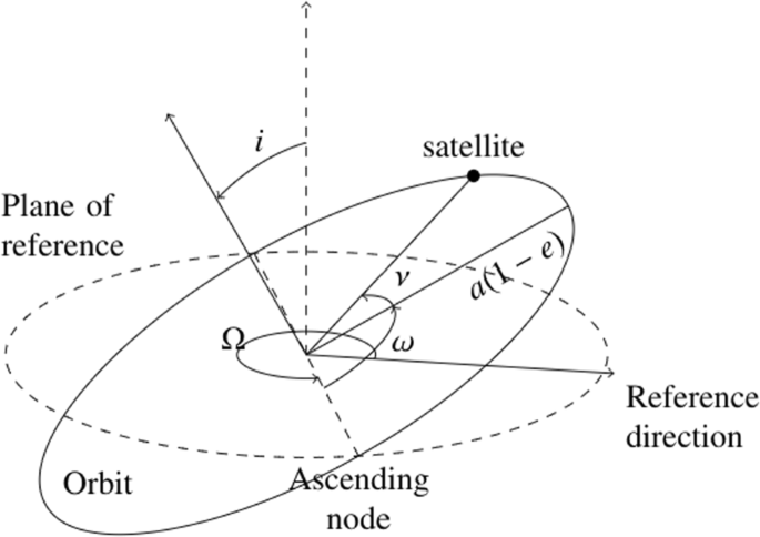

    

    Characterization of an ideal orbit and satellite position by Keplerian elements, where the reference direction is the vernal equinox direction, and the plane of reference is the Equatorial plane

  • Eccentricity (e)

• The next two parameters are describing relation between orbital plane, and the Earth’s equatorial plane, and the direction of vernal equinox:

  • Inclination (i), angle measured between the satellite orbital plane and the Earth’s equatorial plane.

  • Longitude of the ascending node (Ω), angle in Earth’s equatorial plane measured between the vernal equinox direction, and the ascending node which is the point on the satellite’s orbit where it crosses the equatorial plane, moving in the northerly direction.

• The following single parameter characterizes orientation of the ellipse in orbital plane:

  • Argument of perigee (ω), angle in the plane of the orbit, measured between the ascending node and the perigee, which is point in the satellite orbit, where the satellite is closest to the center of the Earth.

• The last Keplerian orbit parameter determines satellite position on its orbit in given time epoch:

  • True anomaly (ν), angle measured in orbital plane between perigee, and the satellite position at given time.

5.3.2 System effectiveness model almanac

Each GPS satellite distributes simple ephemerides (Keplerian orbit parameters) for whole constellation (so-called almanac). Receiving full almanac data takes 12.5 min [8]. A more practical and flexible approach is to use System Effectiveness Model (SEM) almanac available online instead of obtaining almanac transmitted by a GPS satellite. The definition of the SEM almanac content can be found in [31].

5.3.3 Satellite position computation algorithm

With the data from SEM almanac, it is possible to obtain a coarse position of all satellites in the GPS system constellation. The satellite position computation algorithm is presented below [32].

• 1. In the first step, two World Geodetic System 84 (WGS 84) constants must be introduced [32]:

  $$ \mu = 3.98605 \times 10^{14} \left[\frac{m^{3}}{s^{2}}\right], $$

  (43)

  which is WGS 84 value of the Earth’s gravitational constant for GPS users [32]. The second constant is the WGS 84 value of the Earth’s rotation rate given by

  $$ \Dot{\Omega}_{e} = 7.2921151467 \times 10^{-5} \left[\frac{rad}{s}\right] $$

  (44)

• 2. The satellite mean motion (n₀) is computed using square root of semi major axis from SEM almanac ($\sqrt {a}$):

  $$ n_{0} = \sqrt{\frac{\mu}{a^{3}}} $$

  (45)

• 3. Now, the difference between almanac time (defined by GPS Week Number - t_aw and GPS time of applicability - t_as), and the desired time (defined by weeks number - t_dw and seconds number - t_ds) is computed from the following formula:

  $$ \Delta t = t_{ds} - t_{as} + (t_{dw} - t_{aw})\cdot s, $$

  (46)

  where s is the number of seconds in a single week.

• 4. In this step, mean anomaly for desired time is obtained using mean anomaly for almanac time (M₀) from SEM almanac, and the values obtained from Eq. (45) and (46):

  $$ M = \tilde M_{0} + n_{0} \cdot \Delta t, $$

  (47)

  where $\tilde M_{0} = \pi \cdot M_{0}$, is converted to radians (1 semicircle =π radians), as SEM gives M₀ in the units of semicircles.

• 5. Eccentric anomaly (E measured in radians) can be found by solving the so-called Kepler’s equation given by

  $$ M = E - e \sin E, $$

  (48)

  where e is the eccentricity from SEM almanac. Kepler’s equation can be iteratively solved with one of the several available methods [33].

• 6. Having eccentric anomaly calculated, the GPS satellite position on the Keplerian orbit can be defined by true anomaly:

  $$ \nu = \arctan \frac{\sqrt{1-e^{2}}\sin E}{\cos E-e}, $$

  (49)

  and the radius by

  $$ r = a(1-e \cos{E}) $$

  (50)

• 7. After transformation of the satellites coordinates from radial to Cartesian, we get

  $$ \left\{\begin{array}{cc} x = r \cos{(\nu+\omega)} \\ y = r \sin{(\nu + \omega)} \end{array}\right. $$

  (51)

• 8. Next, the satellite coordinates in Keplerian orbit plane are transformed to ECEF (see Appendix A) coordinates. Two parameters are obtained to perform this operation. First, the inclination is given by

  $$ i = \tilde i_{0} + \delta \tilde i, $$

  (52)

  where both i₀ and δi are given in the SEM almanac in semicircles units and must be converted to radians ($\tilde i_{0} = \pi \cdot i_{0}$, and $\tilde \delta i = \pi \cdot \delta i$). Next, the longitude of the ascending node is

  $$ \Omega_{p} = \tilde \Omega_{0} + (\tilde{\Dot{\Omega}} - \Dot{\Omega}_{e})\Delta t - \Dot{\Omega}_{e} t_{as}, $$

  (53)

  where $\tilde \Omega _{0}= \pi \cdot \Omega _{0}$ and $\tilde {\Dot \Omega }= \pi \cdot \Dot \Omega$, because Ω₀ and $\Dot {\Omega }$ are given in SEM almanac in the units of semicircles, and semicircles/second, which are converted to the units of radians and radians/second, respectively.

• 9. The final step is to obtain the GPS satellite position in ECEF coordinates with the following formulas:

  $$ \left\{\begin{array}{ccc} x_{{\text{ECEF}}} = x \cos{\Omega_{p}} - y \cos{i} \sin{\Omega_{p}} \\ y_{{\text{ECEF}}} = x \sin{\Omega_{p}} + y \cos{i} \cos{\Omega_{p}} \\ z_{{\text{ECEF}}} = y \sin{i} \\ \end{array}\right. $$

  (54)

5.3.4 Algorithm implementation and validation

The presented GPS satellite position estimation algorithm had been implemented in Python programming language. To validate the implemented algorithm, visible satellite list had been captured from USB-GPS antenna. USB antenna outputs the data via serial port using National Marine Electronics Association (NMEA) protocol. To this end, a C++ program has been developed to capture only data frames containing information about visible satellites and log them to text file (see Fig. 7). Satellite coordinates are the azimuth (az) and the elevation (el) angles seen from GPS antenna position (52.3921476900N, 16.7982299300E). Observations were performed in a 24 h period between 29 and 30 of December 2018.

Fig. 7

Example set of the visible satellites coordinates (1^∘ resolution) extracted from NMEA data captured by G-Mouse USB antenna and logged into text file

Results of the comparison between the computed and the captured satellites coordinates are presented in Fig. 8. The former are derived by using the algorithm described in Section 5.3.3, with SEM almanac obtained 28 December 2018 19:56:48 UTC, while the latter are extracted from NMEA messages. There are two sources of errors: the first source of error is related to the 1^∘ quantization of NMEA data (even though internally GPS receivers use much more accurate satellites positioning), while satellite coordinates computed with SEM almanac data domain is continuous. Up to 0.5^∘ of error can be expected. The second source of errors is related to the computing satellites coordinates, i.e., the utilized satellites position forecasting, on the basis of ideal elliptic orbit, while in fact there are some temporary deviations in the satellites orbits.

Fig. 8

Comparison between visible satellites coordinates computed with algorithm from Section 5.3.3, and those obtained from NMEA data provided by USB antenna

As it can be observed in Fig. 8, satellites orbits prediction error doesn’t grow over the analysed time period. This turns satellite constellation obtained on the basis of the algorithm described in Section 5.3.3 to be a reasonable tool for 24 hours long simulations. Also prediction errors around 1^∘ seems to have no significant impact on the error modeling, as it is shown in Section 6.2.3.

5.4 RTK error estimation simulation environment

A block scheme illustrating initial framework for UE localization error modeling in RTK system under open-sky conditions is presented in Fig. 9. The simulation environment consists of several functional blocks presented in previous subsections: Gauss-Markov noise generators (Section 5.2.2), SEM almanac-based satellites orbit prediction (Section 5.3.3), and linear model for position estimation (Eq. (26)).

Fig. 9

Block scheme illustrating simulation environment for the RTK positioning error estimation

For a given time instance, a list of visible satellites is computed on the basis of SEM almanac with the 7^∘ elevation cutoff angle, i.e., satellites close to the horizon are treated as not visible for the UE receiver [8]. Next, on the basis of reference station position, and UE "true" position satellite-reference station, and the satellite-UE ranges are computed for each visible satellite. With the use of the independent GM process generators (with the given fix parameters: variance σ² and correlation time τ) obtained ranges are noised. Noised ranges and visible satellites coordinates are then used in linear model for position estimation to formulate Eq. (27) under the assumption of having resolved integer ambiguities. Finally the position error is computed as the difference between true UE coordinates, and the ones computed from the noised reference station-satellite and the UE-satellite ranges.

5.4.1 RTK positioning error covariance matrix estimation

In the other less computationally complex approach, the RTK positioning error covariance matrix may be estimated with the analytic formula, describing the least squares estimator covariance matrix and given by [8]

$$ {\text{cov}}(\delta \textbf x) = \left(\textbf G^{T} \textbf G\right)^{-1}\textbf G^{T} \cdot \boldsymbol{R}_{dd} \cdot \textbf G\left(\textbf G^{T} \textbf{G}\right)^{-1}, $$

(55)

where G is the satellite-reference station-UE geometry matrix (Eq. (26)), and the R_dd is the double difference correlation matrix (Eq. (16)). Unfortunately, in this approach, random variables variances, can be only obtained, with no information on the positioning error distribution. Moreover, autocorrelation function cannot be estimated.

6 Simulation results and discussion

For evaluation purposes, the environment described in Section 5.4 is implemented in python programming language. Several computer simulation experiments have been performed for various sets of input parameters. Three places globally had been chosen for simulations. These are listed in Table 1. Loc1 refers to the first author’s home near Poznan in Poland, Loc2 to the point where prime meridian intersects equator, and Loc3 to the Huawei headquarters in the Chinese city of Shenzen. The UE-reference station distance is chosen to be 130 m, 157 m, and 151 m for Loc1, Loc2, and Loc3, respectively. Choosing such distances ensures the UE and reference station are affected by the same atmospheric propagation delays, as explained in Section 5.1. This is reasonable for a dense 5G network and allows for the simplification of error modeling by assuming that errors related with ionosphere and troposphere delays are equal at UE and reference station.

Table 1 Coordinates of the reference station and UE used in the simulations

The input parameters for GM process generators, which models the UE-satellite, and reference station-satellite distance error are specified based on the measurements with the use of smartphone-grade and survey-grade GNSS antenna, respectively, under open-sky conditions done in [16]. The values of the GM process parameters are shown in Table 2. Static correlation time refers to the scenario when the receiver antenna does not move, i.e., the reference station is always static. Dynamic correlation time refers to the scenario, when UE moves randomly within the GPS L1 carrier signal wavelength. The trajectory of the receiver is modeled as a GM process and has an average speed of 7.65 $\frac {km}{h}$ [16].

Table 2 GM process parameters for modeling of undifferenced carrier phase measurement error for a static reference station

In all simulations, SEM almanac is utilized (almanac date: 28 December 2018 19:56:48 UTC). For all simulations, start date is 29 December 2018 14:58:09 UTC, and end date is 30 December 2018 14:58:09 UTC. Longer than a 24 h simulation period is not necessary due to the fact that visible satellites constellation repeats every 23 h and 56 min [8].

6.1 Continuous 24 h scenario

The first computer simulation is performed for Loc1, with static GM noise parameters. There are 15, 24-h-long simulation runs; UE position is computed in 1 s intervals. During the whole simulation experiment, the satellite constellation is continuously changing.

6.1.1 Localization error distribution

The first field of study for this simulation scenario is localization error empirical probability density function. Figure 10 present the localization error distribution in the east and north directions with fitted Gaussian functions. As can be seen, distributions have shape of the Gaussian distribution.

Fig. 10

Localization error distribution

6.1.2 Autocorrelation analysis

Apart from the localization error distribution, also the autocorrelation functions are analyzed. If the localization error can be described by GM process, autocorrelation function can be given by Eq. (28). Here, it appears the problem of fitting GM process parameters already discussed in Section 5.2.3. Correlation time is estimated with the use of (42). However, the number of the utilized autocorrelation function samples must be established. Figure 11 illustrates RMSE between the empirical autocorrelation function and fitted GM autocorrelation function while changing the number of the empirical autocorrelation function samples (N) used in the fitting process. As it can be seen, higher Nresults in lower RMSE. However, the improvement is negligible for N > 500. As such N = 500 is used in all subsequent simulation experiments.

Fig. 11

Dependence between number of utilized autocorrelation function samples used for GM process fitting and the resultant RMSE

Fig. 12

Autocorrelation of the localization error in Loc1, computed on the basis of: simulation, Eq. (42) with N = 500, and Eq. (34). σ and τ parameters are estimated with 95% confidence intervals

Autocorrelation functions for east and north directions are presented in Fig. 12. In each figure there is the autocorrelation obtained from the simulation results, and two fitted GM processes: using Eq. (42) with N = 500 and using (34). It can be seen that the fitted GM process autocorrelation function approximates the one obtained from simulation results very well. This, along with the localization error samples following the Gaussian distribution, leads to the conclusion that the UE localization error in RTK system may be modeled as a GM process.

To check if there is a correlation between RTK localization error in the east and north directions, the correlation coefficient (see [34]) has been computed with the result of − 0.0669. A correlation coefficient close to 0 leads to the conclusion that east and north localization errors are uncorrelated and can be modeled independently. With other words independent GM process generators can be utilized to produce east and north localization error.

6.2 Step 24 h scenario

All previous simulations revealed that RTK localization errors in east and north directions are uncorrelated and may be modeled as a GM process. Next, we study the influence of the visible GPS satellites geometry on the RTK localization error at a given time and geographical position.

Simulation is performed in a "step mode." Every single step is related to a constant satellites constellation, and 15 independent simulation runs, each utilizing a different random generator seeds. During each simulation run, 3600 UE position error samples are collected at 1 Hz sampling frequency. From 29 December 2018 14:58:09 UTC to 30 December 2018 14:58:09 UTC, a new satellite constellation is computed every 10 min, and the corresponding simulations are performed, resulting in 144 steps. The simulations are performed for all locations in Table 1, static reference station and static/dynamic UE.

6.2.1 Variance analysis

Firstly, RTK localization error variance obtained with the use of the simulation environment presented in Section 5.4 is compared with the one estimated using analytical formula (55), as it is depicted in Fig. 13 for Loc1. The variance obtained with (55) visibly overlap with simulation results for the dynamic UE. In the static UE scenario variance obtained on the basis of simulation and Eq. (55) differs more. This can be caused by longer correlation time (300 s) that results in smaller number of independent localization error samples over the simulated period. However, it can be stated that the estimated variance is independent of UE motion. Additionally, it is confirmed that the localization variance can be generated using (55) instead of performing full system simulations. In Fig. 14, localization error variances obtained on the basis of (55) for all considered geographical localizations are compared for the same time instances. It can be observed that the results differ significantly. This implies that RTK localization error variance depends on the visible satellites geometry.

Fig. 13

Comparison between RTK localization error variance in Loc1 obtained from simulations, and computed with Eq. (55)

Fig. 14

Comparison between RTK localization error variances obtained at different geographical localization

6.2.2 Correlation time analysis

Apart from the variance, the GM process is also described by correlation time. As an example, simulation results obtained for Loc1 are presented in Fig. 15, in the case of dynamic UE, and Fig. 16, in the case of static UE. In both presented examples, the correlation time seems to be randomly fluctuating around a mean value, with no dependence of daytime or geographical localization. This hypothesis is validated by means of analysis of variance (ANOVA) statistical test on the correlation time data. ANOVA is a statistical test that allows to check if several data sets have statistically equal means, by analysis of their variance [35]. The ANOVA test has been independently performed for each simulation scenario and for all data sets related with static and dynamic UE respectively. The aim of the ANOVA test was to reject or not hypothesis h₀ that all data sets (correlation time over daytime and geographical localization) have the same mean value. To reject or not hypothesis, the ANOVA test output, i.e., p value, is compared with the so-called significance level (α), i.e., the probability of rejecting hypothesis which is actually true (typical α value is 0.05) [35]. The hypothesis may be rejected with significance level α when pvalue <α. The corresponding ANOVA results are presented in Table 3. The hypothesis is rejected only in the case with dynmic UE in east direction and Loc2.

Fig. 15

Correlation time obtained on the basis of simulation results in Loc1 and for the dynamic UE

Fig. 16

Correlation time obtained on the basis of simulation results in Loc1,and for the static UE

Table 3 ANOVA statistical tests results for localization error correlation times

In conclusion, the RTK localization error correlation time depends only on undifferenced carrier phase measurement error and is independent of daytime and geographical localization, i.e., visible satellites constellation. The mean values of correlation time, averaged over all 144 steps, for all of studied geographical locations are presented in Table 4. For dynamic UE localization error correlation time in both east and north directions can be assumed to be 2 s. The mean value of the correlation times in the case of static UE (in both east and north directions) is 255.2 s and fits in the confidence intervals in Table 4.

Table 4 RTK east and north localization error correlation times, averaged over 24 h with 95% confidence intervals

6.2.3 Visible satellites coordinates resolution analysis

The proposed RTK localization error framework rely on visible satellites coordinates. The utilized satellites localization prediction uses SEM almanac introducing typically 1–2 km error (as mentioned in Section 5.3). The aim of this section is to verify whether degradation of satellites coordinates accuracy significantly impacts the final UE localization error. On the basis of Eq. (55), the localization error variance for Loc1 geographical localization is computed with the visible satellites coordinates rounded to 1^∘ and compared with the full-accuracy results in Fig. 17. As it can be seen, the presented results are almost identical.

Fig. 17

RTK localization error variance, computed with Eq. (55), for non-rounded and rounded to 1^∘ satellites coordinates (az,el) in Loc1

6.2.4 Adaptation of the proposed scheme for urban environment

In addition, the proposed RTK localization error framework may be applied to provide initial estimate of the localization error in urban environment, i.e., without taking into account NLoS UE-satellite signals propagation or cycle-slip occurrence. This can be done by increasing the elevation cutoff angle α_el from the default 7^∘ to the value related to street geometry: width W and neighboring buildings height H as depicted in Fig. 18. This approach mimics signals from some GNSS satellites being blocked by buildings.

Fig. 18

RTK LoS under urban conditions, modeled by adjusting elevation cutoff angle α_al to the street geometry: width W and height H

Dependence between street geometry of width W, and height H, and elevation angle cutoff α_el is given by

$$ \alpha_{el} = \arctan{\left(\frac{2H}{W}\right)}. $$

(56)

A simulation was performed to estimate RTK localization error variance in Loc1 while changing α_el. The elevation angle was increased to the value of 18^∘ that corresponds to the $\frac {H}{W}$ street geometry ratio equal to 0.162. Results are depicted in Fig. 19. As expected, a higher elevation cutoff angle causes fewer satellites visibility. This finally results in a larger localization error in relation to the one obtained with default 7^∘ elevation cutoff angle.

Fig. 19

RTK localization error variance obtained at Loc1 for open-sky and urban scenario modeled with elevation cutoff angles 7^∘ and 18^∘, respectively

7 Final RTK localization error modeling algorithm

On the basis of the previous results a RTK localization error model for smartphone-grade GNSS antenna under open-sky conditions is proposed. Simulation experiments from Section 6.1 shown that RTK localization errors in both east and north directions are uncorrelated and may be modeled as a GM process. Further simulations from Section 6.2 proved that there is a dependence between localization error variance and geographical localization and daytime as a result of the different visible satellites geometry. The localization error correlation time seems to be related to the UE motion. The proposed model considers correlation time for two scenarios. First, it is appropriate for static UEs, e.g., people sitting on the bench in a park. Second, it can be applied for dynamic UEs, e.g., fast walking pedestrians. However, additional studies would be required to obtain a mathematical formula to express the dependence of UE speed and RTK error correlation time, necessary for dealing with a big amount of other cases.

Figure 20 illustrates a block diagram representing the proposed RTK localization error generator. There are two independent GM process generators (see Section 5.2.2), one for error generation in the east direction and another one for the error generation in north direction, as the east and north localization errors are assumed to be uncorrelated. Furthermore, the GM process is described by two parameters: correlation time τ and variance σ², and can be generated as depicted in Fig. 21. Equation (32) explains how to convert given GM process parameters: correlation time and variance, into the generator parameters (a₁ and $\sigma ^{2}_{s}$ from Fig. 21).

Fig. 20

Block diagram of the RTK localization error generator

Fig. 21

GM process generator structure

Simulation results show that localization error correlation time depends only on the UE motion. For static UEs, it is assumed to be the 255.2 s, while for dynamic UEs (moving with average speed of 7.65 $\frac {km}{h}$), it is assumed to be 2 s.

The variances of east and north localization errors change over geographical localization and daytime. Therefore, variance in both east and north directions will be computed with Eq. (55) using geometry matrix (see Eqs. (26, 25)). First, the GPS satellites coordinates (for every satellite in the constellation) are obtained on the basis of SEM almanac (see Section 5.3.2), with the use of the algorithm described in Section 5.3.3. Then visible satellites are those for which elevation angle (measured from the reference station) is greater than 7^∘.

Finally, undifferenced error standard deviation values obtained on the basis of experimental measurements in [16] and related to the UE (σ_u=2.5 mm) and reference station (σ_r=6 mm), required in the Eq. (55) are taken from Table 2.

Additionally, RTK localization error under urban conditions can be initially modeled by adjusting the elevation cutoff angle to the street geometry as proposed in Section 6.2.4.

8 Conclusions

The UE localization in 5G networks will be used not only for commercial and emergency purposes, but also for network optimization, intelligent transportation systems, and industrial applications. One of the most promising localization methods already described in LPP and foreseen for NR is GNSS-based RTK method providing centimeter-level accuracy.

The aim of this paper is to study daytime, geographical localization, and UE motion impact on the resulting RTK localization error and its distribution under open-sky conditions. For evaluation purposes a simulation environment is proposed and implemented including implementation and validation of the GM process generators, implementation of the satellite position computation algorithm (on the basis of the SEM almanac), and implementation of the program capturing real visible satellite data (with the use of the NMEA protocol).

A series of simulations have been performed to study the impact of geographical position, daytime, and UE motion on the RTK localization error variance and correlation time. As a conclusion, the RTK localization error may be modeled with a Gauss-Markov process, described by time-varying variance, dependent on UE geographical position and daytime, and constant correlation time dependent on UE motion.

Finally, on the basis of the simulation results, the RTK localization error model has been proposed. It could be a useful tool for simulations studying performance of the future 5G networks utilizing REMs or intelligent transportation systems.

Future work include the study of imperfections in the UE-reference station side link quality and their impact on the RTK localization error.

9 Appendix A: Coordinates Systems

In this paper, various global coordinates systems (e.g., Earth-Centered Earth-Fixed, east-north-up) are mentioned in several places. The purpose of this appendix is to describe them, and introduce transformations between them.

All coordinates systems described here refer to the World Geodetic System 1984 (WGS 84), which is currently the official geodetic system for navigation, mapping and charting purposes [8]. WGS 84 defines the Earth-Centered Earth-Fixed (ECEF) cartesian coordinate frame, geometric model of Earth’s shape, the Earth’s gravity field, and a set of constants (e.g., Earth’s gravitational constant, Earth’s rotation rate, used in Section 5 during GPS satellites orbits computation process) [8].

9.1 Geodetic

Geodetic coordinate system (Fig. 22) characterizes point near Earth’s surface with the following set of coordinates [36]:

• longitude λ in the range of (− 180^∘ to 180^∘) measured between Prime Meridian and desired point

  Fig. 22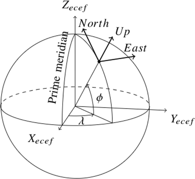

  

  Comparison of Earth-Centered Earth-Fixed (ECEF), East-North-Up (ENU) and geodetic coordinate systems

• latitude ϕ - in the range of (− 90^∘ to 90^∘) measured between the equatorial plane and the normal of the reference ellipsoid that passes through the measured point

• The height h (or altitude) is the local vertical distance between the measured point and the reference ellipsoid surface

9.2 Earth-centered Earth-fixed

ECEF coordinate system (Fig. 22) is an inertail coordinates system (rotates with Earth). In result, any chosen fixed point on the Earth surface has fixed set of coordinates. The origin of ECEF coordinate system is located in the center of Earth, and the axes are defined in following form: [36]

• Z-axis is along the spin axis of the Earth, pointing to the north pole

• X-axis intersects the sphere of the Earth at 0^∘ latitude and 0^∘ longitude

• Y-axis is orthogonal to the Z- and X-axes with the usual right-hand rule

9.3 East-north-up

East-north-up (ENU) coordinate system (Fig. 22) is so-called local-level-system. Its origin is defined at the given position (e.g., reference station position), axis are defined in following form [8]:

• Axis-1 points east

• Axis-2 points north

• Axis-3 points upward

9.4 Coordinates transformations

Coordinates systems transformations that are necessary for computer simulations of the RTK localization error will be described here. For details please refer to [36], [8].

9.4.1 Geodetic-ECEF

To perform transformation between geodetic coordinates (λ,ϕ,h) to ECEF (x, y, z) two parameters from WGS 84 describing Earth’s Meridian ellipse (defined as connection between all points on the ellipsoid with λ=const [8]) must be introduced [36]:

$$ \left\{\begin{array}{ccc} a_{wgs} = 6378137m \\ e_{wgs} = 0.08181919, \end{array}\right. $$

(57)

where a_wgs is the semi major axis and e_wgs is the eccentricity of the meridian ellipse.

Let’s define now constant N to simplify calculations [36]:

$$ N = \frac{a_{wgs}}{\sqrt{1 - e_{wgs}^{2} sin^{2} \phi}}. $$

(58)

Geodetic to ECEF transformation is given with the following formula [36]:

$$ \left[\begin{array}{cccc} x \\ y \\ z \end{array}\right] = \left[\begin{array}{cccc} (N + h) \cdot \cos{\phi} \cos{\lambda} \\ (N + h) \cdot \cos{\phi} \sin{\lambda} \\ (N(1-e_{wgs}^{2}) + h) \cdot \sin{\phi} \end{array}\right] $$

(59)

Inverse coordinates transformation is more complex and will not be discussed, because it is not necessary for the implementation of simulation environment.

9.4.2 ECEF-ENU

As mentioned before, ENU is a local-level-system, performing transformation of the point in ECEF system (e.g., satellite coordinates x_s=(x_s,y_s,z_s)^T), reference point (e.g. reference station) coordinates in ECEF (x₀=(x₀,y₀,z₀)^T), and Geodetic (λ₀,ϕ₀,h₀)) systems are necessary.

The main part of the transformation is the rotation matrix R_enu. This matrix rotates ECEF axes to make them coincident with the ENU axes. R_enu is given as [8]:

$$ \textbf R_{{\textrm{enu}}} = \begin{bmatrix} -\sin{\lambda_{0}} & \cos{\lambda_{0}} & 0 \\ -\sin{\phi_{0}}\cos{\lambda_{0}} & -\sin{\phi_{0}}\sin{\lambda_{0}} & \cos{\phi_{0}} \\ -\cos{\phi_{0}}\cos{\lambda_{0}} & -\cos{\phi_{0}}\sin{\lambda_{0}} & \sin{\phi_{0}} \end{bmatrix}. $$

(60)

Now x_s in ENU coordinates ($\textbf x_{s_{{\textrm {enu}}}} = (e_{s}, n_{s}, u_{s})^{T}$) is given with the following formula [8]:

$$ \textbf x_{s_{{\textrm{enu}}}} = \textbf R_{{\textrm{enu}}}(\textbf x_{s} - \textbf x_{0}) $$

(61)

Sometimes it is more useful to express position in ENU system with the azimuth (az) and elevation (el) angles (e.g., satellite position with respect to the reference station). Azimuth angle (0^∘−360^∘) is measured clockwise from the north, and elevation angle (0^∘−90^∘) is measured from local horizon (positive up coordinate). ENU can be transformed to az and el with the following formulas [8]:

$$ \tan{az} = \frac{e_{s}}{n_{s}} $$

(62)

$$ \sin{el} = \frac{u_{s}}{\sqrt{e_{s}^{2} + n_{s}^{2} + u_{s}^{2}}} $$

(63)

References

J. A. del Peral-Rosado, R. Raulefs, J. A. López-Salcedo, G. Seco-Granados, Survey of cellular mobile radio localization methods: From 1g to 5g. IEEE Commun. Surveys Tutor.20(2), 1124–1148 (2018). https://doi.org/10.1109/COMST.2017.2785181.
IRACON COST Action CA15104, T. Pedersen, B. Fleury, Whitepaper on New Localization Methods for 5G Wireless Systems and the Internet-of-Things. COST Action CA15104, IRACON (2018). https://vbn.aau.dk/en/publications/whitepaper-on-new-localization-methods-for-5gwireless-systems-an.
A. Prasad, M. A. Uusitalo, Z. Li, P. Lunden, in 2016 IEEE Globecom Workshops (GC Wkshps). Reflection environment maps for enhanced reliability in 5g self-organizing networks, (2016), pp. 1–6. https://doi.org/10.1109/GLOCOMW.2016.7849019.
A. Kliks, B. Musznicki, K. Kowalik, P. Kryszkiewicz, Perspectives for resource sharing in 5g networks. Telecommun. Syst.68(4), 605–619 (2018). https://doi.org/10.1007/s11235-017-0411-3.
H. B. Yilmaz, T. Tugcu, F. Alagöz, S. Bayhan, Radio environment map as enabler for practical cognitive radio networks. IEEE Commun. Magazine. 51:, 162–169 (2013).
3GPP, Evolved Universal Terrestrial Radio Access Network (E-UTRAN); Stage 2 functional specification of User Equipment (UE) positioning in E-UTRAN.Tech. Specification (TS) 36.305. https://portal.3gpp.org/desktopmodules/Specifications/SpecificationDetails.aspx?specificationId=2433.
D. Dardari, A. Conti, U. Ferner, A. Giorgetti, M. Z. Win, Ranging with ultrawide bandwidth signals in multipath environments. Proc. IEEE. 97(2), 404–426 (2009). https://doi.org/10.1109/JPROC.2008.2008846.
P. Misra, P. Enge, Global Positioning System: Signals, Measurements, and Performance (Ganga-Jamuna Press, 2006). https://books.google.pl/books?id=pv5MAQAAIAAJ. Accessed 24 Jul 2019.
F. Wen, H. Wymeersch, B. Peng, W. P. Tay, H. C. So, D. Yang, A survey on 5g massive mimo localization. Digital Signal Process. (2019). https://doi.org/10.1016/j.dsp.2019.05.005.
Q. D. Vo, P. De, A survey of fingerprint-based outdoor localization. IEEE Commun. Surveys Tutor.18(1), 491–506 (2016). https://doi.org/10.1109/COMST.2015.2448632.
M. Hoffmann, H. Bogucka, in Cognitive Radio-Oriented Wireless Networks, ed. by A. Kliks, P. Kryszkiewicz, F Bader, D. Triantafyllopoulou, C. E. Caicedo, A. Sezgin, N. Dimitriou, and M. Sybis. Localization techniques for 5g radio environment maps (Springer International PublishingCham, 2019), pp. 232–246.
P. Ranacher, R. Brunauer, W. Trutschnig, S. Van der Spek, S. Reich, Why gps makes distances bigger than they are. Int. J. Geogr. Inf. Sci.30(2), 316–333 (2016). https://doi.org/10.1080/13658816.2015.1086924.
3GPP, Radio Frequency (RF) pattern matching location method in LTE. Tech. Rep. (TR) 36.809. https://portal.3gpp.org/desktopmodules/Specifications/SpecificationDetails.aspx?specificationId=2488.
J. Turkka, T. Hiltunen, R. U. Mondal, T. Ristaniemi, in 2015 International Symposium on Wireless Communication Systems (ISWCS). Performance evaluation of lte radio fingerprinting using field measurements, (2015), pp. 466–470. https://doi.org/10.1109/ISWCS.2015.7454387.
3GPP, Technical Specification Group Radio Access Network; Study on NR positioning support. Technical Report (TR) 36.305, 3rd Generation Partnership Project (3GPP) (March 2019). Version 2.1.0.
K. M. Pesyna, Advanced techniques for centimeter-accurate gnss positioning on low-cost mobile platforms. PhD thesis, (2015). https://repositories.lib.utexas.edu/handle/2152/33256?show=full.
M. Fortunato, J. Critchley-Marrows, M. Siutkowska, M. L. Ivanovici, E. Benedetti, W. Roberts, in 2019 European Navigation Conference (ENC). Enabling high accuracy dynamic applications in urban environments using ppp and rtk on android multi-frequency and multi-gnss smartphones, (2019), pp. 1–9. https://doi.org/10.1109/EURONAV.2019.8714140.
J. Miguez, J. Gisbert, J. A. Garcia-Molina, P. Zoccarato, P. Crosta, L. Ries, R. Perez, G. Seco-Granados, C. Massimo. Multi-gnss dynamic high precision positioning in urban environment, (2017), pp. 408–416. https://doi.org/10.33012/2017.15197.
R. Emardson, P. Jarlemark, J. Johansson, S. Bergstrand, M. Lidberg, B. Jonsson, Measurement accuracy in network-rtk. Bollettino Geod. Sci. Affini (2009).
J. Chung, An accuracy study of rtk gnss positioning applied to comparing maps for bentgrass habitat modeling. PhD thesis (2017). Doctoral Dissertations. 1604. https://opencommons.uconn.edu/dissertations/1604.
J. Hwang, H. Yun, Y. Suh, J. Cho, D. -H. Lee, Development of an rtk-gps positioning application with an improved position error model for smartphones. Sensors (Basel, Switzerland). 12:, 12988–3001 (2012). https://doi.org/10.3390/s121012988.
M. Pesko, T. Javornik, A. Kosir, M. Štular, M. Mohorcic, Radio environment maps: The survey of construction methods. KSII Trans. Internet Inf. Syst.8: (2014). https://doi.org/10.3837/tiis.2014.11.008.
J. Perez-Romero, A. Zalonis, L. Boukhatem, A. Kliks, K. Koutlia, N. Dimitriou, R. Kurda, On the use of radio environment maps for interference management in heterogeneous networks. IEEE Commun. Magazine. 53(8), 184–191 (2015). https://doi.org/10.1109/MCOM.2015.7180526.
R. Di Taranto, S. Muppirisetty, R. Raulefs, D. Slock, T. Svensson, H. Wymeersch, Location-aware communications for 5g networks: How location information can improve scalability, latency, and robustness of 5g. IEEE Signal Process. Magazine. 31(6), 102–112 (2014). https://doi.org/10.1109/MSP.2014.2332611.
D. Slock, in 2012 5th International Symposium on Communications, Control and Signal Processing. Location aided wireless communications, (2012), pp. 1–6. https://doi.org/10.1109/ISCCSP.2012.6217868.
N. Wen, R. Berry, in 2006 40th Annual Conference on Information Sciences and Systems. Information propagation for location-based mac protocols in vehicular networks, (2006), pp. 1242–1247. https://doi.org/10.1109/CISS.2006.286655.
K. M. Pesyna, T. E. Humphreys, R. W. Heath, T. D. Novlan, J. C. Zhang, Exploiting antenna motion for faster initialization of centimeter-accurate gnss positioning with low-cost antennas. IEEE Trans. Aerospace Electron. Syst.53(4), 1597–1613 (2017). https://doi.org/10.1109/TAES.2017.2665221.
P. Lamon, The Gauss–Markov Process (Springer, Berlin, Heidelberg, 2008). https://doi.org/10.1007/978-3-540-78287-2_9. https://doi.org/10.1007/978-3-540-78287-2_9.
J. G. Proakis, D. G. Manolakis, Digital Signal Processing - Principles, Algorithms and Applications (2. Ed.) (Macmillan, 1992).
M. J. M. Y. Jun Wang, in Proceedings of the 24th International Technical Meeting of the Satellite Division of The Institute of Navigation (ION GNSS 2011). Predicting glonass satellite orbit based on an almanac conversion algorithm for controlled ionosphere scintillation experiment planning, (2011), pp. 3118–3124.
S. C. 300N. SepulvedaBlvd. SAICGPSSE&I, Navstar gps control segment to user support community interfaces. Technical Report (TR) ICD-GPS-870. https://www.gps.gov/technical/icwg/ICD-GPS-870A.pdf. Accessed 03 Aug 2019.
S. Applications International Corporation, Interface Specification IS-GPS-200 Revision E. Navstar GPS Space Segment/Navigation User Interfaces (Space and Missile Systems Center (SMC) Navstar GPS Joint Program Office (SMC/GP), 2010). https://www.gps.gov/technical/icwg/IS-GPS-200J.pdf.
M. Murison, A Practical Method for Solving the Kepler Equation (U.S. Naval Observatory, 2006). https://doi.org/10.13140/2.1.5019.6808.
B. Madsen, Statistics for Non-Statisticians (Springer, 2011). https://books.google.pl/books?id=JrC7DAEACAAJ. Accessed 19 Aug 2019.
M. Reichenbächer, J. W. Einax, Statistical Tests (Springer, Berlin, Heidelberg, 2011). https://doi.org/10.1007/978-3-642-16595-5_3. https://doi.org/10.1007/978-3-642-16595-5_3.
G. Cai, B. Chen, T. Heng Lee, Unmanned Rotorcraft Systems (Springer, 2011). https://doi.org/10.1007/978-0-85729-635-1.
Acknowledgements
Not applicable.
Funding
This work was supported by Huawei Technologies within project ’RSM Based Radio Resource Provisioning for Spectral-, Energy- and Computational Efficiency in 5G Networks’. Project no. 08/81/PRJG/8139.
Author information
Authors and Affiliations
Contributions
MH was responsible for literature study, proposal of the error generating algorithm, generation of results, and initial text preparation. PK and GK were responsible for discussing the material, shaping the manuscript, and writing/reviewing text. All authors read and approved the final manuscript.
Corresponding author
Ethics declarations
Competing interests
The authors declare that they have no competing interests.
Additional information
Publisher’s Note
Springer Nature remains neutral with regard to jurisdictional claims in published maps and institutional affiliations.
Rights and permissions
Open Access This article is distributed under the terms of the Creative Commons Attribution 4.0 International License (http://creativecommons.org/licenses/by/4.0/), which permits unrestricted use, distribution, and reproduction in any medium, provided you give appropriate credit to the original author(s) and the source, provide a link to the Creative Commons license, and indicate if changes were made.
About this article
Cite this article
Hoffmann, M., Kryszkiewicz, P. & Koudouridis, G.P. Modeling of Real Time Kinematics localization error for use in 5G networks. J Wireless Com Network 2020, 31 (2020). https://doi.org/10.1186/s13638-020-1641-8
Received:
Accepted:
Published:
DOI: https://doi.org/10.1186/s13638-020-1641-8