- Research
- Open access
- Published:
High precision hybrid RF and ultrasonic chirp-based ranging for low-power IoT nodes
EURASIP Journal on Wireless Communications and Networking volume 2020, Article number: 187 (2020)
Abstract
Hybrid acoustic-RF systems offer excellent ranging accuracy, yet they typically come at a power consumption that is too high to meet the energy constraints of mobile IoT nodes. We combine pulse compression and synchronized wake-ups to achieve a ranging solution that limits the active time of the nodes to 1 ms. Hence, an ultra low-power consumption of 9.015 µW for a single measurement is achieved. The operation time is estimated on 8.5 years on a CR2032 coin cell battery at a 1 Hz update rate, which is over 250 times larger than state-of-the-art RF-based positioning systems. Measurements based on a proof-of-concept hardware platform show median distance error values below 10 cm. Both simulations and measurements demonstrate that the accuracy is reduced at low signal-to-noise ratios and when reflections occur. We introduce three methods that enhance the distance measurements at a low extra processing power cost. Hence, we validate in realistic environments that the centimeter accuracy can be obtained within the energy budget of mobile devices and IoT nodes. The proposed hybrid signal ranging system can be extended to perform accurate, low-power indoor positioning.
1 Introduction
Accurate positioning of users and devices plays a major role in the growing number of location-aware applications. In time-based localization ranging systems, acoustic signals are inherently interesting candidates for precise ranging thanks to their relatively low propagation speed. They do not require high processing speeds, nor the same level of synchronization accuracy as RF-based systems. However, they are receptive to environmental and room characteristics, such as temperature, relative air velocity, reflection, and diffraction, impacting the accuracy of the measurements [1]. Hybrid signal ranging [2, 3] combines the advantages of both wave types: an RF signal is used as timing reference and the time difference with the slower propagating (ultra)sound signal is used to calculate the distance. Two classes of hybrid RF/acoustic techniques have been proposed: indirect and self positioning. An example of the first is the Active Bat Local Positioning System [4]. The base stations are attached to the ceiling and periodically broadcast a radio message containing a single identifier, causing the corresponding mobile node to emit a short encoded ultrasound pulse. The position is then calculated at a central point using the time of arrival (ToA) at the different beacons. The second technique is used by the Cricket System [5]. Here, the base stations simultaneously emit ultrasonic and radio pulses for time difference of arrival (TDoA) calculations. The mobile device calculates its own position, which ensures its privacy. Several hybrid signaling studies have focused on obtaining high accuracy with as little infrastructure as possible [6, 7], paying little or no attention to the energy constraints of mobile devices. To address this, short-range, backscattering-based approaches have been proposed with high precision but complex system architecture [8, 9].
We present three main contributions in this paper. The first is a novel hybrid RF-acoustic signaling that performs a just-in-time wake-up of the nodes. This concept enables ultra low power consumption at the mobile node. Secondly, we propose fast and lightweight algorithmic solutions to resolve incorrect measurements due to reflective acoustic signals. The third contribution is the realization of an experimental set-up that was used to validate the results in real-life proof of concept.
The presented technology enables ultra low power localization in several industrial and healthcare applications like wayfinding and contact tracing in large venues, real-time customer behavior analysis in retail, indoor positioning in large warehouses and production sites, and wander detection and localization of residents in assisted living facilities.
This paper is further organized as follows. The next section introduces the chirp-based ranging concept, focusing on high accuracy and ultra-low power consumption. In Section 3, the proposed system’s accuracy is assessed, based on three indoor environments with different room characteristics. Section 4 compares three low complexity solutions to enhance the accuracy. We present our experimental setup, hardware design and measurement results in Section 5. The last section of this paper summarizes the conclusions and discusses the potential future work.
2 Methods
2.1 Ultra low-power hybrid acoustic-RF ranging concept
A straightforward approach for hybrid RF/acoustic ranging—also used in the Cricket system [5]—is to simultaneously transmit the signals. Hence, at the receiver side, the RF signal arrives quasi-instantaneous and serves as a time reference. Consequently, the propagation delay of the acoustic signal is measured to calculate the distance between transmitter and receiver. While this method offers high precision, it is not well suited for low-power devices as both sides of the link require significant energy:
-
The transmitter needs to power a loudspeaker, which is approximately 150 times more power hungry than transmitting RF [10, 11]. Hence, the Active Bat topology [4], where the mobile nodes emit ultrasonic signals, is not appropriate for energy constrained nodes.
-
The receiver needs to stay powered on for a relatively long time waiting for the acoustic signal to arrive, e.g., 30 ms for an operation area with a radius of about 10 m.
We propose an alternative solution that addresses the above challenges by:
-
1.
First, starting the transmission of an acoustic signal only by a powered beacon. Shifting the higher power demanding audio transmission to the beacon enables the desired low power mobile nodes. The signal has a predetermined duration and it is modulated in order to enable the extraction of delay information later on. The system presented in this paper uses a chirp signal.
-
2.
Second, transmitting the RF signal at the end of the transmission of the acoustic signal, to wake up all receivers simultaneously for a short duration only.
Note that acoustic wake-up sensors [12, 13] can also be considered to avoid a long “on-time” of nodes waiting for the signal to arrive. However, these typically generate frequent false wake-ups caused by ambient sounds, decreasing the energy efficiency and system accuracy drastically. Another convenient strategy could be to broadcast audio at fixed time intervals. In these scenarios, clock drift should be countered by performing timing synchronization between the transmitting and receiving side, leading to a more complicated and power hungry system architecture. Our proposed system can transmit the hybrid signals at its own convenience and is clock drift independent thanks to the RF-signals both acting as a time reference and communication backbone. Advantages of this system are the reduction of the awake times to milliseconds, the prevention of false wake-ups and the opportunity to use ultrasonic sound signals, enabling human unaware, acoustic positioning, and easy synchronization with RF.
2.2 Hybrid RF-ultrasonic system
The proposed hybrid RF/ultrasonic ranging system concept is shown in Fig. 1. A list of the used notations can be found in Table 1. In its generic form, it consists of a single beacon (B) and one or more mobile nodes (Mx). The beacon is able to wake up all the mobile nodes simultaneously by a single RF signal (mRF(t)). A distance measurement is performed as follows:
-
1.
The beacon starts broadcasting an audio signal (ma(t)) with a certain duration (τtx) at starting time (T0).
Fig. 1 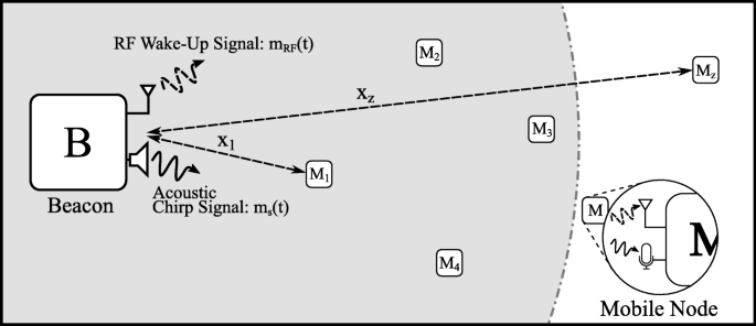
Ranging system setup. The beacon periodically transmits a sound signal. All ultra low-power nodes are woken up and synchronized on basis of the RF signal
Table 1 Table of notations -
2.
At a given time (TA≥T0), all mobile nodes wake up simultaneously for a short time (τrx) and receive, depending on their distance to the beacon, a specific part of the delayed, distorted audio broadcast.
-
3.
Pulse compression is performed on the smaller, received audio snippet resulting in a distance estimation.

Figure 2 shows a timing diagram for an exemplary case with three mobile nodes. This timing overview illustrates the difference between the proposed concept and conventional hybrid RF/acoustic TDoA systems. All mobile nodes wake up at the same time, and the ranging information is comprised in the received audio signals (Δfrx,1 for M1, Δfrx,2 for M2) at the wake-up time of the mobile nodes (TA in all cases). The restricted awake time reduces the power consumption. However, it impacts the accuracy of the measurements, which is limited by the duration of the reception window τrx and the perceived frequency swing of Δftx.

Timing overview of the transmitter and three mobile nodes as in the setup in fig. 1. Mobile nodes 1 and 2 are within the range of the beacon, mobile node z is not. The distances to the transmitter are calculated based on the received sound chirp
The ranging coverage of the systemFootnote 1 is determined by the audio broadcast duration at the transmit side (τtx) and the speed of sound. For example, for a sound signal with a duration of 30 ms and a speed of sound of vs = 340 m/s, the coverage is limited to 10.2 m. Figure 3 illustrates the three possible ranging scenarios.

Three ranging scenarios at different RF wake-up signal times
The first scenario depicts the standard operation. Here, the receivers should wake up as late as possible. More specific, the RF wake-up signal is sent at the very end of the acoustic signal, i.e., TA=(T0+τtx)−τrx. Mz (see Figs. 1 and 2) is too far away from the beacon to receive the sound signal when it wakes up, since \((\frac {x_{z}}{v_{s}} > T_{A}-T_{0})\). It is therefore incapable of calculating its distance to the beacon.
The second scenario illustrates what happens when the RF wake-up signal is sent earlier during the audio broadcast. This reduces the maximum ranging coverage.
A last scenario shows what happens if the RF-awake signal is sent after the audio broadcast. Here, the receivers close to the beacon are incapable of calculating their distance as they do not receive a direct audio signal during their wake-up period. On the contrary, the maximum distance to the beacon is increased.
The sampled audio in the awake state can be used for local processing (self positioning) or can be transmitted to a central unit (indirect positioning). Two-dimensional positioning of the mobile node can be achieved by adding at least two more beacons to the system in Fig. 1. The acquired, relative distances to these beacons can be used in multilateration or other geometric models to find the position of the mobile nodes [14]. Identification of the sound signal is crucial here, and multiple access techniques (e.g., FDMA, TDMA, CDMA) as proposed by [15–17] can achieve this. These scheme are outside the scope of this paper which focuses on the proposed ranging system in reverberant and noisy environments.
2.3 Pulse compression
Autocorrelation is used to perform fast distance calculations using small data sets, as described in [18, 42], and exploited in [19, 20]. A linear chirp [21–23] is used as audio broadcast signal for two reasons. First of all, mobile nodes with different distances to the beacon, will measure other parts of the chirp signal. They can rely solely on the measured frequency shift Δftx to compute their distance to the beacon. Secondly, when processing, chirps have compressed inter-correlation signals [24].
A linear chirp, sc(t), can be described as:
where τrx is the pulse duration, A the amplitude of a rectangle window function, f0 is the carrier frequency, and Δftx is the nominal chirp bandwidth. The equation for the instantaneous frequency f(t) shows this linear ramp of the chirp:
where ϕ(t) is the phase of the chirped signal.
Cross correlation/autocorrelation of linear chirps results in a form of pulse compression. Cross correlation between the transmitted and received signal can be achieved by convolution of the received signal with the conjugated and time-reversed transmitted signal:
It can be shown [25] that the autocorrelation of a chirp signal is given by:
with Λ a triangle function, with a value of 0 on \([\text {-}\infty, \text {-}\frac {1}{2}]\cup [\frac {1}{2},\infty ]\) and linearly increasing on \([\frac {-1}{2},0]\) where it has its maximum 1, and then decreasing linearly on \([0,\frac {1}{2}]\). Around the maximum, this function behaves like a cardinal sine, with a -3 dB width of \(\tau ' \approx \frac {1}{\Delta f_{rx}}\). For common values of Δfrx, τ′ is smaller than τrx, hence the name pulse compression.
The pulse compression ratio can be described as the ratio between the received pulse and the compressed pulse duration:
This equation can be rewritten as the time bandwidth product, which is generally larger than 1. As the energy of the signal is kept constant when pulse compression is performed, the energy gets concentrated in the main lobe of the cardinal sine, resulting in an SNR-gain proportional to the compression ratio.
There are three parameters in Eq. (5) that can increase the SNR-gain and inherently result in more accurate distance calculations.
-
1.
The nominal chirp bandwidth (Δftx), limited by the frequency response of the ultrasonic microphone or speaker. Typically for low cost, low-power mobile acoustic nodes, MEMS microphones are used, e.g., Knowles SPU1410LR5H [26]. Figure 4a shows the frequency and noise response of this MEMS microphones. A theoretical − 3 dB bandwidth of 75 kHz is depicted in this picture. Empirical measurement with the microphone-speaker pair show that, at larger distances, the upper − 3 dB limit is defined at 45 kHz.
Fig. 4 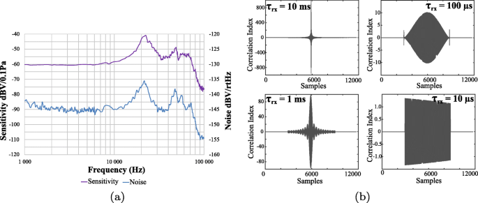
a SPU1410LR5H typical high frequency response and noise [26] b pulse compression of chirp with Δftx= 20 kHz, sample frequency of 196 kHz and constant pulse duration τtx=30 ms at different awake time durations (τrx)
-
2.
The audio broadcast duration (τtx), which should be as low as possible for an optimal compression ratio. However, limiting this parameter decreases the coverage range, as explained in Fig. 3.
-
3.
The receiver awake time (τrx). This parameter should be set with care. On the one hand, there is a direct relationship with the time-bandwidth. Increasing τrx improves the SNR and accuracy quadratically. On the other hand, the receiver awake time should be kept as low as possible to restrain the power consumption for a single measurement.

As a visual example, the pulse compression of a chirp with a nominal chirp bandwidth of Δftx=20 kHz and a constant pulse duration τtx=30 ms for different awake times are depicted Fig. 4b. Pulse compression is obtained by performing the cross correlation between the chirp extract and the entire linear chirp. Frequency domain cross correlation based on fast Fourier transformation is used with a complexity of
This complexity only depends on the transmitted signal since the chirp extract is zero padded to obtain two vectors of equal length, necessary in the used cross correlation algorithm. Figure 4b shows the influence of the chirp excerpt duration on the correlation index. The longer the recorded signal, the higher and narrower the latter. Correct maxima at a sufficient resolution can be derived from the pulse compression calculations when the awake time is limited to 1 ms.
3 Validation: simulation-based performance analysis
3.1 Simulation framework
We established a simulation framework to assess the performance of the proposed ranging system under realistic noise conditions and in reflective indoor environments. Specifically, the robustness of the inter-correlation performance in different positions, possibly suffering from reverberation, has been investigated. The simulation framework is based on the image source model (ISM), which has been extensively used in room acoustics because of its fast processing speed with accurate results in case of box shaped rooms [27]. The Allen and Berkley algorithm used in this ISM calculates the room impulse response (RIR) at the receiver’s position using a time-domain image expansion method, where wall reflections are replaced by virtual sources. All RIR calculations were performed in a 6 x 4 x 2.5 m room with rigid walls. The sound source is positioned slightly off the room center at a height of 1 m. This is done to prevent sweeping echoes [28] which occur in perfect cube shaped boxes due to the orderly time-alignment of high-order reflections. Both the sound source and the receiver positioned in this room are perfectly omnidirectional. The absorption coefficients of the walls are kept uniform over all 6 planes. This is accurate as long as the wavelength of the sound is small relative to the size of the reflectors [29]. The speed of sound is kept constant (340 m/s) considering a uniform room temperature of less then 20 ∘ C. The sample frequency is set to 196 kHz which is smaller than the common values offered by off the shelf microcontroller boards (nRF52832) and larger than the Nyquist frequency of the ultrasonic MEMS microphone maximum frequency (75 kHz). The audio broadcast duration τtx is fixed to 30 ms such that every possible sensor position in the simulation environment receives a sound signal during its wake-up period.
We performed two types of simulations in this acoustic shoe box. The first type is a Monte Carlo simulation to test the influence of signal bandwidth and additive colored noise on the accuracy of the pulse compression technique. During these simulations, the impact of the room characteristics, such as reflection, scattering, and reverberation, are kept as low as possible. The second type of shoe box simulations investigates the impact of the room’s characteristics by creating simulation environments with 600 distributed microphones.
3.2 Performance assessment
Monte Carlo simulations are performed to test the autocorrelation efficiency when noise is added to a chirp with different signal bandwidths. In a low-reverberant room, a single sensor receiver is positioned at a distance of 1.553 m from the source. The Monte Carlo simulation process is depicted in Fig. 5. The first two steps are conventional to the source image method: the room impulse response at the microphone is calculated and convoluted with the transmitted audio signal. In step 3, white noise is added to create sound signals with different SNR levels at the receiver. The next step consists of applying a 1 ms window to the noisy signal, mimicking the wake up time of the mobile nodes. In the final step of the simulation the emitted sound signal is correlated with the calculated, received sound signal, selecting the index of the correlation maximum and calculating the corresponding distance. The white noise addition, windowing and correlation processes are repeated for 10,000 times. Post-processing fits the acquired distances to a normal distribution and an Epanechnikov kernel distribution. The latter is chosen because of its optimal performance in a mean square error sense [30]. It shows a better smoothed kernel density estimate in the case of non-Gaussian distributions. Figure 6 illustrates the Gaussian and Epanechnikov distributions in the case of a 30 kHz bandwidth and an SNR of 6 dB. In the latter, we find secondary peaks offset by a single or multiple wavelengths from the calculated distance peak. In general, the Gaussian distribution provides a good measurement considering precision and accuracy.

Overview of the pre-processing, Monte Carlo simulations and post-processing. The actual Monte Carlo simulations are repeated 10 000 times

Normal and Epanechnikov distributions for a 30 kHz chirp with a SNR of 6 dB
Table 2 shows the accuracy (ε) and precision (σ) calculated from the Gaussian distribution of five different chirps at increasing signal to noise ratios. The lower frequency is fixed to 25 kHz; the upper frequency depends on the chosen chirp bandwidth, which is increased in steps of 10 kHz. As the attenuation of sound propagation is quasi linear with the frequency [31], we chose descending chirps, i.e., the further away from the sound source, the lower (and less attenuated) the signal within the wake-up window will be.
Two conclusions can be drawn from Table 2. The bandwidth dependency performs as expected, as increasing the bandwidth improves both accuracy and precision. The influence of additive white noise on the accuracy is minimal. Moreover, the lower chirp bandwidths are less sensitive to decreasing SNR, both regarding accuracy and precision. In noisy environments, a better performance is achieved by using these lower chirp bandwidth signals.
Measurements performed in a non-anechoic chamber show that the maximum frequency is limited to 45 kHz, although the datasheet of the SPU1410LR5H states that the microphone response can go as high as 75 kHz. The simulation results from above show that with a limited chirp bandwidth of 20 kHz (45 kHz down to 25 kHz), the accuracy and precision remain adequate to perform distance calculations.
3.3 Room characteristics simulations
We investigated the impact of the room characteristics, namely reflections, diffraction, and attenuation. Three shoe boxes are created, all with a different absorption coefficients: α=0.05, α=0.3, and α=0.9. These absorption coefficients are distinctively chosen and represent respectively an empty room with walls of standard brickwork, fiberboard, and acoustic plaster panels [32]. In these rooms, 600 microphones (20x30) are equally spread in one quadrant of the room, with a fixed distance of 10 cm between two sensors or a sensor and a wall. The microphones and the sound source are positioned in the same z-plane, at a height of 1 m. Table 3 shows the P50, P95, and mean distance errors of the pulse compression technique with a chirp bandwidth of 20 kHz in these three rooms with no noise added. The P50 value shows that half of the simulated distances have an error smaller than 3 cm in the most real world representative room (α2=0.3). The large difference between the mean and P50 value indicates that there are a lot of outliers. This is confirmed by the higher P95 values. To visualize the cause of these larger errors, a heatmap of the absolute value of the difference between the measured and the actual distance was generated (Fig. 7).

Heatmap of the distance simulation error in a room with absorption coefficients a α=0.05, b α=0.3, and c α=0.9. The absolute value of the autocorrelation in case of an ambiguous distance measurement (d) shows the difference between the correct peak (red line) and the maximum
It can be seen, as expected, that there is a considerable, negative effect of the reflections on the accuracy of the proposed system. The radius in which the ranging performs well decreases as the walls become more reflective. Inspection of the generated correlation data of an erroneous distance simulation, i.e., microphone 522 at a distance of 2.136 m in a room where α=0.05 (Fig. 7d), provides additional insights. The calculated distance corresponding with maximum correlation value is larger than the actual distance, indicated by the red line. Constructive interference of higher frequencies still present in the room can cause correlation peaks larger than the peak generated by the lower, effective distance frequency chirp.
4 Enhanced accuracy solutions
The previous section showed that utilizing the maximum correlation index as a selection criteria for the distance measurements results in an adequate solution, yet it does not yield the best distance estimate in many situations. In most cases, the correct maximum is the first one of a series of local maxima, as the lower frequencies are not present yet since the chirp signal descends. We propose three methods to select this first local peak and enhance the system’s accuracy: window functions, peak prominence, and delta peak approaches. The sole constraint of these methods is to keep the processing power as low as possible, as the energy consumption is proportional to it.
4.1 Method 1: Window functions
In the first method, window functions are applied to the correlation results, such that the first peaks of the local maxima are increased relatively to the others. The most straightforward window function is a linearly decreasing function. Figure 8 shows the cumulative density function (CDF) plots of the distance error for the original maximum method and when four different linear window functions are applied to the correlation data in the shoe box simulation environment with an absorption coefficient of (α=0.3). The absolute value of the negative slope of this function can not be larger than 1, as some correlation data would become negative and limit the maximum reachable distance. In general, applying a window function to the correlation results in an improved accuracy. The lowest P50, P95, and maximum distance error (P100) values are obtained with a slope of −1. We also investigated the potential improvement of applying a quadratic window function of the type y=±ax2+bx+c to check whether it is better to give more or less weight to the early peaks. We can deduce from the CDF plots in Fig. 8 that the positive quadratic function has an even better effect than the linear window function.

Cumulative density function of the ranging error when linear window functions with different slopes and positive and negative quadratic windows are applied to the correlation data
A faster initial decline consequently increases the influence of the earlier peaks, improving the accuracy. We tested with exponential window functions the limits of this fast, initial decline: y=ax−b in Fig. 9. A good measure of decay in exponential functions is the half-life time (T0.5). Smaller decay times (T0.5=1 ms) result in similar CDF plots as with a steep slope linear function. Choosing the half-life too large results in similar CDF plots as the positive quadratic function. The optimal exponential function is the one with a decay time of T0.5=3 ms, a tenth of the original broadcasted signal. When comparing the optimal exponential window function to the quadratic function, it is clear that the P95 value of this window performs better but the maximum distance errors are larger. A choice between a more precise or more accurate system can be made here.

Cumulative density function of the ranging error when exponential window functions with different bases are applied to the correlation data
4.2 Method 2: Peak prominence
The major discrepancy of the window function method occurs due to the significance it gives to the earlier correlation data. It works well for microphones close to the speaker but as the difference between the maxima decreases with larger distances, peaks earlier than the correct maximum are chosen, resulting in even larger errors. We further improved the accuracy by searching the local maxima without modifying the pulse compression data. The prominence of a peak indicates how much the peak stands out because of its intrinsic height and its location relative to other peaks [33]. It can be calculated as follows: extend a horizontal line from a chosen peak to the left and the right until the line crosses a signal because either there is a higher peak, or it reaches the left or right end of the signal. Find the minimum of the left and right interval (min 1 and min 2 in Fig. 10). This point can be a valley or a signal endpoint. Calculate the prominence by taking the difference between the height of the peak and the higher minimum of the two intervals. A low, isolated peak can be more prominent than a higher member of a tall range (Fig. 10). This technique is commonly used in topography, in which it represents the elevation of a mountain summit relative to the surrounding terrain, and serves as a criterion to define a separate peak [34, 35]. The index used for distance calculations is selected by calculating the prominence of all correlation peaks, setting a prominence threshold, the peak prominence factor (PPF), and using the index of the first peak in the array of the prominences larger than the threshold. Both reflections and noise affect the prominence of signals. The influence of the reflections on the accuracy is minimal as, in a line-of-sight scenario, the correlated maxima of these reflections are positioned later then the original sound signal. Noise on the other hand can reduce the prominence of the correlated peaks, lowering the distinctness of the local maxima, and complicate the PPF determination.

Peak prominence method compared to the maximum method. The correct distance peak is the first of a series of local maxima and correctly appointed to by the peak prominence method
The simulations show a clear exponential relationship between the SNR and the optimal PPF (Fig. 11). Determining the SNR requires additional measurements or noise power estimation techniques, both requiring extra energy on processing and power level. Setting a fixed prominence factor can resolve this problem. However, choosing the PPF too low includes erroneous noise peaks to the array, while choosing it too high excludes the real distance peaks, resulting in a similar effect as the maximum method. Figure 12 depicts the mean, P50, and P95 values of the distance error at different PPFs in the case of a 20 dB signal to noise ratio. In case of the P95 values, a passband of adequate PPF’s can be derived (purple line, here with an upper and lower cut-off value 0.25 m above the minimum P95 value). These error bands are plotted as bars in Fig. 11 and are proportional to the SNR. A single value (PPF = 65) can be derived from this figure in which the peak prominence method operates adequately for the different SNR values.

Optimal PPF based on the P95 values for simulations with different white noise SNRs. The cutoff for the distance errors is set to 25 cm (error bars). An exponential curve can be fit for optimal PPF selection

Mean, P50, and P95 values of the distance error for different PPF values in a simulation where the white noise SNR is set to 20 dB
4.3 Method 3: Delta peak
We explore the delta peak method as an alternative to improve the system’s accuracy. In this approach, the difference between two consecutive local maxima is calculated and the peak following the largest positive difference is selected for further distance estimations. This method computationally less complex than the peak prominence method and also does not alter the correlated data. However, the complexity reduction impairs the accuracy. This can be seen on the CDF of the original and adapted methods for a room with α=0.3 and a SNR of 3 dB, charted in Fig. 13. For example, 63% of the delta peak distance calculation errors is smaller than 10 cm, in comparison to 56% with the maximum method, 68% with the quadratic window method, and 73% with the peak prominence method. Additionally, the robustness against reflective room characteristics is the lowest of all techniques. As for the maximum method, the large delta values imply the wrong index due to positive interference, lowering the system’s accuracy. The delta peak heatmap in Fig. 14 shows these outliers close to the corners and walls of the simulated environment.

Cumulative density functions of the distance error of the proposed optimization methods in a room with α=0.3 and SNR = 3 dB

Heatmaps of the distance error of the different enhanced accuracy solutions in a simulation environment with absorption coefficient α=0.3 and the SNR = 3 dB. With a the maximum, b the positive quadratic filter, c peak prominence, and (d) delta peak method
Figure 15 represents the mean and median (P50) distance error of all proposed methods when different levels of white noise are added. The peak prominence approach has the highest accuracy, even at a very low SNR. Fixing the local peak threshold resolves in a similar, negative SNR-dependency as the other methods. Of the two remaining methods, the positive quadratic window function performs best. The difference between the mean and median values indicates that there are high outliers.

SNR influence on the mean and median (P50) distance error (m) of the four proposed methods
5 Experimental validation: results and discussion
We have built a low-power setup to test the proposed system design, the pulse compression technique, and methods to improve the accuracy in a real-life environment. The set-up focuses on the key acoustic components of the system described in Section 2.2. The acoustic transmitter and receiver are realized in hardware and the RF-based wake-up is implemented through a cable link between the two entities for proof of concept validation.
5.1 Experimental setup and hardware prototype
Figure 16 depicts the system in an empty 6 x 4.27 x 3.41 m room in which the walls consist of plaster wood and glass, the floor of ceramic tiles, and the ceiling of rock wool on solid backing. Three RT60 measurements were performed to test the reverberation time of this room. The average value and uncertainty at the different frequencies can be found in Table 4Footnote 2.

Picture of the setup in measurement environment and schematic representation of the simplified system design
Power measurements of the LDO, MEMS, and OPAMPS are performed with a 4 points measurement on a Hameg HM8112-3 precision multimeter
To receive the ultrasonic sound signals at low-power, dedicated hardware has been designed based on an ultra low-power acoustic array [36]. Ultrasonic MEMS microphones (SPU1410LR5H [26]) are used as sound transducers (Fig. 17). The advantages of these MEMS microphones over ultrasonic piezo elements are their omnidirectional response, small form factor, and high bandwidth. The two opamps (TLV341 [37]) have a large gain bandwidth product, to boost the low amplitude signals coming from the microphone. The acoustic measurements on the MEMS and amplification circuit show a maximum detectable frequency of 45 khz. Active filters are added to the cascading opamps to narrow the amplified signals to the limited bandwidth in the ultrasonic domain (25 to 45 khz). A fixed LDO voltage regulator is added as a supply for the MEMS microphone and as an input offset voltage to guarantee a rail-to-rail output. The output of this ultrasonic receiver is then sampled and used as an input signal for the pulse compression. The acoustic data was sampled with a NI-USB-6212 DAQ [38] in our experiments. The sample frequency and data resolution are adapted to mimic the ADC used in common microcontrollers, (196 kS/s and 12 bit). Further processing of the collected data is done in a Matlab environment.

Polar plot of the measured, relative, XY directionality of the Fostex FT17H tweeter @25 kHz in non-anechoic chamber
The components above are specifically chosen to fulfill the low-power requirements. The LDO and amplifiers are equipped with power down pins, reducing the quiescent power consumption when the ranging system is not activated. Table 5 summarizes the power usage of these components and the estimated power usage of a nRF52832’s ADC, as described in the datasheet. Because of the short awake time of the mobile node, the power consumption in passive state has a major contribution to the total power consumption. This system could operate on a standard single coin cell battery (CR2032: 3 V, 225 mAh [39]) for more than 8.5 years if the receiver would wake up once every second. This equals the battery shelf life. Note that wake-up times of the LDO, microphone, ADC, or opamps can increase the power consumption significantly.
The transmit side consists of the following elements: a DAC, a commercially available amplifier circuit, and an ultrasonic speaker. Here, the NI-USB-6212 DAQ is used as a DAC to generate two signals: the 45 to 25 kHz chirp and the “start-sampling” signal. The latter signal is sent over the cable to the receiver side and consists of a pulse at TA imitating the RF wake-up. This pulse initiates a 1ms sampling time at the receiver DAQ. The DAC chirp signal is amplified with a commercially available amplifier circuit, based on a TDA7492 class-D opamp. In-house tests have show that it has an amplification bandwidth over the intended 45 khz. As an ultrasonic sound speaker, the Fostex FT17H is chosen. Its ultrasonic capabilities comes at a cost, limiting the directionality on a XY-plane to 30 ∘ at a 25 kHz sine wave (Fig. 17).
5.2 Ranging measurements
We evaluated the accuracy of the proposed solution by performing acoustic measurements in a quadrant of the room, in which 63 measurement points with a mutual distance of 30 cm were dispersed. Three types of scenarios were tested: with the speaker directed to the x- or y-axis, with the speaker directed to the microphone and with an adapted, quasi-omnidirectional speaker. As in the simulations, the sound source is located at an off-centered position.
The first measurement scenario shows that the signal power received outside the directional speaker’s beam is limited, resulting in large accuracy errors, as can be seen in Fig. 18a, b. To obtain a quasi-omnidirectional speaker, a semi-sphere is put on a distance from an upwards oriented tweeter, reflecting the sound in all possible directions. Tests in the audible domain show only a difference of 6 dB between the maximum and minimum measured sound intensity level caused by the structure of the speaker. This method addresses the preeminent scenario in which the directional sound source is directed towards the receiver, and only reflections from the walls in the speaker direction are received by the microphone (Fig. 18c).

Heatmap of the maximum method in different measurement scenarios: when the speaker is aimed towards the x-axis (a), towards the y-axis (b), towards each microphone position individually (c), and towards the z-axis with a semi-sphere (quasi-omnidirectional speaker) (d)
The results of the maximum method applied on these quasi-omnidirectional speaker measurements are in line with the corresponding simulations (Fig. 18d). The accuracy of these measurements is high for microphones close to the sound source. If the distance is increased or the microphone is closer to a wall, the accuracy drops. Figure 19 shows that the median of the distance error in this scenario is 0.108 m. The large P95 value (1.608 m) reveals again a number of outliers.

CDF plot of the improved accuracy methods on quasi-omnidirectional measurements with a a lower and b a higher SPL
We applied the aforementioned improved accuracy methods to two sets of measurement data, representing a low and high SNR scenario. The CDF plots of these two measurements can be found in Fig. 19. In the higher SPL scenario, all of the proposed methods show the behavior that is anticipated by the simulations except one: the delta peak method. The smaller amount of outliers in this method results in a lower P100 value than the maximum method, and we can conclude that in the higher SPL measurements, all of the proposed methods have a higher accuracy than the original maximum method. The P50 and P95 values are lower than 10 cm and 50 cm respectively.
We noticed a risk when the received sound signal power is reduced. At higher P values (> P80), the curves do not follow the same path as in the simulation and higher SPL scenarios. In these measurements, the peak prominence and maximum method have the best P100 (1.984 m) values. The smaller mean and P95 value of the peak prominence method confirm that this method has a lower amount of larger errors making this method more robust than the maximum method. The delta peak in the measurements method shows a similar behavior as in the simulations where the large distance error outliers lead to a method that performs worse than the original maximum method. Comparable results are found for the positive quadratic window method. A more detailed CDF plot of the applied window methods (Fig. 20) shows that the two optimal window functions, the exponential window with a half life of 3 ms and the positive quadratic function, perform worse than the data without any window, in contrast to the results from simulations. The linear function performs best. When comparing the correlation data of the window functions on a single position with low accuracy, it is clear that the early correlation peaks in the case of the positive quadratic and exponential windows are overamplified and larger than the actual distance peak. This increases the distance error.

Cumulative density function of the proposed window functions on the measurement data performed with the quasi-omnidirectional speaker
6 Conclusions and future work
We have presented and demonstrated a novel hybrid signaling distance measuring system. The system is able to perform cm-accurate distance measurements with sampled and short (196 sampled during 1ms) ultrasonic chirp signals on a restricted energy budget. Monte Carlo and acoustic shoe box simulations with 600 distributed microphones show centimeter accuracy close to the sound source for the synchronized wake-up and pulse compression method. This accuracy is in line with the current state-of-the-art indoor positioning systems, often performed in artificial environments [40]. We proposed three lightweight and fast methods to improve the accuracy near reflective objects with a limited processing power. The peak prominence method improves the accuracy in the low SNR scenario’s with a factor 10 for the P95 values. Experimental verification with an in-house developed ultrasonic receiver validates the enhanced accuracy methods and confirms the low-power acoustic reception and processing, with a power consumption of 2.074 μW for a single 1 ms measurement or over 8.5 years of operation on a CR2032 coin cell battery. This power consumption is 3 orders of magnitudes more efficient than BLE-indoor positioning technique proposed by [41]. Our results are in agreement with previous analyses [19, 42] demonstrating comparable results with the used autocorrelation method. In our future work, we will extend the experimental set-up with the RF signaling.
Next, a calibration solution will be worked out to determine the start-up time of the receiver hardware components, as it may impact both precision and power consumption.
The presented ranging method can be extended to perform positioning. Extra sound sources should be added to the set-up for positioning purposes in a 2D and 3D environment. Consequently, at the awake time, three signals may be received at the same time. Needless to say, identifying which signal comes from which source is the main concern here. A more detailed investigation should reveal which multiple access protocol is suited to address this challenge and existing chirp based techniques [21–23] should be tested. The robustness against Doppler shifts of the acoustic chirps [43] needs to be verified and tracking algorithms to counter the potentially introduced error can be investigated.
Availability of data and materials
The datasets generated and/or analyzed during the current study are available in the High-Precision-Hybrid-RF-and-Ultrasonic-Chirp-based-Indoor-Ranging-for-Low-Power-IoT-Nodes repository, DOI: 10.5281/zenodo.3269747
Notes
This is an area around a beacon, in which mobile nodes can measure their distance to that beacon.
The given RT60 values are measured specifically in the audible domain. The RT60 values in the ultrasonic domain will be lower, as the reverberation time is inversely proportional to the frequency.
Power measurements of the LDO, MEMS, and OPAMPS are performed with a 4 points measurement on a Hameg HM8112-3 precision multimeter
Abbreviations
- ADC:
-
Analog-to-digital converter
- CDF:
-
Cumulative density function
- CDMA:
-
Code-division multiple access
- DAC:
-
Digital-to-analog converter
- DAQ:
-
Data acquisition system
- FDMA:
-
Frequency-division multiple access
- ISM:
-
Image source model
- LDO:
-
Low dropout
- MEMS:
-
Microelectromechanical systems
- PPF:
-
Peak prominence factor
- RF:
-
Radio frequency
- RIR:
-
Room impulse response
- RT60:
-
Reverberation time 60 dB
- SNR:
-
Signal to noise ratio
- SPL:
-
Sound pressure level
- TDMA:
-
Time-division multiple access
- TDoA:
-
Time difference of arrival
- ToA:
-
Time of arrival
References
H. Kuttruff, Room Acoustics, vol. 6 (Taylor and Francis Group, Boca Raton, 2017).
S. Li, R. Rashidzadeh, in 2018 IEEE International Conference on Electro/Information Technology (EIT). A hybrid indoor location positioning system, (2018), pp. 0187–0191. https://doi.org/10.1109/eit.2018.8500265.
Q Lin, Z An, L Yang, Rebooting ultrasonic positioning systems for ultrasound-incapable smart devices. MobiCom ’19, 1–16 (2019).
M. Addlesee, R. Curwen, S. Hodges, J. Newman, P. Steggles, A. Ward, A. Hopper, Implementing a sentient computing system. Computer. 34(8), 50–56 (2001).
N. B. Priyantha, The cricket indoor location system. PhD thesis, Computer Science and Engineering, MIT (2005).
C. Medina, C. J. Segura, A. De la Torre, Ultrasound indoor positioning system based on a low-power wireless sensor network providing sub-centimeter accuracy. Sensors. 13:, 3501–3526 (2013).
O Khyam, J Alam, A. J. Lambert, A. M. Garratt, M. R. Pickering, Highprecision OFDM-based multiple ultrasonic transducer positioning using a robust optimization approach. Sensors. 16(13), 5325 (2016).
Y. Zhao, J. R. Smith, A battery-free RFID-based indoor acoustic localization platform. IEEE Int Conf RFID, 110–117 (2013). https://doi.org/10.1109/rfid.2013.6548143.
B. Cox, L. De Srycker, L. Van der Perre, Acoustic backscatter: Enabling ultralow power,precise indoor positioning, UPINLBS ’18, (2018).
X. Li, L. Xu, C. Cai, L. Xu, A. Salo, in 2008 IEEE International Conference on Mechatronics and Automation. Estimation of power consumption of miniature audio directional transducer (Takamatsu, 2008), pp. 95–98.
J. Kolakowski, V. Djaja-Josko, M. Kolakowski, K. Broczek, UWB/BLE tracking system for elderly people monitoring. Sensors. 20(6), 1574 (2020).
PUI Audio, Low-noise bottom port piezoelectric MEMS microphone with wake on sound feature. Rev. B, 1–7 (2017).
D. H. Goldberg, A. G. Andreou, P. Julian, P. O. Pouliquen, L. Riddle, R. Rosasco, Awake-up detector for an acoustic surveillance sensor network: Algorithm and VLSI implementation, ISPN ’04, (2004).
D. Munoz, F. L. Bouchereau, C. Vargas, R. Enriquez-Caldera, Position location techniques and applications, 1st edn (Academic Press, Elsevier, Burlington, 2009).
X. Chen, Y. Chen, S. Cao, L. Zhang, X. Zhang, X. Chen, Acoustic indoor localization system integrating TDMA+FDMA transmission scheme and positioning correction technique. Sensors. 19(10), 2353 (2019).
A. Tadayon, M. Stojanovic, Iterative sparse channel estimation and spatial correlation learning for multichannel acoustic OFDM systems. IEEE Journal of Oceanic Engineering. 44(4), 820 (2019).
F. Yuan, Z. Jia, E. Cheng, Chirp-rate quasi-orthogonality based DSSSCDMA system for underwater acoustic channel. Applied Acoustics. 161:, 107163 (2020).
M. Parrilla, A. J., C. Fritsch, Digital signal processing techniques for high accuracy ultrasonic range measurements. IEEE Trans. Instrum. Meas.40(4), 759–763 (1991).
K. Nakahira, T. Kodama, S. Morita, S. Okuma, Distance measurements by an ultrasonic system based on a digital polarity correlator. IEEE Trans. Instrum. Meas.50(6), 1748–1752 (2001).
A. Hammoud, M. Deriaz, D. Konstantas, Robust ultrasound-based roomlevel localization system using COTS components, UPINLBS ’16, (2016).
S. Murano, C. Pérez-Rubio, D. Gualda, F. J. Álvarez, T. Aguilera, C. D. Marziani, Evaluation of Zadoff–Chu, Kasami, and chirp-based encoding schemes for acoustic local positioning systems. IEEE Trans. Instrum. Meas.69(8), 5356–5368 (2020).
Y. Bai, P. J. Bouvet, Orthogonal chirp division multiplexing for underwater acoustic communication. Sensors. 18(11), 1 (2018).
M. O. Khyam, S. Sam Ge, X. Li, M. Pickering, Orthogonal chirpbased ultrasonic positioning. Sensors. 17: (2017).
P. Lazik, A. Rowe, in Proceedings of the 10th ACM Conference on Embedded Network Sensor Systems. Indoor pseudo-ranging of mobile devices using ultrasonic chirps, (2012), pp. 99–112.
A. Hein, Processing of SAR data: fundamentals, signal processing, interferometry (Springer, 2004). https://doi.org/10.1111/j.0031-868x.2004.295_5.x.
Knowles Acoustics, SPU1410LR5H-QB: zero height ultra-mini SiSonicTM microphone specification with MaxRF protection and extended low frequency performance. Rev. A, 1–12 (2013).
J. Allen, D. Berkley, Image method for efficiently simulating small-room acoustics. J. Acoust. Soc. Am.65:, 943–950 (1979).
E. De Sena, N. Antonello, M. Moonen, T. van Waterschoot, On the modeling of rectangular geometries in room acoustic simulations. IEEE/ACM Trans. Audio Speech Lang. Process. 23(4), 774–786 (2015).
R. Scheibler, E. Bezzam, I. Dokmanić, Pyroomacoustics: a python package for audio room simulations and array processing algorithms. Comput. Sci. Sound (2017). http://arxiv.org/abs/http://arxiv.org/abs/1710.04196v1.
V. A. Epanechnikov, Non-parametric estimation of a multivariate probability density. Theory Probab.Appl.14(1), 153–158 (1967).
M. Vorländer, Auralization: fundamentals of acoustics, modelling, simulation, algorithms and acoustic virtual reality, vol. 1 (Springer, Berlin Heidelberg, 2008). An optional note.
Akustik, Absorption coefficients. http://www.acoustic.ua/st/web_absorption_data_eng.pdf. Accessed 12 Feb 2019.
O. Z. Chaudhry, W. A. Mackaness, Creating mountains out of mole hills: automatic identification of hills and ranges using morphometric analysis. Trans. GIS. 12(5), 567–589 (2008).
F. Press, R. Siever, Earth, 3rd edn. (W H Freeman and Company, San Francisco, 1982).
M. A. Summerfield, Global geomorphology (Longman, London, 1991).
B. Thoen, G. Ottoy, L. De Strycker, An ultra-low-power omnidirectional MEMS microphone array for wireless acoustic sensors. Sensors (2017). https://doi.org/10.1109/icsens.2017.8234392.
Texas Instruments, TLV34XX: low-voltage rail-to-rail output CMOS operational amplifiers with shutdown. Rev. D, 1–39 (2016).
National Instruments, USB-6212: 16 AI (16-Bit, 400 kS/s), 2 AO (250 kS/s), Up to 32 DIO USB Multifunction I/O Device. Rev., 1–14 (2017).
Panasonic, CR2032: manganese dioxide lithium coin batteries. Rev. A, 1–6 (2005).
F. Zafari, A. Gkelias, L. K. K., A survey of indoor localization systems and technologies. IEEE Commun. Surv. Tutorials. 21(3), 2568–2599 (2019).
S. Sadowski, P. Spachos, RSSI-based indoor localization with the Internet of Things. IEEE Access. 6:, 30149–30161 (2018).
D. Marioli, N. C., C. Offelli, D. Petri, E. Sardini, A. Taroni, Digital time-of-flight measurement for ultrasonic sensors. IEEE Trans. Instrum. Meas.41(1), 93–97 (1992).
T. Aguilera, F. J. Álvarez, J. A. Paredes, J. A. Moreno, Doppler compensation algorithm for chirp-based acoustic local positioning systems. Digit. Signal Process.100:, 102704 (2020).
Acknowledgements
We would like to thank BlooLoc for the low-power challenge on which this idea sprouted. We are also grateful to Gilles Callebaut for his reviewing and editing work.
Funding
This work has been partly funded by the Flemish governmental Agency for Innovation and Entrepreneurship (VLAIO) in the frame of the project YOUBEEPLUS (HBC.2017.0413).
Author information
Authors and Affiliations
Contributions
BC contributed in conceptualization, software and hardware development, investigation, methodology, simulations, result analysis, draft manuscript writing, manuscript reviewing, and editing. LVDP, GO, SW, and LS contributed in the conceptualization, validation, draft manuscript reviewing, and editing. The authors read and approved the final manuscript.
Corresponding author
Ethics declarations
Competing interests
The authors declare that they have no competing interests.
Additional information
Publisher’s Note
Springer Nature remains neutral with regard to jurisdictional claims in published maps and institutional affiliations.
Rights and permissions
Open Access This article is licensed under a Creative Commons Attribution 4.0 International License, which permits use, sharing, adaptation, distribution and reproduction in any medium or format, as long as you give appropriate credit to the original author(s) and the source, provide a link to the Creative Commons licence, and indicate if changes were made. The images or other third party material in this article are included in the article’s Creative Commons licence, unless indicated otherwise in a credit line to the material. If material is not included in the article’s Creative Commons licence and your intended use is not permitted by statutory regulation or exceeds the permitted use, you will need to obtain permission directly from the copyright holder. To view a copy of this licence, visit http://creativecommons.org/licenses/by/4.0/.
About this article

Cite this article
Cox, B., Van der Perre, L., Wielandt, S. et al. High precision hybrid RF and ultrasonic chirp-based ranging for low-power IoT nodes. J Wireless Com Network 2020, 187 (2020). https://doi.org/10.1186/s13638-020-01795-1
Received:
Accepted:
Published:
DOI: https://doi.org/10.1186/s13638-020-01795-1